Simulative Comparative Analysis of Blind Source Separation Algorithms

(1)

ISSN (Print) : 2320 – 3765 ISSN (Online): 2278 – 8875

I

nternational

J

ournal of

A

dvanced

R

esearch in

E

lectrical,

E

lectronics and

I

nstrumentation

E

ngineering

(An ISO 3297: 2007 Certified Organization)

Vol. 5, Issue 6, June 2016

Simulative Comparative Analysis of Blind

Source Separation Algorithms

Aditi Singla , Jyoti Saxena

M.Tech Student, Department of ECE, GZSCCET, Bathinda, Punjab, India

Professor, Department of ECE, GZSCCET, Bathinda, Punjab, India

ABSTRACT: Independent vector analysis, a powerful blind source separation technique, is an extension from uni-variate components to multiuni-variate components. In this paper, over determined case of instantaneous noisy mixtures is considered for separation in frequency domain. The source separation is done by two algorithms and their performance has been compared. The performance of natural gradient algorithm is compared with new independent vector analysis blind source separation algorithm. It is observed that new independent vector analysis blind source separation algorithm exhibited lesser mean square error than natural gradient algorithm.

KEYWORDS—Blind source separation, Natural gradient, Independent vector analysis, convergence speed, step size.

I. INTRODUCTION

In blind source separation (BSS), multiple independent source signals are extracted from their mixtures with little or no knowledge about the sources and the mixing system. Numerous applications of BSS have been found in a wide variety of fields, such as antenna arrays for wireless communications, biomedical signal processing, seismic signal processing, passive sonar, and speech processing [1,2]. It has been shown that the natural gradient improves dramatically the learning efficiency in blind separation [3]. For the standard case where the number of sources is equal to the number of sensors, the natural gradient algorithm has been developed by Amari et al. [4] and independently as the relative gradient by Cardoso [5]. However in most practical cases, the number of active source signals is unknown and changing over time. Therefore in the general case the mixing matrix and demixing matrix are not square and not invertible. Source separation has been done when number of sources equal to or greater than the number of sensors [6, 7]. It is plausible to use over-determined mixtures, where the number of sensors is not less than the number of sources, to improve upon blind source separation algorithms in extracting the signals of interest from mixtures. The natural gradient algorithm is used to derive an efficient learning algorithm and to minimize the effect of noise on the output signals [8].

In this paper, we examine blind separation of over-determined mixtures. First, performance of separated signals using natural gradient is computed. Then this performance is compared with new IVA BSS algorithm [9, 10].This paper is organized as follows: Section 2 describes the Blind source separation of over-determined mixture. Section 3 demonstrates and describes simulations and experimental results. Finally, some conclusions are drawn in section 4.

II. BLIND SOURCE SEPARATION OF OVERDETERMINED MIXTURE

Blind source separation deals with recovery of source signals from a mixture without knowing the mixing system. The term blind indicates that there is no a priori knowledge about the source signals. Assume that the unknown source signals s(t) = (s (t), … … s (t)) are zero-mean processes and mutually statistically independent and x(t) = (x (t), … … x (t)) is an available sensor vector, which is a linear instantaneous mixture of sources represented in equation (1)

(2)

I

nternational

J

ournal of

A

dvanced

R

esearch in

E

lectrical,

E

lectronics and

I

nstrumentation

E

ngineering

source signals and the mixing matrix A except for independence of the source signals. The demixing model is a linear transformation in the form as represented in equation (2)

y(t) = Wx(t) (2) where y(t) = (y (t), … … y (t)) is an estimate of source signals s(t) and W is a demixing matrix.

a)Natural gradient blind source separation algorithm

For demonstration purposes, sources are randomly mixed and noise is added resulting in a mixture which is noisy and random in nature. Now, to estimate signals from the received mixture, natural gradient is applied. Block diagram of natural gradient IVA BSS is shown in Fig.1.Following are the steps followed:

( )

( ) … . … .

( )

( ) … …

( )

Fig.1: Block diagram of Natural gradient IVA BSS

i. Short time Fourier transform

It is Fourier related transform used to determine frequency and phase content of local sections of time varying signal. It is defined as in equation (3)

x(τ,ω) =∫ x(t)d(t− τ)e dt (3) where d (t) is window function and ω is angular frequency and τ isdummyvariable.Window can be hanning, hamming, Kaiser, Nuttal, blackman and Harris. These can be periodic or symmetric. Window length can be of length 512, 1024, 2048 or 4096.But hanning window (type periodic) of length 512 gives good convergence speed because of reduction in multiplication complexity. Multiplication complexity is given by log .

ii. Centering

It is applied to center the observation vector x by subtracting its mean vector. This implies that signal s is zero mean and the mixing matrix A remains the same after centering process.

iii. Whitening

(3)

I

nternational

J

ournal of

A

dvanced

R

esearch in

E

lectrical,

E

lectronics and

I

nstrumentation

E

ngineering

iv. Natural gradient

This criterion has the basic form of minimizing a cost function F(W)with respect to the demixing parameter W. There are also constraints that restrict the set of possible solutions. A typical constraint is to require that the solution vector must have a bounded norm, or the solution matrix has ortho-normal columns.

For the unconstrained problem of minimizing a multivariate function, the most classic approach is steepest descent or gradient descent. In gradient descent, we minimize a function F(W) iteratively by starting from some initial pointw(0), computing the gradient of F(W) at this point, and then moving in the direction of the negative gradient or the steepest descent by a suitable distance. Once there, we repeat the same procedure at the new point, and so on. For

= 1,2 … …we have the update rule as in equation (4)

w(t) = w(t−1)−∝(t) ( ) | ( ) (4)

with the gradient taken at the point ( −1).The parameter ∝(t) gives the length of the step in the negative gradient direction which is a positive scalar coefficient. It is often called the step size or learning rate. Iterations are continued until the natural gradient algorithm converges, which in practice happens when the Euclidean distance between two consequent solutions ||w(t)−w(t−1)|| goes below some small tolerance level. Rewriting the Euclidean distance as in equation (5)

w(t)−w(t−1) =Δw (5) Rewriting the equation (4) as in equation (6)

Δw =−∝ ( ) (6) Using the proportionality sign in above equation, it can be written as in equation (7)

Δw⋉ ( ) (7) The vector on the left hand side,Δw, in equation (7) has the same directionas the gradient vector on the right hand side, but there is a positive scalar coefficient by which the length can be adjusted.

The choice of an appropriate step length or learning rate ∝(t) is essential. Too small a value will lead to slow convergence and too large a value will lead to overshooting and instability, which prevents convergence altogether. Therefore determining a good value for the learning rate is essential.

b) New Independent Vector Analysis Blind Source Separation Algorithm

It is a technique for performing separation of multiple datasets. Multiple datasets can be represented as in equation (8):

R(t) = M∗s(t) + N (8) where R(t)noisy mixed signal or noisy mixture, M is unknown mixing matrix,s(t) is a set of statistically independent signals and N is assumed to be stationary, spatially and temporally white. Block diagram of new IVA BSS is shown in Fig.2. Again, for estimation of sources from over-determined mixture, new IVA BSS method is applied. Its steps are- centering and whitening, joint Diagonalization and source separation. Centering and whitening have been discussed in section II a (ii, iii). Joint Diagonalization is explained as follows:

(i) Joint Diagonalization

The new IVA BSS technique utilizes the ‘useful’ information in local regions of time-frequency plane, leaving behind the information in the entire time domain. Spatial time frequency distribution (STFD) matrices derived based on the short time Fourier transform (STFT) are represented in equation (9)

U (t, f) =∫ R(w)d(t−w)e dw (9) where d(t)is a window function. Further, auto and cross terms of STFD matricesP , (t, f) are defined as represented

in equation (10)

P , (t, f) =∬s (w)s∗ (w )d(t−w)d(t− w )e dwdw (10)

where * denotes the conjugate transpose of a vector. Due to overlapping of local frequency contents,P , (t, f) may be

(4)

I

nternational

J

ournal of

A

dvanced

R

esearch in

E

lectrical,

E

lectronics and

I

nstrumentation

E

ngineering

maxima of the gradient function and P , (t, f) becomes diagonal at these positions. At the selected time-frequency

points that is ‘single auto terms positions’, unitary matrix V is estimated by joint diagonalizing different whitened STFD matrices at the time frequency point. Then sources are estimated by using equation (11)

Estimatedsources = V∗ whiteneddata (11)

( )

( ) … . … .

( )

( ) … . .

( )

Fig.2: Block diagram of new IVA BSS

III. SIMUSLATIONS AND EXPERIMENTAL RESULTS

Blind source separation method is implemented on mixture of statistically independent signals to separate them. The source signals are taken of length 256. Then, these source signals are mixed through mixing matrix and noise is added. Simulations are done using

1. Natural gradient algorithm

2. New independent vector analysis blind source separation

Natural gradient algorithm is implemented for separating sources from mixed signal. For calculation of convergence speed of natural gradient algorithm, learning rate is varied from the 0.001 to 0.99 because convergence speed depends upon learning rate. Then by keeping the number of sources fixed that is three and by varying the number of observations, their effect is studied with respect to mean square error. Similarly, by varying SNR, again effect is studied with respect to MSE for different number of observations.

1. Number of sources is three and number of observations is four

(5)

I

nternational

J

ournal of

A

dvanced

R

esearch in

E

lectrical,

E

lectronics and

I

nstrumentation

E

ngineering

Fig.3: Three original source signals

After random mixing and addition of Gaussian noise, received mixture is random and noisy. Then using natural gradient algorithm, sources are estimated as shown in Fig.4.

Fig. 4: Estimated source signals

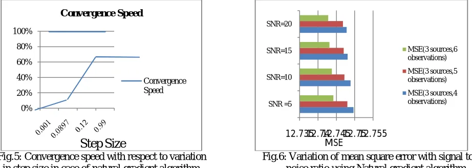
For calculation of convergence speed of natural gradient algorithm, it provides good convergence speed at learning rate of 0.12.Fig.5 shows the effect of change in step size on convergence speed.

Fig.5: Convergence speed with respect to variation Fig.6: Variation of mean square error with signal to in step size in case of natural gradient algorithm noise ratio using Natural gradient algorithm

Now, for computing the performance of estimated signals from the noisy and random mixture, performance parametric mean square error is calculated. Then by varying SNR from 5-20 at the difference of five, MSE is computed in Fig. 6.It can be seen that a significant decrease in MSE with increase in SNR.

2. Another experiment is conducted to evaluate the performance of source separation using new independent vector analysis method. For calculation of convergence speed of new independent vector analysis method, threshold value is varied. Then by keeping the number of sources fixed and by varying the number of observations; their effect is studied with respect to mean square error. Similarly, by varying SNR, effect is studied with respect to MSE.Fig.7 shows original signal. Fig.8 represents the recovered signals using new IVA BSS.

Fig.7: Original three signals Fig.8: Recovered signals

0% 20% 40% 60% 80% 100%

Convergence Speed

Convergence Speed

Step Size

12.73512.7412.74512.7512.755

SNR =5 SNR=10 SNR=15 SNR=20

MSE(3 sources,6 observations)

(6)

I

nternational

J

ournal of

A

dvanced

R

esearch in

E

lectrical,

E

lectronics and

I

nstrumentation

E

ngineering

For examining the convergence speed of new IVA method, threshold value is varied from 1.2∗10^−8 to 1.5∗10^−

8.It is found that the threshold value of 1.4∗10^−8 gives good convergence speed. Then effect of change in threshold value on convergence speed is shown in Fig.9. Fig.10 shows the variation of MSE with respect to SNR by varying number of observations.Again,it is seen that MSE decreases significantly with increase in SNR.

Fig.9: Converegnce speed with respect to variation Fig.10: Variation of mean square error with signal of threshold value in new IVA BSS algorithm to noise ratio using new IVA BSS

IV. CONCLUSION

New independent vector analysis blind source separation tackles the problem of separating signals from noisy mixtures.Results indicate the robustness of the new independent vector analysis blind source separation as compared to natural gradient algorithm in terms of MSE.As with increase in SNR, MSE for both these methods decreases.Also with increase in number of observations for separting signals from the mixture, MSE decreases indicating the improved separation performance of sources.

REFERENCES

[1] Aapo Hyvarinen, Juha Karhunen and Erkki Oja, “Independent Component Analysis, “A willey interscience publication, pp.1-503, 2001. [2]J. Escudero, “Applications of Blind Source Separation to the Magneto encephalogram Background Activity in Alzheimer’s Disease,” Thesis

doctoral file at university of Valladolid, pp.1-410, 2010.

[3] S.Amari, “Natural gradient works efficiently in learning,” Neural Computation, pp.251-276, 1998.

[4] S. Amari,A.Cichocki and H.H. Yang, “ A new learning algorithm for blind signal separation,” Advances in Neural Information Processing,pp.757-763,1996.

[5] J.F. Cardoso and B. Laheld, “Equivariant adaptive source separation,” IEEE Trans. SignalProcessing, pp.3017-3030, 1996.

[6] T.W. Lee, M.S.Lewicki and M. Girolami, “Blind source separation of more sources than mixtures using over-complete representations,”IEEE Signal Processing Letters, pp. 87-90, 1999.

[7]M. Niknazar, H. Becker, B. Rivet, C. Jutten, and P. Comon, “Blind source separation of underdetermined mixtures of event-related sources,” Signal Processing, vol. 101, pp. 52–64, 2014.

[8] Hang Zhang , Jiang Zhang , “A modified natural gradient algorithm for blind source separation using generalized constant modulus,” IEEE

Trans.Telecommunication and Signal Processing, pp.663-666, 2013.

[9]A. Al-Qaisi, “Blind source separation of mixed noisy audio signals using an improved FastICA,” J. Appl. Sci., vol. 15, no. 9, pp. 1158–1166, 2015.

[10] Y. Guo and A. Kareem, “System identification through nonstationary data using time – frequency blind source separation,” J. Sound Vib, vol. 371, pp. 110–131, 2016.

[11]S. Nakhate, R. P. Singh, and A. Somkuwar, “Robust preprocessing : whitening in the context of blind source separation of instantaneous mixture of audio signals,” Int. J. Electron. Eng. Res., vol. 1, no. 3, pp. 223–232, 2009.

0% 20% 40% 60% 80% 100%

1.2*10^-8 1.3*10^-8 1.4*10^-8 1.5*10^-8

Convergence Speed

Threshold Value

0 0.05 0.1 0.15 0.2 0.25 0.3 0.35 0.4

MSE(3 Sources,4 observations)