ABSTRACT
MIRGHANI,BAHAELDIN YOUSIF AHMED. Evolutionary Algorithms-based Parallel
Simulation-Optimization Framework for Solving Inverse Problems. (Under the direction of G. Mahinthakumar and S. Ranji Ranjithan.)
Evolutionary Algorithms-based Parallel Simulation-Optimization
Framework for Solving Inverse Problems
by
BahaEldin Yousif Ahmed Mirghani
A dissertation submitted to the Graduate Faculty of North Carolina State University
in partial fulfillment of the requirements for the Degree of
Doctor of Philosophy
Civil, Construction and Environmental Engineering
Raleigh, North Carolina 2007
APPROVED BY:
Prof. E. Downey Brill, Jr. Prof. John W. Baugh, Jr.
Dr. S. Ranji Ranjithan Dr. G. Mahinthakumar
DEDICATION
BIOGRAPHY
ACKNOWLEDGMENTS
First of all, I would like to thank God, Allah, for providing me with faith, guidance, strength and patience to complete this work.
I would like to thank Dr. G. Kumar Mahinthakumar, my adviser and committee chairperson, for his fruitful advice and encouragement throughout this process. His tremendous support and availability for discussion contribute to the completion of this research. I would like to express my profound thanks to Dr. S. Ranji Ranjithan, my co-advisor and committee member, not only for his valuable insights, effort, and enthusiasm but also for his encouragement at critical moments during my research. I would like to express my gratitude to my other committee members, Professors E. Downey Brill Jr. and John W. Baugh Jr., for sharing their knowledge, effort, time and invaluable suggestions.
I would like to acknowledge my friends and/or officemates for their help, fellowship, and constructive research discussion including Kaite Wang, Mansour Malik, Matthew Clayton, Praveen Vankayala, Xin Jin, and Yong Jung. I would like also to acknowledge my friends and colleagues Michael Tryby for his research collaborations and discussions in the design of a computational framework for the implementation of part of this research, and Emily Zechman for her contribution and input in the development of the surrogate models.
I would like to acknowledge the TeraGrid Sites (NCSA, SDSC and UC/ANL) for providing the supercomputer resources necessary for this research. This work was partly supported by National Science Foundation (NSF) under Grant Number BES-0238623.
T
ABLE OF CONTENTSList of Figures... viii
List of Tables ... xii
Chapter 1 ...1
Introduction...1
Chapter 2 ...6
Computational Simulation-Optimization Approach for Solving Inverse Problems ...6
2.1 Introduction...7
2.2 Problem Overview ...10
2.3 Solution Approach ...12
2.3.1 Simulation Model -- Groundwater Transport Model...12
2.3.1.1 The Transport Governing Equations...13
2.3.1.2 Numerical Methodology ...13
2.3.1.3 Parallel Implementation...14
2.3.2 Optimization Approach -- Evolutionary Algorithms ...15
2.3.3 Computational Framework Overview...17
2.3.3.1 Framework Architecture ...18
2.3.3.2 Framework Parallelism ...18
2.4 Illustrative Application Setting...19
2.4.1 Application Scenarios ...20
2.4.2 Simulation Setup...21
2.4.3 Optimization Models ...23
2.4.4 Computational Resources ...24
2.5 Results and Discussion ...24
2.5.1 Contaminant Source Identification Problem Solution Quality ...25
2.5.2 Computational Performance Results...32
2.6 Final Remarks ...36
Chapter 3 ...38
Enhanced Simulation-Optimization Approach Using Surrogate Modeling for Solving Inverse Problems...38
3.1 Introduction...39
3.2 Problem Complexity and Solution Approach...41
3.2.1 Problem Description ...41
3.2.2 Simulation-Optimization Methodologies...43
3.3 Surrogate Modeling -- Artificial Neural Network ...45
3.4 Illustrative Application ...48
3.4.1 Application Scenarios ...48
3.4.2 Simulation Model Settings...50
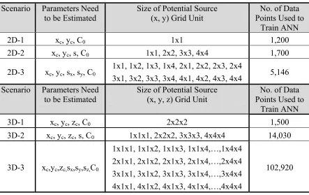
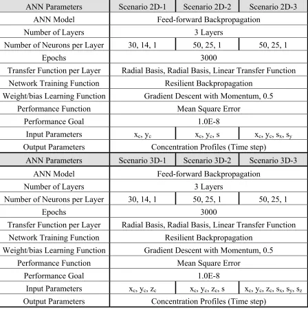
3.4.3 ANN Surrogate Model Settings Used to Develop the Applications Scenarios ...51
3.4.3.1 Data ...53
3.4.3.2 Model Structures...53
3.4.3.3 Training...53
3.4.3.4 Validation...54
3.5 Results and Discussion ...57
3.5.1 ANN-based Surrogate Model Solution Quality...57
3.5.1.1 Two-Dimensional Solution Quality...58
3.5.1.2 Three-Dimensional Solution Quality...59
3.5.2 Contaminant Source Identification Problem Solution ...60
3.5.2.1 Solution of the Two-Dimensional Problem Scenarios...63
3.5.2.2 Solution of the Three-Dimensional Problem Scenarios...66
3.5.3 Timing Study Analysis ...73
3.6 Final Remarks ...73
Chapter 4 ...75
Efficient GA-Based Embedded Hybrid Optimization Methods...75
4.1 Introduction...76
4.2 Optimization Methodologies Background...79
4.2.1 Hybrid Methods Classification ...79
4.2.2 Global and Local Methods Overview ...83
4.2.2.1 Global Search - Genetic Algorithms...83
4.2.2.2 Local Search - Hooke-Jeeves Method ...84
4.2.2.3 Local Search - Powell’s Conjugate Direction Method ...86
4.3 Embedded Hybrid Methods ...87
4.3.1 GA with Hooke-Jeeves’ Search – GA(HJ) ...87
4.3.2 GA with Powell’s Search – GA(Pow) ...88
4.3.3 Local GA Procedure – GA(Local)...89
4.4 Illustrative Application ...90
4.4.1 Application Description ...90
4.4.2 Problem Domain and Simulator Settings...94
4.4.3 Search Parameters Settings ...95
4.5 Results and Discussion ...96
4.6 Final Remarks ...105
Chapter 5 ...107
Noisy GA-Based Search to Address Uncertainty in Real-World Inverse Problems ...107
5.1 Introduction...108
5.2 Groundwater Characterization Problem ...110
5.3 Methodologies: Noisy Genetic Algorithms Optimization ...113
5.3.1 Standard Noisy Genetic Algorithms ...113
5.3.2 Archived Noisy Genetic Algorithms...114
5.4 Numerical Experiments ...116
5.4.1 Illustrative Case Studies...116
5.4.2 Simulator Settings...119
5.4.3 Optimization Model ...119
5.4.4 Setting for the Search Algorthims...121
5.5 Results and Discussion ...122
5.5.1 Case Study 1 ...125
5.5.2 Case Study 2 ...128
6.1 Introduction...135
6.2 Computational Framework Architecture ...138
6.2.1 Simulation Model -- Groundwater Transport Model...139
6.2.1.1 Numerical Methodology ...139
6.2.1.2 Parallel Implementation...139
6.2.2 Optimization Approach – Genetic Algorithms ...141
6.2.3 Adaptor ...142
6.2.4 Framework Parallelism ...143
6.3 Illustrative Case Study ...144
6.3.1 Application - Source History Reconstruction Problem...144
6.3.2 Simulation Model Settings...147
6.3.3 Computational Framework Infrastructure and Resources ...149
6.4 Preliminary Evaluation ...150
6.5 Results and Discussion ...151
6.5.1 Application Solution Results ...151
6.5.2 Framework Performance Results...153
6.5.2.1 Single Site Runs...155
6.5.2.2 Cross Site Runs...161
6.6 Final Remarks ...164
Chapter 7 ...166
Summary and Conclusions...166
References...170
Appendices...178
Appendix A-I Solution of the Two Dimensional Problem Scenarios with Noise ...179
Appendix A-II Solution of the Three Dimensional Problem Scenarios with Noise...182
Appendix B-I Effect of the Chunk Size...185
LIST OF FIGURES
Figure 2-1. A Schematic of a Simulation-Optimization Approach ...8
Figure 2-2. Hypothetical Three-Dimensional Domain Illustrating the Groundwater Inverse Problem ...11
Figure 2-3. A Schematic of the Simulation Model Parallelization...15
Figure 2-4. A Schematic of the Evolutionary Strategies Procedure, Modified from Beyer (2001)...16
Figure 2-5. Hypothetical Three-Dimensional Domain ...22
Figure 2-6. Concentration Profiles Monitored at Observation Wells 5 and 14 for Homogeneous and Heterogeneous Fields, respectively ...23
Figure 2-7. True and Predicted Source Locations for the Homogeneous and Heterogeneous Cases for Scenario 3D-1 ...27
Figure 2-8. True and Predicted Concentration Profiles at Wells 5 and 14 for the Homogeneous and Heterogeneous Case for Scenario 3D-1...28
Figure 2-9. True and Predicted Source Locations for the Homogeneous and Heterogeneous Cases for Scenario 3D-2 ...29
Figure 2-10. True and Predicted Concentration Profiles at Wells 5 and 14 for the Homogeneous and Heterogeneous Case for Scenario 3D-2...29
Figure 2-11. True and Predicted Source Locations for the Homogeneous and Heterogeneous Cases for Scenario 3D-3 ...30
Figure 2-12. True and Predicted Concentration Profiles at Wells 5 and 14 for the Homogeneous and Heterogeneous Case for Scenario 3D-3...31
Figure 2-13. Variation of the Best and the Worst Values for Prediction Error over the 30 Random Trials for the Homogeneous and Heterogeneous Cases Corresponding to Scenario 3D-2 ...32
Figure 2-14. Computation Time Comparison due to Different Degree of Fine Grained Parallelism (Number of Groups =1, Task/Group=1:1)...33
Figure 2-15. Computation Time Comparison due to Different Degree of Semi-Coarse Grained Parallelism (Procs/Group =1:1, Tasks/Group= 1:1) ...34
Figure 2-16. Computation Time Comparison due to Different Degree of Coarse Grained Parallelism (Groups/Server = 1:1, Tasks/Group = 1:1, Population size = 128, Procs/Group = 1:1) ...35
Figure 3-1. A Schematic Explaining the Contaminant Source Identification Problem...42
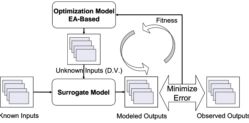
Figure 3-2. Simulation-Optimization Approach Utilizing Surrogate Models ...45
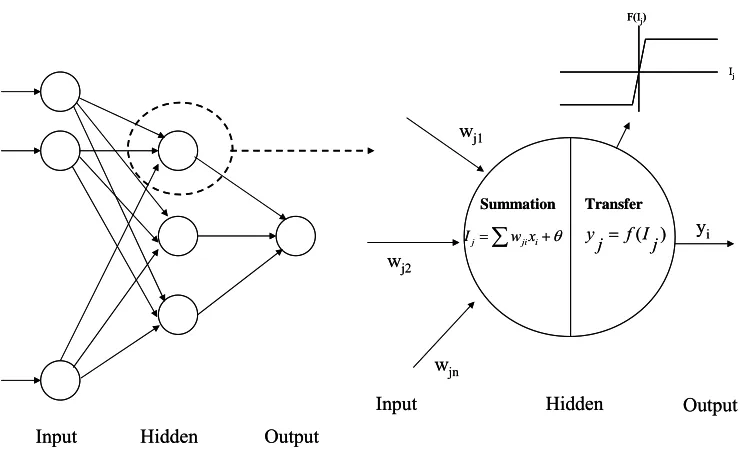
Figure 3-3. Overview of a Typical Feed-Forward Backpropagation ANN ...47
Figure 3-4. Hypothetical Two-Dimensional Domain, Axes Units are Grid Node ...51
Figure 3-5. Hypothetical Three-Dimensional Domain, Axes Units are Grid Node ...52
Figure 3-6. Average Error Values of ANN Models for Scenario 2D-2...57
Figure 3-10. Simulation and ANN Concentration Profiles for Scenario 3D-2 Using Training Data, Profiles are for Source (8, 10, 4, 2, 70) at Wells 1 and 11,
respectively ...60
Figure 3-11. Simulation and ANN Concentration Profile for Scenario 3D-2 Using Test Data, Profiles are for Source (9, 11, 5, 2.5, 70) at Wells 1 and 11, respectively..60
Figure 3-12. Best Source Characterization Solution for Scenario 2D-1 Utilizing Collected Observations from One Well along with Result for 30 Trials...62
Figure 3-13. Source Characterization Solution for Scenario 2D-2 Utilizing Collected Observations from One and Three Wells along with results for 30 trials ...64
Figure 3-14. Source Characterization Solution for Scenario 2D-3 Utilizing Collected Observations from One, Three and Five Wells along with Results for 30 Trials ...65
Figure 3-15. Source Characterization Solution for Scenario 3D-1 Utilizing Collected Observations from Four Wells along with Results for 30 Trials...66
Figure 3-16. Source Characterization Solution for Scenario 3D-2 Utilizing Collected Observations from Four and Nine Wells along with Results for 30 Trials ...68
Figure 3-17. Source Characterization Solution for Scenario 3D-3 Utilizing Collected Observations from Four, Nine and Eighteen Observation Wells with Results for 30 Trials ...69
Figure 3-18. Best and Worst GA Convergence of each Generation for 30 Trials of Scenario 2D-3 Utilizing 5 Observation Wells ...70
Figure 3-19. Best and Worst GA Convergence of each Generation for 30 Trials for Scenario 3D-3 Utilizing 18 Observation Wells ...70
Figure 3-20. Solution Error for all Scenarios...71
Figure 3-21. Solution Error for all Scenarios Using Noisy Observation Data ...72
Figure 4-1. A General Classification of Optimization Methods...80
Figure 4-2. Classification of Hybrid Methods (Architecture Design Issues) , Modified from Talbi (2002) ...81
Figure 4-3. Hypothetical Two-Dimensional Groundwater Domain, Axes Units are Meter....93
Figure 4-4. Convergence Behavior of GA(HJ) Procedure for the Source Identification Problem, Indicated by the Variation of the Best, Average and the Worst Values for Prediction Error over the 30 Random Trials...98
Figure 4-5. Convergence Behavior of GA(Pow) Procedure for the Source Identification Problem, Indicated by the Variation of the Best, Average and the Worst Values for Prediction Error over the 30 Random Trials...98
Figure 4-6. Convergence Behavior of GA(Local) Procedure for the Source Identification Problem, Indicated by the Variation of the Best, Average and the Worst Values for Prediction Error over the 30 Random Trials...99
Figure 4-7. Convergence of the Sequential (GA+HJ) and Embedded GA(HJ) Methods shown by the Variation of the Average Values for Prediction Error over the 30 Random Trials ...99
Figure 4-9. Convergence of the Sequential (GA+Local) and Embedded GA(Local) Methods shown by the Variation of the Average Values for Prediction Error
over the 30 Random Trials ...101
Figure 5-1. Hypothetical Two-Dimensional Groundwater Aquifer, Axes Units are Meter ..112
Figure 5-2. Variation of the Best, the Average and the Worst Values for Prediction Error over the 30 Random Trials for the Three Noisy GA-based Procedures Corresponding to Case Study 1 ...123
Figure 5-3. The Worst, the Average, and the Best Converged Prediction Error Associated with the Maximum and the Minimum Values over the 30 Random Trials for Case Study 1 Utilizing the Noisy Procedures...127
Figure 5-4. Success Rates Associated with the Maximum and the Minimum Values among 30 Trials Utilizing the Noisy Procedures for Case Study 1...128
Figure 5-5. The Best Source Characterization Solution among 30 Trials Utilizing the Noisy Procedures for Case study 1...129
Figure 5-6. The Worst, the Average, and the Best Converged Prediction Error Associated with the Maximum and the Minimum Values over the 30 Random Trials for Case study 2 Utilizing the Noisy Procedures ...131
Figure 5-7. Success Rates Associated with the Maximum and the Minimum Values among 30 Trials Utilizing the Noisy Procedures for Case Study 2...133
Figure 5-8. The Best Source Characterization Solution among 30 Trials Utilizing the Noisy Procedures for Case Study 2 ...133
Figure 6-1. The Framework Overview ...138
Figure 6-2. A schematic of the Simulation Model Parallelization...141
Figure 6-3. A Schematic of Simulation Model Parallelization...144
Figure 6-4. Hypothetical Three-Dimensional Domain ...147
Figure 6-5. Concentration Profiles Monitored at Observation Wells 5 and 14 ...148
Figure 6-6. The TeraGrid Testbed Used...149
Figure 6-7. True and Predicted Concentration for the SHR Problem...153
Figure 6-8. Predicted (Modeled) and True (Observed) Concentration Profiles Monitored at Observation Wells 5...154
Figure 6-9. Fine Grained Parallelism, Number of Groups =1, Task/Group=1:1, Population Size = 128...156
Figure 6-10. Semi-Coarse Grained Parallelism Speedup, Procs/Group =1:1, Tasks/Group= 1:1, Population Size = 128, ** Resources to Run 128 Groups are Not Available at UC/ANL ...157
Figure 6-11. Coarse Grained Parallelism, Groups/Server = 1:1, Tasks/Group = 1:1, Population size = 128, **Resources to Run 32 Servers are Not Available at UC/ANL ...158
Figure 6-12. Coarse Grained Parallelism, Groups/Server = 1:1, Tasks/Group = 1:1, Population Size = 128, ** Resources to Run 32 Servers are Not Available at UC/ANL ...158
Figure 6-15. Cross site runs (Number of Groups vs. Normalized Time for One
Evaluation), Procs/Group =1:1, Tasks/Group= 1:1, Resources to Run 128
Groups are Not Available at UC/ANL ...162 Figure 6-16. Cross site runs (Client-Server vs. Normalized Time for one Generation),
Procs/Group =1:1, Tasks/Group= 1:1, ** Resources to Run 128 Groups are
Not Available at UC/ANL ...162 Figure 6-13A. The effect of Chunk Size Utilizing SDSC Site, Number of Groups = 1,
Population Size = 128, Procs/Group =1:1 ...185 Figure 6-13B. The effect of Chunk Size Utilizing UC/ANL Site, Number of Groups = 1,
Population Size = 128, Procs/Group =1:1 ...185 Figure 6-14A. Scalability Results Utilizing SDSC Site, Procs/Group =1:1, Tasks/Procs =
1:1, Number of Servers =1...186 Figure 6-14B. Scalability Results Utilizing UC Site, Procs/Group =1:1, Tasks/Procs =
LIST OF T
ABLESTable 2-1. Design Variables for Each Scenario...21
Table 2-2. Hypothetical Three-Dimensional Domain Parameters...22
Table 2-3. Common ES Settings Used for the Three Problem Scenarios ...26
Table 2-4. Allowable Range of Decision Variable Values for all Scenarios...26
Table 2-5. True and Predicted Source Characteristics for Scenario 3D-1...27
Table 2-6. True and Predicted Source Characteristics for Scenario 3D-2...28
Table 2-7. True and Predicted Source Characteristics for Scenario 3D-3...30
Table 2-8. Computation Resources Utilized for All Scenarios...35
Table 2-9. Evaluation Time for Each Scenario...37
Table 3-1. Hypothetical Domain Parameters...50
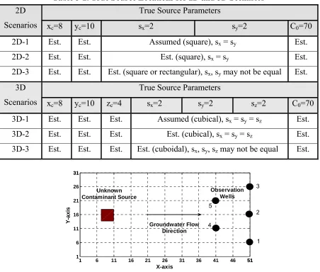
Table 3-2. True Source Locations for 2D and 3D Scenarios...51
Table 3-3. Number and Sizes of Potential Sources for Each Scenario...52
Table 3-4. ANN Model Architecture and Input/Output Parameters...55
Table 3-5. GA Settings for the 2D and 3D Problems ...61
Table 3-6. Allowable Range of Decision Variables Values for 2D and 3D Problems...62
Table 3-7. Best Source Characterization Solution for Scenario 2D-1 Utilizing Collected Observations from One Well ...62
Table 3-8. Best Source Characterization Solution for Scenario 2D-2 Utilizing Collected Observations from One and Three Wells ...63
Table 3-9. Best Source Characterization Solution for Scenario 2D-3 Utilizing Collected Observations from One, Three and Five Wells ...64
Table 3-10. Best Source Characterization Solution for Scenario 3D-1 Problem Utilizing Collected Observations from Four Wells ...66
Table 3-11. Best Source Characterization Solution for Scenario 3D-2 Problem Utilizing Collected Observations from Four Wells ...67
Table 3-12. Best Source Characterization Solution for Scenario 3D-3 Problem Utilizing Collected Observations from Four Wells, Nine Wells and Eighteen Wells...68
Table 3-13. Timing Study for the ANN Surrogate and Simulation Models...72
Table 4-1. Hypothetical Two-Dimensional Domain Parameters...93
Table 4-2. Global Method (GA) Settings ...94
Table 4-3. Local Method Settings ...94
Table 4-4. Sequential Hybrid Method Settings...94
Table 4-5. Embedded Hybrid Method Settings Used for the Problems ...96
Table 4-6. Allowable Range of Decision Variable Values for both Problems...96
Table 4-7. Performance Comparison of the all Nine Methods for Solving the Source Identification Problem ...103
Table 4-8. Performance Comparison of the all Nine Methods for Solving the Combined Problem...104
Table 4-9. The Best Solution Found by each Method for the Source Identification Problem...104
Table 5-3. Allowable Range of Decision Variables Values for both Problems ...122
Table 5-4. The Worst, the Average and the Best Converged Prediction Error among 30 Trials Using the Test Set Utilizing the Noisy Procedures for Case Study 1 ....126
Table 5-5. The Worst, the Average, and the Best Converged Prediction Error among 30 Trials Using the Test Set Utilizing the Noisy Procedures for Case Study 2 ....130
Table 6-1. Hypothetical 3-Dimentional Domain Parameters ...148
Table 6-2. TeraGrid Resources Used...150
Table 6-3. GA Settings Used for the SHR Problem ...152
CHAPTER 1
INTRODUCTION
System characterization using limited observational data collected at measurement stations is generally classified as an inverse problem. Solving inverse problems is relatively complex due to the ill-posedness present in the problem (Sun, 1994). Among several available methods, the simulation-optimization approach is a technique utilized to solve inverse problems by formulating them as an optimization model and solving them by coupling search procedures with the simulation models (Atmadja and Bagtzoglou, 2001). Some simulation models, usually referred to as forward models, are a system of partial differential equations (PDEs) that describes the governing processes of a system and defines the relationships between system inputs and outputs. The inverse problem is solved using a simulation-optimization approach via search algorithms to identify the best system characteristics that minimize the error between the model predictions and the system observations. While this approach is generic and robust, it is computationally expensive as it requires iterative executions of the forward model (Andrad´ottir, 1998).
components: improving the execution efficiency of the simulation model; improving the effectiveness and efficiency of the search algorithms; and facilitating a distributed computational framework to support the simulation-optimization approach.
While evolutionary algorithms (EAs) are good global search procedures, they deem inefficient, when compared with local search procedures, in refining the solutions beyond a certain degree of convergence (Mahinthakumar and Sayeed, 2005). This dissertation research explores new techniques for integrating the good features of the global and local search procedures such that the overall search efficiency is improved. In real-world application, inverse problems occur under noisy environments. Thus, another methodological investigation of this dissertation research is to develop a new algorithm for search under noisy conditions. In addition, recent sciences and technologies have become available through parallel computing and soft computing approaches to expedite the executing time of simulation models. This research investigates techniques to improve the computational efficiency of the simulation model. A fine-grained parallel implementation of the simulation model and a fast surrogate model to approximate the simulation model were also explored.
problems that previously would not have been feasible. Investigations and results based on computational experiments performed on the National Science Foundation’s (NSF’s) TeraGrid demonstrate the efficiency of the grid-enabled simulation-optimization approach in terms of solving accurately the unknown system inputs and improving the computational performance.
Many instances of both research as well as real-world applications are posed as inverse problems. For example, in groundwater contamination characterization problems, the unknown contamination location and the release profile are estimated based on observation data. Similarly, in drinking water distribution system security management, monitoring data from a contamination sensor network is used to determine the contamination potential locations and characteristics so that appropriate evasive actions could be expeditiously determined and executed (Ostfeld and Salomons, 2005). Another application is in medical imaging where the exact properties of internal organs are assessed via non-invasive screening and diagnosis.
contaminant release concentrations are unknown model inputs, which are resolved from a set of spatially and temporally distributed observational data collected at monitoring wells. This dissertation discusses the solution of the groundwater inverse problems in two and three-dimensional groundwater domains.
CHAPTER 2
COMPUTATIONAL SIMULATION-OPTIMIZATION APPROACH FOR
SOLVING INVERSE PROBLEMS
Abstract
Groundwater environmental characterization involves the resolution of unknown
system characteristics from observation data, and is classified as an inverse problem. Inverse
problems are relatively challenging to solve due to natural ill-posedness and computational
intractability. Here we adopt the use of a simulation-optimization approach that couples a
numerical pollutant-transport simulation model with evolution computation algorithms for
solution of the inverse problem. In this approach, the numerical transport model is solved
iteratively during the evolutionary search, which in general can be computationally intensive
since several hundreds to thousands of forward model evaluations are typically required for
solution. Given the potential computational intractability of such a simulation-optimization
approach, parallel computation is employed to ease and enable the solution of such
problems. In this paper, the solution of two groundwater inverse problems will be explored.
The computational experiments were performed on the TeraGrid available on the National
Center for Supercomputing Applications. The results demonstrate the performance of the
parallel simulation-optimization approach in terms of solution quality and computational
2.1 Introduction
Contaminant source identification problems are important in environmental forensics and characterization of contamination for the purposes of regulatory enforcement and liability assessment. In this problem context, source locations and historical contaminant release schedules are unknowns, and are resolved from the spatially and temporally distributed observations collected at contaminant monitoring wells. Such problems, where system characteristics are estimated from sparse observational data, are classified as inverse problems. A forward model, usually represented by a system of partial differential equations (PDEs), describes the transport processes of the groundwater system and defines the relationship between system inputs and outputs. Comprehensive overviews of these types of problems are described by Sun (1994) and Yeh (1986).
In general, inverse problems could be described as problems where the response of the system is known, but not the conditions that led to it. In the context of numerical modeling, finding model input parameter values given output data can be categorized as a problem of time inversion. This means that for time dependent systems, we have to solve the governing equations backward in time through “inverse modeling” (Atmadja and Bagtzoglou, 2001). Inverse problems are generally difficult to solve due to ill-posedness arising from: (1) non-existence; (2) non-uniqueness; and (3) instability of the solution (Sun, 1994). The solution complexity of such problems depends on the amount of observations available and the number of system inputs that must be determined.
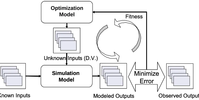
model inputs that best represent the observed data (Figure 2-1). This paper describes the investigation of a simulation-optimization solution approach that employs an evolutionary algorithm-based search method. A simulation-optimization approach to solve an inverse problem is several orders of magnitude more computationally challenging than the solution of the corresponding forward model, since the optimization procedure is based on an iterative process that requires many forward model evaluations.
The computational tractability of such a simulation-optimization approach could be enhanced by improving the efficiency of both the simulation model and the optimization method. Several approaches, such as surrogate modeling and code parallelization, are available to improve the simulation model efficiency by reducing the forward model solution time. In the research presented in this paper, the simulation model parallelism approach is investigated to improve the execution time of the simulation model. This approach is based on high performance computing technologies that are used to expedite the execution time by harnessing the fine and coarse gained parallelism exhibited by the simulation model (Sayeed and Mahinthakumar, 2002).
Observed Outputs Modeled Outputs
Known Inputs
Minimize Error
Optimization Model
Simulation Model
Fitness
Unknown Inputs (D.V.)
Observed Outputs Modeled Outputs
Known Inputs
Minimize Error
Simulation Model
Fitness
Unknown Inputs (D.V.)
The main goal of this research is to enhance the efficiency of the simulation-optimization approach utilizing high performance technologies to reduce the overall computation time for solving inverse problems. This approach is illustrated by applying it to solve instances of a groundwater inverse problem. Many approaches have been considered to solve this problem with varying degree of success. These include regularization and stabilization (e.g., Neupauer et al., 2000), linear programming and multiple regression (e.g., Gorelick et al., 1983), non-linear maximum likelihood estimation (e.g., Wagner, 1992), integer programming (e.g., Mahar and Datta, 1997; 2000; 2001), stochastic differential equations backward in time (e.g., Neupauer and Wilson, 2001), correlation coefficient optimization method (e.g., Sidauruk et al., 1998); and heuristic methods (e.g., Mahinthakumar and Sayeed, 2005; Mirghani et al., 2006). An overview of mathematical methods for groundwater pollution source identification is provided by Atmadja and Bagzogolu (2001).
The following section describes the overall source characterization inverse problem, followed by a description of the solution approach. The subsequent section presents the problem scenarios that were investigated and reported in this paper. The results section presents the quality of the solutions obtained for the different scenarios and computational performance comparisons. The last section provides a summary and presents some observations.
2.2 Problem Overview
illustrates the groundwater source identification problem in a three-dimensional groundwater domain.
Agriculture Fields
Oil & Gas Wells
Landfill
Coal Mines
Observations Wells
Pollution plume Septic Tank
Groundwater Flow Agriculture
Fields
Oil & Gas Wells
Landfill
Coal Mines
Observations Wells
Pollution plume Septic Tank
Groundwater Flow
Figure 2-2. Hypothetical Three-Dimensional Domain Illustrating the Groundwater Inverse Problem
The inverse problem could be posed as a constrained optimization model where the prediction error between the observed and simulated concentrations is minimized. Equation 2-1 illustrates a typical error minimization objective function. Numerous constraints are typically included to enforce decision variable bounds and feasibility.
1 1
minimizenw n obs- sim
ij ij
DV
∑∑
j= i= C C (2-1)where obs i j
C is the observed concentration estimated using the groundwater forward model for
time step i at monitoring well j, n is the number of contamination simulation time steps, nw is the number of monitoring wells, sim
i j
C = f (contaminant source location, size, concentration)
number of contaminant sources, the number of decision variables is equal to the product of the number of contaminant sources times the number of unknowns used to describe each source.
2.3 Solution Approach
The overall simulation-optimization solution framework is developed upon an evolutionary algorithm-based search procedure that is coupled with a parallel groundwater simulation model (i.e., the simulation model in Figure 2-1 is substituted with a parallel groundwater simulation model). Each of the key components of this framework is described in the following subsections.
2.3.1 Simulation Model -- Groundwater Transport Model
The simulation model used as an illustration in solving a groundwater inverse problem in this study is the Parallel Groundwater transport and REMediation code (PGREM3D). This is a suite of massively parallel codes applied for numerical simulation, using the finite element method, of three-dimensional groundwater transport and remediation problems, originally developed by Mahinthakumar (1999). The flow module solves the steady state groundwater flow equation (Bear, 1979) as described below:
(K h) q
∇ ∇ = (2-2)
v K h
θ = − ∇ (2-3)
2.3.1.1 The Transport Governing Equations
The system of equations describing the transport of each dissolved contaminant i(i = 1, 2, …, nc, where nc is the total number of contaminants) undergoing reactions in saturated porous media is defined by
0
( ) ( ) ( ) 1, 2, ...,
i
i i i i i
C q
D C C v C C R i nc
t θ
∂ = ∇ ⋅ ⋅∇ − ∇ ⋅ + − − =
∂ (2-4)
where v is the 3x1 velocity field vector, D is the 3x3 dispersion tensor dependent on v, and Ci
is the dissolved concentration of contaminant i. The term q(Ci-C0i)/θ represents the source
term with volumetric flux q, medium porosityθ, and injected concentration C0i . Ri is the
rate of mass loss of contaminant i due to reactions. More detailed description is provided by Mahinthakumar (1999).
2.3.1.2 Numerical Methodology
2.3.1.3 Parallel Implementation
The transport module simulator codes are written in FORTRAN using double-precision arithmetic. The codes are parallelized using a two-dimensional domain decomposition (in the x and y directions). Explicit message passing interface library (MPI) was utilized to exchange information between these domains. (More details on the use of MPI can be found in many references, such as Gropp et al., 1999). The MPI provides portability to a wide range of parallel architectures, where the use of the MPI communicators is a convenient way to couple processes. The simulation model is implemented to accommodate fine, semi-coarse and coarse grained parallelism. Fine grained parallelism is applied by executing the simulation model on multiple computer processors via the MPI communication library. The semi-coarse grained parallelism is implemented using the MPI Group library, in which multiple instances of the simulation model are executed simultaneously in groups. The coarse grained parallelism is implemented by using multiple servers executed simultaneously; each server consists of a number of groups. This technique is illustrated below considering that a given total number of processors are available. Each server consists of a number of processors equal to [total number of processors/number of servers]. In each server one processor P0SM acts as a server master to establish communication
between the server and the simulator. The remaining number of processors [number of processors in a server-1] will be divided into number of groups. Thus, in each server, each group consists of a number of processors equal to [(number of processors in a server-1) /(number of servers)]. Within each group one processor acts as a group master P0GMto
establish interprocessor communication withP0SM. A schematic of the simulation model
Group 1 P1 P2
P0 Pn PGREM 3D
G.W. Forward Model
Workers processor Group master processor
Interprocessor communication Simulator WORLD COMM. P0 GM Group 2 P1 P2 P0 Pn
Group n P1 P2 P0 Pn
GROUP COMM.
GROUP COMM. GROUP COMM.
Overlapping processor cells Individual processor cells
0 (0,0) 1 (0,1) 2 (0,2) 3 (1,0) 4 (1,1) 5 (1,2) 6 (2,0) 7 (2,1) 8 (2,2)
Interprocessor communication path
G.W. Forward Model Server 1
Server 2
Server n
P0SM
Server WORLD COMM.
P0SM
Server WORLD COMM.
P0SM
Server WORLD COMM.
Simulator Master
Group 1 P1 P2
P0 Pn PGREM 3D
G.W. Forward Model
Workers processor Group master processor
Interprocessor communication Simulator WORLD COMM. P0 GM Group 2 P1 P2 P0 Pn
Group n P1 P2 P0 Pn
GROUP COMM.
GROUP COMM. GROUP COMM.
Overlapping processor cells Individual processor cells
0 (0,0) 1 (0,1) 2 (0,2) 3 (1,0) 4 (1,1) 5 (1,2) 6 (2,0) 7 (2,1) 8 (2,2)
Interprocessor communication path
G.W. Forward Model
Overlapping processor cells Individual processor cells
0 (0,0) 1 (0,1) 2 (0,2) 3 (1,0) 4 (1,1) 5 (1,2) 6 (2,0) 7 (2,1) 8 (2,2)
Interprocessor communication path
G.W. Forward Model Server 1
Server 2
Server n
P0SM
Server WORLD COMM.
P0SM
Server WORLD COMM.
P0SM
Server WORLD COMM.
Simulator Master
Figure 2-3. A Schematic of the Simulation Model Parallelization
2.3.2 Optimization Approach -- Evolutionary Algorithms
Parents
properties encoded in genes
Reproduction
genetic to be mutated
Offspring
new properties by changes genes
Selection
the survival for the fittest
fitness
new fitness mutation
survival destruction
Gen era tio na l lo op Parents
properties encoded in genes
Reproduction
genetic to be mutated
Offspring
new properties by changes genes
Selection
the survival for the fittest
Parents
properties encoded in genes
Reproduction
genetic to be mutated
Offspring
new properties by changes genes
Selection
the survival for the fittest
fitness
new fitness mutation
survival destruction
Gen era tio na l lo op
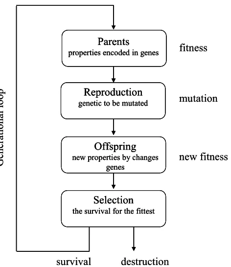
Figure 2-4. A Schematic of the Evolutionary Strategies Procedure, Modified from Beyer (2001)
The simplest form of ES, called (1+1)-ES, operates on a population of size two: the current solution (“parent”) and the offspring of its mutation (“mutant”). If the mutant has a higher fitness than the parent, it becomes the parent in the next generation, otherwise the mutant is discarded. Generally, λ mutants are generated and compete with the parent, this form of ES called (1+λ)-ES. Another form of ES are also available, known as (1,λ)-ES, where the best mutant becomes the parent of the next generation while the current parent is always discarded. The forth form of ES, called (µ/ρ, λ)-ES, usually use a population of µ parents and also recombination as an additional operator. The inherently parallel structure of an ES enables it be used in a parallel and/or distributed computing environment since the fitness evaluation for each individual in a generation can proceed independently, (Schwefel, 1995; Baeck, 1995).
2.3.3 Computational Framework Overview
2.3.3.1 Framework Architecture
Several different search procedures have been implemented, making up the centralized optimization application. Here, the optimization model representation of the inverse problem is solved using evolution strategies. The ES-based procedure encodes, within an individual, the decision variables that describe a potential solution to the inverse problem. The objective function (representing prediction error) of the optimization model is used to quantify a fitness value indicating how well an individual solves the inverse problem. Fitness values are calculated using the results of forward model evaluations. The application of an ES-based search to inverse problems is advantageous because of their robustness and global search characteristics. Some drawbacks, however, include the computational intensity of a typical ES search and the slow final convergence prior to termination.
2.3.3.2 Framework Parallelism
pool used in the framework were designed and implemented as part of Vitri (Baugh, 2003). The master maintains a pool of remote tasks − a bundle of individuals requiring evaluation. Aggregating individuals in this manner reduces communications overhead. Worker processes running on distributed computing resources, having established a TCP-IP socket connection with the master, signal their readiness and draw tasks from the task pool (Mirghani et al., 2005b). The worker process transfers the remote task to the MPI’s zeroth processor. From this point forward, standard MPI group communications are utilized. The forward model manages multiple MPI groups, and each group evaluates an individual in the task bundle. The results of these simulations are then aggregated into a result bundle and returned to the optimization application for processing by the search algorithm. Finally, the subsequent generation of the search is initiated.
2.4 Illustrative Application Setting
In this section, the application problem scenarios along with the optimization formulation for each scenario are explained, and the groundwater fields and the simulation model parameters are described. Also, the optimization formulations for each problem instance are discussed. In addition, the computational framework settings are presented.
2.4.1 Application Scenarios
Three different scenarios were introduced based on how the contaminant source location is characterized. The scenarios were designed to illustrate the problem complexity in terms of the number of unknowns to be estimated and the effect of the groundwater velocity field on estimating these unknowns. In each scenario two cases were considered, namely, homogeneous and heterogeneous hydraulic conductivity fields with the appropriate steady-state hydraulic head and velocity distributions.
For the first scenario (referred to as 3D-1), the contaminant source is characterized by its centroid and contaminant initial concentration, and the simulated contaminant concentration for scenario 1 at a monitoring well is represented as sim1
i j
C = f (xc, yc, zc, C0)
where xc, yc and zc are the coordinates for the centroid of the contaminant source, and C0 is
the initial source concentration.
In the second scenario (referred to as 3D-2), the contaminant source is characterized by the contaminant source location and concentration assuming that the source is cube shaped. Thus, the simulated contaminant concentration for scenario 2 at a monitoring well is represented as sim2
i j
C = f (xc, yc, zc, s, C0) where s is the length of a side of the cube-shaped
Table 2-1. Design Variables for Each Scenario
Scenario Design Variables
3D-1 (xc, yc, zc, C0)
3D-2 (xc, yc, zc, s, C0)
3D-3 (x1, y1, z1, x2, y2, z2, C0)
For the third scenario (referred to as 3D-3), the source is characterized by the contaminant concentration and the coordinates of two diagonally opposite corners of a hexahedron. Thus, the simulated contaminant concentration for scenario 3 at a monitoring well is given by sim3
i j
C = f (x1, y1, z1, x2, y2, z2, C0) where xk, yk and zk (k = 1, 2) are the
coordinates of the vertices of diagonally opposite corners of a hexahedron-shaped source. Table 2-1 summarizes the number of unknowns to be determined for each scenario.
2.4.2 Simulation Setup
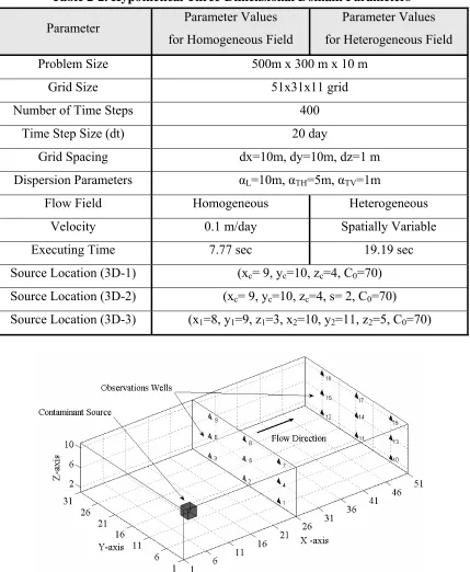
Detailed geometrical and hydraulic parameters are shown in Table 2-2, and in Figure 2-5. Representative simulated concentration profiles at monitoring wells 5 and 14 are shown in Figure 2-6.
Table 2-2. Hypothetical Three-Dimensional Domain Parameters
Parameter Parameter Values for Homogeneous Field
Parameter Values for Heterogeneous Field
Problem Size 500m x 300 m x 10 m
Grid Size 51x31x11 grid
Number of Time Steps 400
Time Step Size (dt) 20 day
Grid Spacing dx=10m, dy=10m, dz=1 m
Dispersion Parameters αL=10m, αTH=5m, αTV=1m
Flow Field Homogeneous Heterogeneous
Velocity 0.1 m/day Spatially Variable
Executing Time 7.77 sec 19.19 sec
Source Location (3D-1) (xc= 9, yc=10, zc=4, C0=70)
Source Location (3D-2) (xc= 9, yc=10, zc=4, s= 2, C0=70)
Source Location (3D-3) (x1=8, y1=9, z1=3, x2=10, y2=11, z2=5, C0=70)
0 0.2 0.4 0.6 0.8
0 1000 2000 3000 4000 5000 6000 7000 8000 Time Steps (days)
Co nc en tr at io n ( m g/ l)
True Concentration, Well 5 True Concnetration, Well 14
0 0.2 0.4 0.6 0.8
0 1000 2000 3000 4000 5000 6000 7000 8000 Time Steps (days)
Co nc en tr at io n ( m g/ l)
True Concentration, Well 5 True Concnetration, Well 14
Homogeneous Heteogeneous
Figure 2-6. Concentration Profiles Monitored at Observation Wells 5 and 14 for Homogeneous and Heterogeneous Fields, respectively
2.4.3 Optimization Models
The contaminant source identification problem is posed as an optimization model where the prediction error denoted by the root squared error (RSE) between the observed and modeled concentrations at a set of monitoring wells is minimized. Equation 2-5 shows the prediction error function used for all scenarios. The constraints represented by Equations (2-6)-(2-11) are included to enforce decision variable bounds and feasibility. Equation 2-6 is applicable to all scenarios, Equation 2-7 is applicable to scenarios 3D-1 and 3D-2, Equations 2-8 and 2-9 are only applicable to scenario 3D-2, and Equation 2-10 and 2-11 are only applicable to scenario 3D-3.
(
)
21 1 minimize sc sc nw n sim obs ij ij
DV
∑ ∑
j= i= C −C (2-5)subject to:
0 ≤ C0 ≤ Cmax (2-6)
xmin ≤ xc ≤ xmax; ymin ≤ yc ≤ ymax; zmin ≤ zc ≤ zmax (2-7)
smin ≤ s ≤ smax (2-8)
xmin ≤ xk ≤ xmax; ymin ≤ yk ≤ ymax; zmin ≤ zk ≤ zmax , k = 1,2 (2-11)
where
DVsc is the set of parameters to be estimated for scenario sc, where,
DV1 = (xc, yc, zc, C0), (2-12)
DV2 = (x
c, yc, zc, s, C0), (2-13)
DV3 = (x
1, y1, z1, x2, y2, z2, C0), (2-14) obs
i
C is the observed concentration at a number of monitoring wells downstream,
sc
sim i
C is the time-series of modeled monitoring concentrations,
xmin, xmax, ymin, ymax, zmin and zmax are the groundwater domain boundaries,
smin and smax are the maximum and minimum source size, respectively,
n is the total number of time steps,
nw is the total number of observations wells.
2.4.4 Computational Resources
The computational experiments presented here were performed on the NSF TeraGrid site. The TeraGrid is a heterogeneous computational resources distributed across the United States connected through a specialized interconnection network designed for high-band width data transfer (Catlett, 2002; 2005). The study was conducted on the IA-64 Intel Itanium2 cluster (1.5 Ghz, 256 computing nodes) available at National Center for Supercomputing Applications (TeraGrid-NCSA) at the University of Illinois at Urbana-Champaign.
2.5 Results and Discussion
when the distributed computational framework is utilized to execute the new solution approach.
2.5.1 Contaminant Source Identification Problem Solution Quality
The results presented here for illustrative purposes are based on synthetically generated observations at the 18 monitoring wells. A “true” conservative contaminant source with a fixed continuous contaminant concentration was placed in the aquifer at a specific location. The groundwater contaminant transport model was executed to generate the concentration profiles at the 18 monitoring wells. These “observed” concentration profiles are used as the observations that should be matched by the source characteristics identified by the simulation-optimization method that minimizes the prediction error function in Eqn. 5. In this study the simulation model is assumed to perfectly generate the concentrations (i.e., no model error), and the measurements have no error.
Since the true source characteristics for these synthetically generated contamination problem scenarios are known, the quality of the identified solutions can be evaluated by comparing them to the known true source characteristics. A solution error metric (Eqn. 2-15) is introduced to evaluate in a post-processing step the quality of the obtained solution.
2
1
- 100
(%)
true pre
n
i i
true
i i
p p
Solution Error
p n
=
⎛ ⎛ ⎞ ⎞
⎜ ⎟
= ⎜ ⎟ ×
⎜ ⎝ ⎠ ⎟
⎝
∑
⎠(2-15)
where pitrue is the true value of unknown (i.e., decision variable) i, pipre is the predicted value
Table 2-3. Common ES Settings Used for the Three Problem Scenarios
Parameter Setting ES Parameter
Scenario 3D-1 Scenario 3D-2 Scenario 3D-3
ES Type ES(µ + λ)
µ 100 100 200
λ 100 100 200
Variables Encoding Real
Number of Generation 49 99 199
Number of Total Evaluations 5,000 10,000 40,000
Several trials were first conducted for each scenario to tweak and fine-tune the ES parameters, such as population size, number of generations, and mutation rate. The common ES parameter settings and the bounds on the decision variables used for the different problem scenarios are shown in Tables 2-3 and 2-4, respectively. As the ES-based search is a probabilistic method, a set of 30 random trials were conducted to evaluate the robustness of the procedure.
Table 2-4. Allowable Range of Decision Variable Values for all Scenarios
Variables Ranges [Minimum, Maximum]
xc, xk [1, 51]
yc, yk [1, 31]
zc, zk [1, 11]
s [1, 10]
C0 [0, 100]
true values. This table also lists the corresponding prediction errors (Eqn. 2-5) and the solution errors (Eqn. 2-7), which indicate good performance (nearly zero prediction error and less than 3% deviation from the true source characteristics) in characterizing the source. Figure 2-7 shows the true and the predicted source locations in the 3D domain for both cases. Figure 2-8 illustrates typical examples of the predicted concentration profiles in comparison to the true concentration profiles at two representative monitoring well locations.
Table 2-5. True and Predicted Source Characteristics for Scenario 3D-1
Homogeneous Case Heterogeneous Case True Value Predicted Value True Value Predicted Value
Variable xc 9 8.72 9 9.45
Variable yc 10 9.94 10 9.68
Variable zc 4 3.92 4 4.33
Variable C0 70 70.00 70 70.12
Prediction Error - 0.000157 - 0.00654
Solution Error (%) - 0.943% - 2.554%
0 0.2 0.4 0.6 0.8
0 2000 4000 6000 8000
Time Steps (days)
C o n c e n tr a tion (m g/l)
True Conc, Well 5 True Conc, Well 14 Predicted Conc, Well 5 Predicted Conc, Well 14
0 0.2 0.4 0.6 0.8
0 2000 4000 6000 8000
Time Steps (days)
Conce n tr at ion ( m g/ l)
True Conc, Well 5 True Conc, Well 14 Predicted Conc, Well 5 Predicted Conc, Well 14
Homogeneous Hetrogeneous
Figure 2-8. True and Predicted Concentration Profiles at Wells 5 and 14 for the Homogeneous and Heterogeneous Case for Scenario 3D-1
In scenario 3D-2, the mutation rate was set to 2.0 and 1.0 for the homogeneous case and heterogeneous case, respectively. Table 2-6 summarizes for both cases the predicted values of the decision variables, which are compared with the corresponding true values, and lists the corresponding prediction and solution errors. The estimated source locations and sizes are shown in Figure 2-9, and a comparison of predicted versus observed concentration values at two representative monitoring wells are shown in Figure 2-10. These results indicate that while the source characterization procedure is able to identify solutions with relatively low prediction errors, the solution error is relatively high (~12%). Most of the error is associated with the estimates for the zc and s parameter values.
Table 2-6. True and Predicted Source Characteristics for Scenario 3D-2
Homogeneous Case Heterogeneous Case True Value Predicted Value True Value Predicted Value
Variable xc 9 9.01 9 9.35
Variable yc 10 9.63 10 9.59
Variable zc 4 2.58 4 3.11
Variable s 2 3.15 2 3.17
Variable C0 70 72.27 70 69.52
Prediction Error - 0.130 - 0.02761
Figure 2-9. True and Predicted Source Locations for the Homogeneous and Heterogeneous Cases for Scenario 3D-2
0 0.2 0.4 0.6 0.8
0 1000 2000 3000 4000 5000 6000 7000 8000
Time Steps (days)
C onc ent ra ti on ( m g/ l)
True Conc, Well 5 True Conc, Well 14 Predicted Conc, Well 5 Predicted Conc, Well 14
0 0.2 0.4 0.6 0.8
0 2000 4000 6000 8000
Time Steps (days)
Conce n tr at ion ( m g/ l)
True Conc, Well 5 True Conc, Well 14 Predicted Conc, Well 5 Predicted Conc, Well 14
Homogeneous Hetrogeneous
Figure 2-10. True and Predicted Concentration Profiles at Wells 5 and 14 for the Homogeneous and Heterogeneous Case for Scenario 3D-2
the presence of non-uniqueness. The 3D-3 scenario in comparison to the 3D-2 and 3D-1 scenarios was computationally more challenging due to the higher degree of non-uniqueness posed by the larger number of unknowns (decision variables).
Table 2-7. True and Predicted Source Characteristics for Scenario 3D-3
Homogeneous Case Heterogeneous Case True Value Predicted Value True Value Predicted Value
Variable x1 8 8.41 8 9.61
Variable y1 9 8.10 9 7.02
Variable z1 3 5.98 3 3.42
Variable x2 10 10.76 10 10.58
Variable y2 11 11.76 11 12.6
Variable z2 5 9.61 5 8.91
Variable C0 70 77.81 70 49.9
Fitness Error - 0.202 - 0.157
Solution Error (%) - 19.53% - 12.99%
0 0.2 0.4 0.6 0.8
0 1000 2000 3000 4000 5000 6000 7000 8000
Time Steps (days)
Conce n tr at ion ( m g/ l)
True Conc, Well 5 True Conc, Well 14 Predicted Conc, Well 5 Predicted Conc, Well 14
0 0.2 0.4 0.6 0.8
0 2000 4000 6000 8000
Time Steps (days)
Conce n tr a ti on ( m g/ l)
True Conc, Well 5 True Conc, Well 14 Predicted Conc, Well 5 Predicted Conc, Well 14
Homogeneous Hetrogeneous
Figure 2-12. True and Predicted Concentration Profiles at Wells 5 and 14 for the Homogeneous and Heterogeneous Case for Scenario 3D-3
0 0.5 1 1.5 2 2.5
0 20 40 60 80 100
Generation Pr e d ic ti o n Er ro r Worst value Best value 0 0.5 1 1.5 2 2.5
0 20 40 60 80 100
Generation Pr e d ic ti o n Er ro r Worst value Best value Hetrogeneous Homogeneous
Figure 2-13. Variation of the Best and the Worst Values for Prediction Error over the 30 Random Trials for the Homogeneous and Heterogeneous Cases Corresponding to
Scenario 3D-2
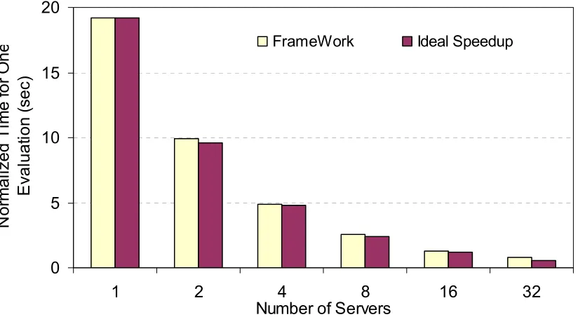
2.5.2 Computational Performance Results
For this comparison, the goal is to measure the overall timing of the simulation-optimization approach for solving the application problem. Different sets of runs were conducted to investigate the performance in terms of fine grained parallelism, semi-coarse grained parallelism and coarse grained parallelism. Since the objective is to evaluate the computational performance, one instance, namely scenario 3D-3 for the heterogeneous case, of the CSI problem was selected for illustrative purposes. A population size of 128 was used for the ES-based procedure, which was executed for 10 generations, to estimate the computing time.
the improvement is limited. Using eight processors or more for such a small problem increases the wall time as a result of excessive communication between processors.
0 5 10 15 20
1 2 4 8 16
Number of Computing Processors per Group
N
o
rm
al
iz
ed
T
im
e
fo
r O
n
e
E
val
u
a
tion
(
se
c)
FrameWork Ideal Speedup
Figure 2-14. Computation Time Comparison due to Different Degree of Fine Grained Parallelism (Number of Groups =1, Task/Group=1:1)
0 5 10 15 20
1 2 4 8 16 32 64 128
Number of Groups
N
o
rm
al
iz
ed T
im
e
fo
r O
n
e
E
val
uat
ion (
sec)
FrameWork Ideal Speedup
Figure 2-15. Computation Time Comparison due to Different Degree of Semi-Coarse Grained Parallelism (Procs/Group =1:1, Tasks/Group= 1:1)
0 5 10 15 20
1 2 4 8 16 32
Number of Servers
N
o
rm
al
iz
ed T
im
e
fo
r O
n
e
E
val
uat
io
n (
sec)
FrameWork Ideal Speedup
Figure 2-16. Computation Time Comparison due to Different Degree of Coarse Grained Parallelism (Groups/Server = 1:1, Tasks/Group = 1:1, Population size = 128,
Procs/Group = 1:1)
Table 2-8. Computation Resources Utilized for All Scenarios
Parameters Values
Number of Clients (Optimizer) 1
Number of Servers (Coarse Grained) 4
Number of Groups (Semi-Coarse Grained) 32 Number of Processors per Group (Fine Grained) 1
Total Number of Nodes (Processors) 73 (146)
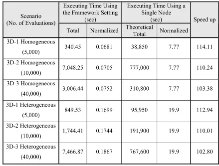
For each scenario, these evaluations were distributed among four servers, each utilizing a 32 processor parallel forward simulation model groups with a single processor per group. Thus, each study utilized a total of 73 computing nodes, i.e., a single node is assigned for the optimization engine, four nodes for the servers, and 68 nodes (134 processors) for the groups with masters. Table 2-8 summarizes the allocation of computation resources, and Table 2-9 shows the total and the normalized computation time utilizing the framework in comparison to the theoretical total and the normalized computation time using a single node for each study. In addition, a speedup analysis is shown for each study. For instance, in the 3D-1 heterogeneous case, an evaluation using the framework took approximately 0.1867 second compared to 19.19 second on a single processor, i.e., solving the problem took approximately 125 minutes (7,467 seconds) instead of approximately nine days (767,600 seconds). The speedup results show that the performance of the framework for all studies are approximately 100 times faster compared to the single processor results.
2.6 Final Remarks
challenging and contains multiple local minima, which negatively affects the performance of the search algorithms. The parallelized framework along three levels, coarse and semi-coarse grained at the search algorithm level and fine grained at the forward model level, reduced the evaluation time drastically, to minutes instead of days. For future work, different solution procedures would be attempted for better solution performance such as modeling to generate alternatives and hybrid algorithms for the 3D-3 scenarios. Also the potential sources zone could be constrained further to simplify the search and to reduce the non-uniqueness issue.
Table 2-9. Evaluation Time for Each Scenario
Executing Time Using the Framework Setting
(sec)
Executing Time Using a Single Node
(sec) Scenario
(No. of Evaluations)
Total Normalized Theoretical
Total Normalized
Speed up
3D-1 Homogeneous
(5,000) 340.45 0.0681 38,850 7.77 114.11
3D-2 Homogeneous
(10,000) 7,048.25 0.0705 777,000 7.77 110.24
3D-3 Homogeneous
(40,000) 3,006.44 0.0752 310,800 7.77 103.38
3D-1 Heterogeneous
(5,000) 849.53 0.1699 95,950 19.9 112.94
3D-2 Heterogeneous
(10,000) 1,744.41 0.1744 191,900 19.9 110.01
3D-3 Heterogeneous
CHAPTER 3
ENHANCED SIMULATION-OPTIMIZATION
APPROACH USING
SURROGATE MODELING FOR SOLVING INVERSE PROBLEMS
Abstract
This paper investigates and discusses groundwater system characterization problem
utilizing surrogate modeling. In this inverse problem, the contaminant signals at monitoring
wells are recorded to recreate the pollution profiles. In this study, simulation-optimization
approach is a technique utilized to solve inverse problems by formulating them as an
optimization model, where evolutionary computation algorithms are used to perform the
search. In this approach, the PDE groundwater transport simulation model is solved
iteratively during the evolutionary search, which in general can be computationally
expensive since thousands of simulation model evaluations will be evaluated. To overcome
this limitation, the simulation model is replaced by a surrogate model which is
computationally much faster than the simulation model and yet is relatively accurate.
Artificial Neural Networks (ANN) is used to construct surrogate models that provide
acceptable accuracy performances. The ANN surrogate model, which replaces the PDE
groundwater transport simulation model, is then coupled with an evolutionary computation
search procedure to solve the source identification problem. In this study, two and
three-dimensional problem settings with several experiments scenarios are investigated. The
results will present the quality solution of the ANN surrogate model versus the groundwater
simulation model, the solution of the inverse problem for different experiment scenarios and
3.1 Introduction
Groundwater system characterization is enormously important in real-time forecasting of groundwater pollutant plumes for making effective decisions to protect environmental resources, conduct liability assessment, estimate risk and design disaster mitigation. The characterization of a source of groundwater pollution from sparse observational data collected at measurement stations is generally classified as an inverse problem. Solving inverse problems is relatively complex due to the ill-posed nature of the problem. Solution of an inverse problem may be limited by non-uniqueness, where more than one solution may exist; instability, where the solutions may be overly sensitive to observation errors; or non-existence, where a solution may not exist (Sun, 1994; Atmadja and Bagtzoglou, 2001).
Surrogate modeling is being investigated to address the excessive computational cost resulting from iterative evaluation of the simulation model. Efficiency of the search could be improved by constructing a surrogate model that is able to estimate quickly the simulation model output (Ong et al., 2003). As the level of complexity of a simulation model increases, the effort and resources needed to construct and train a surrogate model increase as well. This increase, however, occurs prior to the iterative search procedure and does not contribute to the computational burden during the simulation-optimization procedure.
an ANN-based approach to estimate hydraulic conductivity and longitudinal dispersion coefficient in stochastic groundwater modeling. Shigidi and Garcia (2003) used ANN approaches to estimate the hydraulic head values in groundwater domains. Singh et al. (2004) presented some preliminary results for identification of unknown pollution sources using an ANN.
The groundwater contaminant source identification problem (CSI) is utilized in this study. The application problem and the solution approach (ANN-GA) used in this paper resembles the work by Datta and Chakrabarty (2003) in which contaminant source identification problem is solved using an ANN-GA approach. While the previous study modeled a two-dimensional groundwater fields, this work tests both two and three-dimensional heterogeneous flow field problems with increasing problem complexity. Additionally, previous work considered only a few sites as potential source locations, and this study allows 80% of the domain as potential source locations. This study demonstrates the accuracy of the ANN surrogate model in predicting pollutant concentration profiles compared with those produced from the original groundwater transport simulation model. The results also illustrate the quality solution of the inverse problem under alternate scenarios. Finally, a comparative timing study analysis will be demonstrated using the surrogate model versus the simulation model.
3.2 Problem Complexity and Solution Approach
resolved from spatially and temporally distributed concentration observations collected at monitoring wells (Fig. 3-1). The contaminant source locations and the contaminant release at the sources are unknown. Concentration observations at monitoring wells are collected to generate a concentration time-series at each monitoring location. Furthermore, the signature of the source embedded in the monitoring data is a function of the source characteristics.
Observation Wells
Contaminant Plume at time (t) -Concentrations (C)
-Source Location
C Observation Wells
Contaminant Plume at time (t) -
-Source Location
C
Contaminant Plume at time (t) -Source Location
C
Figure 3-1. A Schematic Explaining the Contaminant Source Identification Problem
The inverse problem can be posed as a constrained optimization model where the error between the observed and simulated concentrations is minimized. Several error objective functions can be used to minimize the error; for example Equation 3-1 shows a normalized root square error used to minimize the objective function.
(
)
( )
2
1 1
( ) 2
1 1 -minimize nw n o m iw iw w i nw n
Decision Variables o
iw w i C C C = = = =
∑∑
∑∑
(3-1)where o iw
C is the observed concentration generated using the groundwater forward model for
n readings at discrete time steps recorded at (nw) monitoring wells, m iw
concentrations generated using decision variables as inputs for the groundwater forward model for n readings at discrete time steps modeled at (nw) monitoring wells, and Decision Variables are the contaminant source location(s) and contaminant concentration(s).
3.2.2 Simulation-Optimization Methodologies
Several solution methods for inverse problems, including simulation-optimization techniques, probabilistic procedures, analytical methods, and direct inversion approaches are available (Johnson and Rogers, 2000). This research explores the simulation-optimization approach. This is a general term used to describe optimization techniques that utilize simulation models for the evaluation of objective and constraint functions. In this approach, the simulation model is coupled with optimization techniques to determine the model inputs that best approximate the observed data. This process is applied iteratively until certain stopping criteria are met.
A simulation-optimization approach to solve the groundwater inverse problem is several orders of magnitude more computationally challenging than the solution of the corresponding groundwater transport forward model, since several thousands of forward model evaluations, requiring solution to a system of PDEs, are required, (Andradóttir, 1998). Given the potential computational intractability of such a simulation-optimization approach, improving the efficiency of simulation model is required in this research.