Performance Analysis of Wireless Sensor Network Lifetime Using Queue Length Detection Technique

(1)

ISSN (Print) : 2320 – 3765 ISSN (Online): 2278 – 8875

I

nternational

J

ournal of

A

dvanced

R

esearch in

E

lectrical,

E

lectronics and

I

nstrumentation

E

ngineering

(An ISO 3297: 2007 Certified Organization)

Website: www.ijareeie.com

Vol. 6, Issue 5, May 2017

Performance Analysis of Wireless Sensor

Network Lifetime Using Queue Length

Detection Technique

Noopur Sharma1, Chhabilal Singh2

M. Tech Scholar, Dept. of Electronics Engineering, Shobhit University, Meerut, Uttarpradesh, India1

Assistant Professor, Dept. of Electronics Engineering, Shobhit University, Meerut, Uttarpradesh, India2

ABSTRACT: In order to save energy consumption in wireless sensor network in idle states, on off operation is widely used in wireless Sensor Networks (WSNs), where each node periodically switches between sleeping mode and awake mode. Although efficient toward saving energy, on off causes many challenges, such as difficulty in neighbor discovery due to asynchronous wakeup/sleep scheduling, time-varying transmission latencies due to varying neighbor discovery latencies, and difficulty on multihop broadcasting due to non-simultaneous wakeup in neighborhood. This paper focuses on a novel technique of queue detection method to observe the length of array to be transmitted.

KEYWORDS:Wireless sensor networks, duty cycle, network coding, Upper bound lifetime, energy consumption.

I. INTRODUCTION

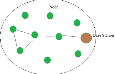
Wireless Sensor Networks (WSN) consist of spatially distributed autonomous sensor nodes which are organized into a cooperative network [1]. WSNs are usually deployed to monitor physical or environmental properties, such as temperature, vibration, pressure, motion, or pollutants. The development of WSNs was initially motivated by military applications such as battlefield surveillance. However, they are increasingly being used in many industrial and civilian application domains, including industrial process monitoring and control [2], machine health monitoring [3], environment and habitat monitoring [4], and medical diagnostics [5]. In WSNs, each node consists of a micro-processor, multiple types of memory (program, data and flash memories), RF transceiver, various sensors and actuators, and power supplies (e.g., batteries and solar cells). A WSN commonly constitutes a wireless ad-hoc

network, that means that every device node supports a multihop routing rule, and several

other nodes might forward knowledge packets to a base station via a sink node. A typical multihop design for WSNs is shown in Fig. 1.

(2)

I

nternational

J

ournal of

A

dvanced

R

esearch in

E

lectrical,

E

lectronics and

I

nstrumentation

E

ngineering

Vol. 6, Issue 5, May 2017

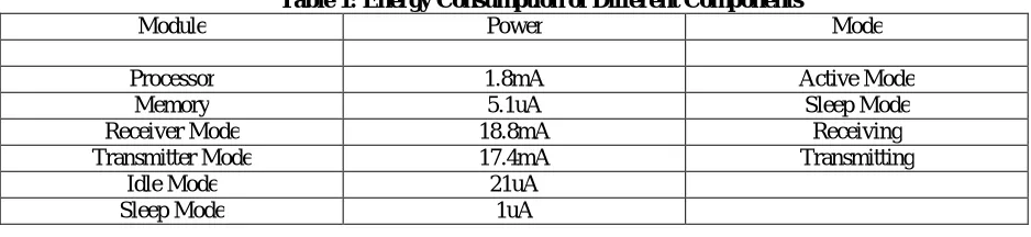
It has been observed that idle energy plays an important role for saving energy in WSNs [6]. Most existing radios [7] used in WSNs support different modes, such as transmit/receive mode, idle mode, and sleep mode. In the idle mode, the radio is not communicating but the radio circuitry is still turned on, resulting in energy consumption which is only slightly less than that in the transmitting or receiving states. Thus, a better way is to shut down the radio as much as possible in the idle mode [6]. The typical energy consumption parameters [8] are shown in Table 1.

Table 1: Energy Consumption of Different Components

Module Power Mode

Processor 1.8mA Active Mode

Memory 5.1uA Sleep Mode

Receiver Mode 18.8mA Receiving

Transmitter Mode 17.4mA Transmitting

Idle Mode 21uA

Sleep Mode 1uA

II. RELATED WORK

Energy may be a terribly thin resource for detector systems and should be managed reasonably so as to increase the lifetime of the detector nodes. Several works are done to cut back the facility consumption and lifelong of wireless detector networks. Generally two main sanctioning techniques area unit known i.e. duty sport and data- driven approaches. Duty sport [9] is that the simplest energy-conserving operation within which whenever the communication isn't needed, the radio transceiver is placed within the sleep mode.

To increase the energy potency of the detector nodes several connected works are done. Honghai Zhang et. al [10] derived associate formula supported the derived bound, associate formula that sub optimally schedules node activities to maximize the time period of a detector network. In [10], the node locations and 2 higher bounds of the time period area unit allotted. Supported the derived bound, associate formula that sub optimally schedules node activities to maximize the time period of a detector network is meant. Simulation results show that the planned

formula achieves around ninetieth of the derived bound. MS Pawar et. al [11] mentioned the impact on time period, and energy consumption throughout listen (with completely different knowledge packet size), transmission, idle and sleep states. The energy consumption of WSN node is measured in several operational states, e.g., idle, sleep, listen and transmit. These results area unit won’t to calculate the WSN node time period with variable duty cycle for sleep time. They finished that sleep current is a vital parameter to predict the life time of WSN node. Almost 79.84% to 83.86% of

total energy is consumed in sleep state. Reduction of WSN node sleep state current I_sleep from 64μA to 9μA has

shown improvement in time period by 193 days for the 3.3V, 130mAh battery. It’s conjointly analyzed that the WSN node time period conjointly depends on the packet size of knowledge.

(3)

I

nternational

J

ournal of

A

dvanced

R

esearch in

E

lectrical,

E

lectronics and

I

nstrumentation

E

ngineering

Vol. 6, Issue 5, May 2017

the constant duty cycle technique. Muralidhar Medidi and Yuanyuan dynasty [13] provided a differential duty cycle approach that's designed supported energy consumed by each traffic and idle listening. It assigns completely different duty cycles for nodes at different distances from the bottom station to deal with the energy-hole downside, improve network time period, and conjointly to take care of network performance. In [13], Francesco Zorzi et. al analyzed the impact of node density on the energy consumption in transmission, reception and idle–listening in a very network wherever nodes follow an obligation cycle theme. They thought-about the energy performance of the network for various eventualities, wherever a completely different range of nodes and different values of the duty cycle area unit taken into consideration. In [15], Joseph Polastre et. al planned B-MAC i.e. a carrier sense media access protocol for wireless detector networks, that has a versatile interface to get ultra-low power operation, high channel utilization and effective collision shunning. B-MAC employs associate adaptive preamble sampling theme to cut back duty cycle and minimize idle paying attention to deliver the goods low power operation. They compared B-MAC to traditional 802.11- galvanized protocols, specifically S-MAC. B-MAC’s flexibility leads to improved packet delivery rates, latency, throughput, and energy consumption than S-MAC.

III ENERGY CONSUMPTION MODELLING

The lifetime of the nodes is evaluated by the overall energy consumption of the nodes such as in [12]. If the energy consumption decreases, then the lifetime of the nodes is increased. The total energy consumed by the nodes consists of

the energy consumed for receivingE , transmitting E , listening for messages on the radio channel (E ), sampling

data (E ) and sleeping (E ).

Total energy consumed is given by

E = E + E + E + E + E (1) Energy consumption by a source node per second across a distance d with path loss exponent n is,

E = D (l + l d ) (2)

Where D is the transceiver relay data rate, l is the energy consumed per bit by the transmitter electronics and l is the

energy consumed per bit in transmit.

Total energy consumption in time t (i.e. duration [0,t]) by a source node (leaf node)

E = t[d (r e + E ) + (1−d )E ) (3) The energy consumption per second by an intermediate node

E = D (l + l d + l ) (4)

Where l is the energy consumed by the sensor node to receive a bit.

Total energy consumption till time t by a relay node is

E = t[d (r e + E ) + (1−d )E ) (5)

IV. LIFETIME UPPER LIMIT

The total energy consumption in the bottleneck zone in time t for a d duty-cycle WSN is given by

E = Nd r t l + Nd r e t + Nd πD + (1−d )tN E (6)

t≤ = T D (7)

Where T upper limit of lifetime and the term is K is given by

(4)

I

nternational

J

ournal of

A

dvanced

R

esearch in

E

lectrical,

E

lectronics and

I

nstrumentation

E

ngineering

Vol. 6, Issue 5, May 2017

V. RESULTS & DISCUSSION

To analyses the performance of wireless sensor network two key parameters are calculated for different techniques and their results are compared. One of the parameter is energy consumption of sensor network and other parameter is lifetime of wireless sensor network. Wireless sensor network energy parameters are shown in table 2.

Table- 2: Network Parameters

Number of Nodes in network 200

Sensor Network Area (A) 100x100

CH nearby radius 30m

Path Loss Exponent 2

l1 1uj

l2 0.8uj

l3 0.5uj

Sleep 30uj

No. of Bits 1000

Battery Energy 25

Hop Length 2m

Threshold Value 8

(5)

I

nternational

J

ournal of

A

dvanced

R

esearch in

E

lectrical,

E

lectronics and

I

nstrumentation

E

ngineering

Vol. 6, Issue 5, May 2017

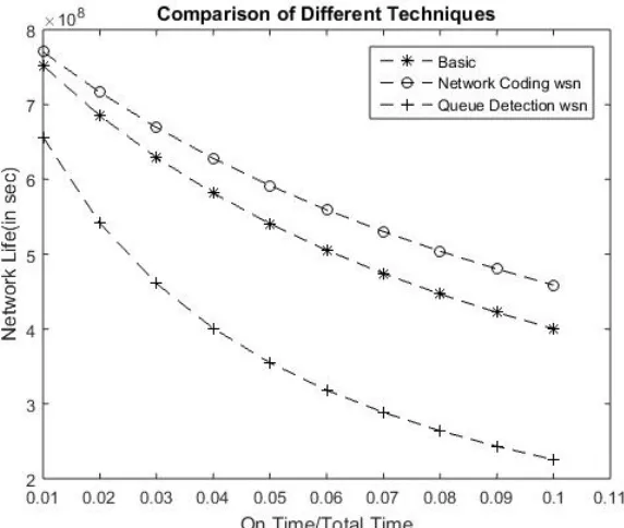
Table 3 and fig.2 shows the lifetime comparison basic wsn, network coding wsn and queue detection based wsn. After observing lifetime values for above three techniques it can be conclude that queue detection technique is best technique to improve network lifetime.

Table3: Lifetime comparison for different techniques

Lifetime for p=0.01

Lifetime for p=0.1

Basic WSN 6.56 x10^8 2.25 x10^8

Network Coding 7.5 x10^8 4.24 x10^8

Proposed WSN 7.8x10^8 4.9 x10^8

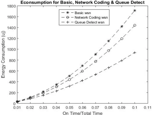
Fig. 3 shows energy consumption in wireless sensor network with change in on off time scheduling. When on off timing ratio value is 0.01, energy consumption is minimum i.e. 28.4uJ, and for on off timing ratio 0.1, energy consumption is more than 1000uJ. With increase in on off timing ratio increases energy consumption decreases. In fig. 3 energy consumption for basic wsn, network coding wsn and proposed wsn is compared. From table 4 it can be conclude that energy consumption for queue detect wsn is minimum.

Fig. 3 Energy Consumption of Sensor Network for Different Techniques

From the fig.3 it is observed that energy consumption is maximum for random duty cycled wsn. Table 4 compares energy consumption for different techniques.

(6)

I

nternational

J

ournal of

A

dvanced

R

esearch in

E

lectrical,

E

lectronics and

I

nstrumentation

E

ngineering

Vol. 6, Issue 5, May 2017

Table4: Energy Consumption for different Techniques

WSN Techniques Energy Consumption for

p=0.01

Energy Consumption for p=0.1

Basic WSN 28.4 1770

Network Coding WSN 28.2 1405

Proposed WSN 27.04 840

VI. CONCLUSION

In this research paper performance of wireless sensor network using different lifetime improvement technique is analyzed and compared. One of the technique is nonscheduled on off timing of motes second technique is network coding technique which used to avoid redundant information received at base station and third technique is a novel technique which is used to set a schedule for motes when they will send data and they will be in sleep mode. An increment of 15.9% over basic wsn and 3.85% over network coding is achieved using proposed technique.

REFERENCES

[1] I. F. Akyildiz, W. Su, Y. Sankarasubramaniam, and E. Cayirci, “Wireless sensor networks: a survey,” Computer Networks, vol. 38, pp. 393–422, 2002.

[2] G. Platt, M. Blyde, S. Curtin, and J. Ward, “Distributed wireless sensor networks and industrial control systems - a new partnership,” in Proceedings of the 2nd IEEE workshop on Embedded Networked Sensors (EmNets05: ), Washington, DC, USA, 2005, pp. 157–158.

[3] A. Mainwaring, D. Culler, J. Polastre, R. Szewczyk, and J. Anderson, “Wireless sensor networks for habitat monitoring,” in Proceedings of the 1st ACM international workshop on Wireless sensor networks and applications (WSNA02: ), 2002, pp. 88–97.

[4] T. He, P. Vicaire, T. Yan, L. Luo, L. Gu, G. Zhou, R. Stoleru, Q. Cao, J. A. Stankovic, and T. Abdelzaher, “Achieving real-time target tracking using wireless sensor networks,” in Proceedings of the 12th IEEE Real-Time and Embedded Technology and Applications Symposium (RTAS06), 2006, pp. 37–48.

[5] J. A. Stankovic, Q. Cao, T. Doan, L. Fang, Z. He, R. Kiran, S. Lin, S. Son, R. Stoleru, and A. Wood, “Wireless sensor networks for in-home healthcare:,” in Proceeding of High Confidence Medical Devices, Software, and Systems (HCMDSS05), 2005, pp. 2–3.

[6] L. M. Feeney and M. Nilsson, “Investigating the energy consumption of a wireless network interface in an ad hoc networking environment,” in IEEE Conference on. Computer Communications (INFOCOM), 2001, pp. 1548–1557.

[7] T. I. (TI), “Cc2420 data sheet,” http://focus.ti.com/lit/ds/symlink/cc2420.pdf.

[8] Crossbow, “Telosb datasheet,” http://www.xbow.com/Products/Product pdf files/Wireless pdf/TelosB Datasheet.pdf.

[9] E. Y. A. Lin, J. M. Rabaey, and A. Wolisz, “Power wireless sensor networks,” Proceedings of the IEEE International Conference on Communications pp. 3769–3776, June 2004.

[10] Honghai Zhang and Jennifer C. Hou, Maximizing 1(1/2), 2006, pp. 64-71.

[11] MS Pawar, JA Manore, MM Efficient WSN Applications’, IJCST Vol. 2, Iss ue 4, Oct . [12] Yuqun Zhang, Chen-Hsiang Feng Duty Cycle Assignment for Receiver

[13] Muralidhar Medidi, Yuanyuan Zhou, ‘Extending Lifetime with Differential Duty Cycles in Wireless Sensor Networks’, IEEE Communications Socie [14] Francesco Zorzi, Milica Stojanovic Cycle on Energy Efficiency in Underwater Networks’, Conference Europe, 2010.

[15] Joseph Polastre, Jason Hill, David Culler, ‘ Networks’, November 3–5, 2004.

BIOGRAPHY

Chhabilal Singh was born in Satna. Madhyapradesh, on February 1, 1983. He received the M-Tech. degree in Telecommunication System Engineering in 2011, from the IIT Kharagpur, West Bengal. He is working as a Assistant Professor in Electronics and

Communication Engineering Department from August 2011 to till now.