Programmable Hash Functions and Their Applications
Dennis Hofheinz1 and Eike Kiltz2 1
Institut f¨ur Kryptographie und Sicherheit, Karlsruhe Institute of Technology, Germany. Email: [email protected].
2
Fakult¨at f¨ur Mathematik, Ruhr-Universit¨at Bochum. Email:[email protected].
Abstract. We introduce a new combinatorial primitive calledprogrammable hash functions (PHFs). PHFs can be used toprogram the output of a hash function such that it contains solved or unsolved discrete logarithm instances with a certain probability. This is a technique originally used for security proofs in the random oracle model. We give a variety ofstandard model realizations of PHFs (with different parameters).
The programmability makes PHFs a suitable tool to obtain black-box proofs of cryptographic protocols when considering adaptive attacks. We propose generic digital signature schemes from the strong RSA problem and from some hardness assumption on bilinear maps that can be instantiated with any PHF. Our schemes offer various improvements over known constructions. In particular, for a reasonable choice of parameters, we obtain short standard model digital signatures over bilinear maps.
Keywords:Hash functions, digital signatures, standard model.
1
Introduction
1.1 Programmable Hash Functions
A group hash function is an efficiently computable function that maps binary strings into a group G. We propose the concept of aprogrammable hash functionwhich is a keyed group hash function that can behave in two indistinguishable ways, depending on how the key is generated. If the standard key generation algorithm is used, then the hash function fulfills its normal functionality, i.e., it properly hashes its inputs into a group
G. The alternative (trapdoor) key generation algorithm outputs a key that isindistinguishablefrom the one output by the standard algorithm. It furthermore generates some additional secret trapdoor information that depends on two (user-specified) generators g andhfrom the group. This trapdoor information makes it possible to relate the output of the hash function H tog andh: for any inputX, one obtains integersaX
andbX such that the relation
H(X) =gaXhbX ∈
G (1)
holds. For the PHF to be (m, n)-programmable we require thatfor all choices ofX1, . . . , XmandZ1, . . . , Zn
such that for alli, jit is true thatXi6=Zj, it holds thataXi = 0 butaZj 6= 0, with significant probability:
Pr[aX1=. . .=aXm = 0∧aZ1, . . . , aZn6= 0]≥1/poly . (2)
Hence parametermcontrols the number of elementsXfor which we can hope to have H(X) =hbX; parameter
ncontrols the number of elementsZ for which we can hope to have H(Z) =gaZhbZ for somea
Z 6= 0.
The concept becomes useful in groups with hard discrete logarithms and when the trapdoor key generation algorithm does not know the discrete logarithm ofhto the basisg. It is then possible to program the hash function such that the hash images of all possible choicesX1, . . . , Xmofminputs do not depend ong (since
aX = 0). At the same time the hash images of all possible choices Z1, . . . , Zn of n (different) inputs do
depend ongin a known way (sinceaZ 6= 0).
some hash queries can be used to simulate, e.g., a signing oracle for an adversary (which would normally require knowledge of a secret signing key). On the other hand, once the adversary produces, e.g., a signature on its own, our hope is that this signature corresponds to a hash query for which the we do not know the discrete logarithm. This way, the adversary has produced a piece of nontrivial secret information which can be used to break an underlying computational assumption.
This way of “programming” a hash function is very popular in the context of random oracles [6] (which, in a sense, are ideally programmable hash functions), and has been used to derive proofs of the adaptive security of cryptosystems [7,14,12].
An (m,poly)-PHF is an (m, n)-PHF for all polynomialsn. A (poly, m)-PHF is defined the same way. Note that, using this notation, a random oracle implies a (poly,1)-PHF.
Instantiations. As our central instantiation of a PHF we use the following function which was originally introduced by Chaum et. al. [23] as a collision-resistant hash function. The “multi-generator” hash function HMG :{0,1}` →
G is defined as HMG(X) := h0Q
` i=1h
Xi
i , where thehi are public generators of the group
andX = (X1, . . . , X`). After its discovery in [23] it was also used in other constructions (e.g., [19,24,4,65]),
relying on other useful properties beyond collision resistance. Specifically, in the analysis of his identity-based encryption scheme, Waters [65] implicitly proved that, using our notation, HMG is a (1,poly)-programmable hash function. Our main result concerning instantiations of PHFs is a new analysis of HMG showing that it is also a (2,1)-PHF. Furthermore, we can use our new techniques to prove better bounds on the (1,poly )-programmability of HMG. Our analysis uses random walk techniques and is different from the one implicitly given in [65].
Variations.The concept of PHFs can be extended to randomized programmable hash functions (RPHFs). A RPHF is like a PHF whose input takes an additional parameter, the randomness. Our main constructions of a randomized hash functions are RHF and RHL. They are both (1,1)-programmable and have short
parameters. In some applications (e.g., for RSA signatures) we need a special type a PHF which we call bounded PHF. Essentially, for bounded PHFs we need to know a certain upper bound on the|aX|from (1),
for allX.
1.2 Applications
Collision Resistant Hashing. We aim to use PHFs as a tool to provide black-box proofs for various cryptographic protocols. As a toy example let us sketch why, in prime-order groups with hard discrete logarithms, any (1,1)-PHF implies collision resistant hashing. Setting up H using the trapdoor generation algorithm will remain unnoticed for an adversary, but any collision H(X) = H(Z) with X 6= Z gives rise to an equation gaXhbX = H(X) = H(Z) =gaZhbZ with known exponents. Since the hash function is (1,
1)-programmable we have that, with non-negligible probability,aX = 0 andaZ 6= 0 (so in particularaX 6=aZ).
This implies h= gaZ/(bX−bZ), revealing the discrete logarithm of hto the base g. (Note that already the
weaker conditionaX6=aZ is sufficient to imply collision resistance.)
Generic Bilinear Map signatures.We propose the following generic Bilinear Maps signature scheme with respect to a group hash function H. The signature of a messageX is defined as the tuple
SIGBM[H] : sig= (H(X)x1+s, s)∈G× {0,1}η, (3)
wheresis interpreted as a randomη-bit integer, andx∈Z|G|is the secret key. The signature can be verified with the help of the public keyg,gxand a bilinear map. This signature scheme can be seen as a generalization
Generic RSA signatures. We propose the following generic RSA signature scheme with respect to a group hash function H. The signature of a messageX is defined as the tuple
SIGRSA[H] : sig= (H(X)1/e, e)∈ZN × {0,1}η, (4)
whereeis aη bit prime. Theeth root can be computed using the factorization ofN =pqwhich is contained in the secret key. Our main theorem concerning RSA signatures states that if, for some m ≥ 1, H is an (m,1)-programmable hash function and the strong RSA assumption holds, then the above signature scheme is unforgeable against chosen message attacks. Again, the parameter m controls the size of the prime as
η≈30 + 80/m. Furthermore, our generic constructions explain signature schemes by Okamoto [57], Fischlin [33], variants of Zhu [66,67] and Camenisch and Lysyanskaya [21], and shed light why other proposals are not secure.
Other applications.BLS signatures [15] are an example of “full-domain hash” (FDH) signature schemes [6]. Using the properties of a (m,1)-programmable hash function one can give a black-box reduction fromm-time unforgeability ofSIGBLS to breaking the CDH assumption. The same reduction also holds for all full-domain hash signatures, for example also RSA-FDH. Consequently, with a (poly,1) PHF we obtain full unforgeability of full-domain signature schemes. Similarly, the Boneh-Franklin IBE scheme [13] can be proved secure under the Bilinear Diffie-Hellman assumption when instantiated with a (poly,1)-PHF. Unfortunately, we do not know of any standard-model instantiation of (poly,1)-PHFs. This fact may be not too surprising given the impossibility results from [30].3
It is furthermore possible to reduce the security of Waters’ IBE and signature scheme [65] to breaking the CDH assumption, when instantiated with a (1,poly)-programmable hash function. This explains Waters’ specific analysis in our PHF framework. Furthermore, our improved bound on the (1,poly)-programmability of HMG gives a (slightly) tighter security reduction for Waters’ IBE and signature scheme.
1.3 A Conceptual Perspective
We would like underline the importance of programmable hash functions as a concept for designing and analyzing cryptographic protocols in the Diffie-Hellman and RSA setting. The central idea is that one can partition the output of a hash function into two types of instances (c.f. (1) and (2)) that can be treated differ-ently by a security reduction. This is reminiscent to what proofs in the random oracle model usually do (e.g., [7,14,12]) and hence PHFs offer a simple and abstract framework for designing and analyzing cryptographic protocols without explicitly relying on random oracles. More importantly, a large body of cryptographic protocols with security in the standard model are using — implicitly or explicitly — the partitioning trick that is formalized in PRFs. To mention only a few examples, this ranges from collision-resistant hashing [23,4], digital signature schemes [11,65] (also in various flavors [57,61,46,8]), chosciphertext secure en-cryption [18,49,43,44,17], identity-based enen-cryption [9,10,51,22,2] to symmetric authentication [52]. In fact, besides a number of specific proofs, there seem to be only two generic techniques known to prove (Diffie-Hellman and RSA-based) cryptographic protocols in the standard model: the partitioning trick as abstracted in programmable hash functions and the recentdual system approach by Waters [64].
1.4 Short Signatures
Our main new applications of PHFs are short signatures in the standard model. We now discuss our results in more detail. We refer to [15,11] for applications of short signatures.
The birthday paradox and randomized signatures.A signature schemeSIGFischby Fischlin [33] (itself a variant of the RSA-based Cramer-Shoup signatures [28]) is defined as follows. The signature for a message
3
mis given bysig:= (e, r,(h0hr1h
m+rmod 2`
2 )
1/emodN), whereeis a randomη-bit prime andris a random
` bit mask. The birthday paradox (for uniformly sampled primes) tells us that after establishingq distinct Fischlin signatures, the probability that there exist two signatures, (e, r1, y1) onm1and (e, r2, y2) onm2, with thesame prime eis roughlyq2η/2η. One can verify that in case of such a collision, (e,2r1−r2,2y1−y2) is a valid signature on the “message” 2m1−m2(with constant probability). Hence, from two Fischlin signatures w.r.t. the same randomnessea signature can be computed (and hence the scheme can be broken). Usually, for “k bit security” one requires the adversary’s success ratio (i.e., the forging probability of an adversary divided by its running time) to be upper bounded by 2−k. Fork= 80 and assuming the number of signature
queries is upper bounded byq= 230, the length of the prime must therefore be at leastη >80 + 60 + 8 = 148 bits to immunize against this birthday attack. We remark that for a different reason, Fischlin’ signatures even requireη≥160 bits.
Beyond the birthday paradox. In fact, Fischlin’s signature scheme can be seen as our generic RSA signatures scheme from (4), instantiated with a concrete (randomized) (1,1)-PHF (RHF). In our notation, the programmability of the hash function is used at the point where an adversary uses a given signature (e, y1) to create a forgery (e, y) with thesame prime e. A simulator in the security reduction has to be able to computey1 = H(X)1/e but must usey = H(Z)1/e to break the strong RSA challenge, i.e., to compute
g1/e0 and e0 >1 fromg. However, since the hash function is (1,1)-programmable we can program H withg
and h=ge such that, with some non-negligible probability, H(X)1/e =hbX/e=gbX can be computed but
H(Z)1/e= (gaZhbZ)1/e=gaZ/egbZ can be used to break the strong RSA assumption sincea
Z 6= 0.
Our central improvement consists of instantiating the generic RSA signature scheme with an (m, 1)-PHF to break the birthday bound. The observation is that such hash functions can guarantee that after establishing up tomsignatures with respect to the same prime, forging is still impossible. In analogy to the above, with an (m,1)-PHF the simulation is successful as long as there are at mostmmany signatures that use the same prime as in the forgery. By the generalized birthday paradox we know that after establishing
q distinct generic RSA signatures the probability that there exists m signatures with the same prime is roughly qm+1(2ηη)
m. Again, the success ratio has to be bounded by 2−80 for q = 230 which means that SIGRSA[H] instantiated with a (2,1)-PRF can have primes as small as η = 80 bits to be provably secure.4 The security proof for the bilinear map schemeSIGBM[H] is similar. Due to the extended birthday paradox (for uniform random strings),SIGBM[H] instantiated with a (2,1)-PRF only needsη= 70 bits of randomness to be provably secure.
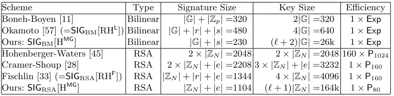
Instantiations. Table 1 compares the signature sizes of our and known signatures assumingq= 230. For RSA signatures our scheme SIGRSA[HMG] offers a short alternative to Fischlin’s signature scheme. More importantly, generating a random 80 bit prime will be considerably faster than a 160 bit one. Concretely, since the complexity of finding a random η-bit prime with error 2−k is O(kη4) we expect that, compared to the one by Fischlin, the signing algorithm of new scheme SIGRSA[HMG] is roughly 16 times faster. Our generic bilinear construction instantiated with the RPHF RHFexplains the signature scheme by Fischlin [33]; instantiated with the the RPHF RHLit explains a variant of the schemes by Zhu [66,67]5and Camenisch and Lysyanskaya [21]. (Concretely, our variant uses a modified randomness space, see Appendix B for details.)
4
A remark in [33, Sec. 2.3] concerning a stateless signature variant that can be securely instantiated with η= 80 bit primes turned out incorrect. Concretely, [33]-signatures are of the form (e, α, y) and satisfyye=xhα1h
α⊕H(m) 2 for publich1, h2, x. In this,eis a 160-bit prime, andα∈ {0,1}160is uniform. The remark in [33, Sec. 2.3] suggests to instead use a signature (e, α, y) with ye = xhα1h
α⊕H1(m)
2 h
α⊕H2(m)
3 forH(m) =: H1(M)||H2(M) and public
h1, h2, h3, x. This has the advantage thate and α can be chosen of size around 80 bits. It is claimed that the security proof of the original scheme can be adapted to this variant. However, the proof crucially uses that there is no collision among theevalues used during the signing process, i.e., that noeoccurs in more than one simulated signature. With 160-bit primese, such a collision will occur only with small probability; but with 80-bit primese, the probability will be in the order of 1/240.
5
The security proof given in [67] does not seem to be correct. Concretely, Zhu’s signatures are of the form (e, α, y) and satisfyye=h0hα1h
H(m)
2 for public h0, h1, h2. In this,eis a random 2k-bit prime, andα∈ {0,1}` is uniform. However, in the security proof of a Type I adversary (for which e=ej ∈ {e1, . . . , eq}), one needs to argue that
Scheme Type Signature Size Key Size Efficiency Boneh-Boyen [11] Bilinear |G|+|Zp|=320 2|G|=320 1×Exp
Okamoto [57] (=SIGBM[RHL]) Bilinear |G|+|r|+|s|=480 4|G|=640 1×Exp
Ours:SIGBM[HMG] Bilinear |G|+|s|=230 (`+ 2)|G|=26k 1×Exp
Hohenberger-Waters [45] RSA 2× |ZN|=2048 2× |ZN|=2048 160×P1024 Cramer-Shoup [28] RSA 2× |ZN|+|e|=2208 3× |ZN|+|e|=3232 1×P160 Fischlin [33] (=SIGRSA[RHF]) RSA |ZN|+|r|+|e|=1344 4× |ZN|=4096 1×P160 Ours:SIGRSA[HMG] RSA |ZN|+|e|=1104 (`+ 1)|ZN|=164k 1×P80
Table 1.Recommended signature sizes of different schemes. The parameters are chosen to provide unforgeability with
k= 80 bits security after revealing maximalq= 230 signatures. RSA signatures are instantiated with a modulus of |N|= 1024 bits, bilinear maps signatures in asymmetric pairings with|G|= logp= 160 bits. We assume without loss
of generality that messages are of size`bits (otherwise, we can apply a collision-resistant hash function first), where
`must be in the order of 2k= 160 in order to providekbits of security. The efficiency column counts the dominant operations for signing. For Bilinear signatures this counts the number of exponentiations, for RSA signaturesk×Pη
counts the number of random η-bit primes that need to be generated. We remark that the Hohenberger-Waters scheme relies only on the (non-strong) RSA assumption but its computational cost is incomparably higher.
In our comparison, we have also included the recent scheme of Hohenberger and Waters [45]. Their scheme has the benefit of relying only on the (non-strong) RSA assumption and having a compact verification key. However, their scheme requires a large number of primality tests and exponentiations during signing and verifying.
The main advantage of our bilinear maps scheme SIGBM[HMG] is its very compact signatures of only 230 bits. This saves 90 bits compared to the short signatures scheme from Boneh-Boyen [11] and is only 70 bits larger than the random oracle BLS signatures. The signature scheme SIGBM[RHL] is exactly the one proposed by Okamoto [57] (which was implicitly introduced in a group signature scheme [35]).
An obvious drawback of our constructions is the size of the public verification key since it includes the group hash keyK. For example, for HMG:{0,1}`→
G,Kcontains`+ 1 group elements, where`= 160. In the bilinear case, that makes a verification key of 26kbits compared to 160 bits from [11]. While these short signatures are mostly of theoretical interest and contribute to the problem of determining concrete bounds on the size of standard-model signatures, we think that in certain applications even a large public-key is tolerable. In particular, our public key sizes are still comparable to the ones of recently proposed lattice-based signatures [54,38,22,17]. Furthermore, even for signatures in the random oracle model, sometimes a relatively large verification key is necessary [31].
We remark that our concrete security reductions for the two generic schemes are not tight, i.e., the reductions roughly lose log(q/δ) bits of security (cf. Theorems 10 and 13). Strictly speaking, a non-tight reduction has to be penalized by having to choose a larger group order. Even though this is usually not done in the literature [28,33], we also consider concrete signature size when additionally taking the non-tight security reduction into account. A rigorous comparison will be done in Section 7.
Related Signature Schemes.Our generic bilinear map signature scheme belongs to the class of “inversion-based” signature schemes originally proposed in [59] and first formally analyzed in [11]. The signature scheme from [57] can be viewed as a special case of our generic bilinear map signature scheme instantiated with a ran-domized PHF. Other related standard-model schemes can be found in [37,16]. We stress that our signatures derive from the above since the message does not appear in the denominator of the exponent. Our generic RSA signature scheme builds on the early work by Cramer and Shoup [28]. The signature schemes from [33] and variants of [21,66,67] can be viewed as a special case of our generic bilinear map signature scheme instantiated with a randomized PHF. Other standard-model RSA schemes are [36,20,26,56,40,29,48,60]. We remark that security proofs for strong RSA based signature schemes are quite subtle and several variants
proposed in the literature contain flawed security proofs. As already explained in Footnote 4, a variant by Fischlin [33, Sec. 2.3] cannot be proved secure. Furthermore, the proof of a scheme proposed by Zhu [66,67] turned out to be incorrect (see Footnote 5) but a close variant with slightly larger randomness space (i.e.,
{0,1}LwithL=`+kinstead ofL=`) can be proved secure using our framework.
1.5 Dedicated vs. Programmable Hash Functions
As argued before, random oracles [6] can be viewed as excellent programmable hash functions. For common applications such as full-domain hash signatures or OAEP, one usually instantiates the random oracle with a fixed, dedicated hash function (such as SHA1 [62]), Therefore, one may ask the question if such concrete hash functions (when used as keyed hash functions) can serve as good programmable hash functions. More concretely, is SHA1 an (m, n)-PRF for parametersm, n≥1?
Even though it seems hard to actually disprove, our intuition says that this is very likely not the case. In fact, one of the key design maxims of hash functions like SHA1 is to destroy all algebraic structure. In contrast, the definition of programmable hash functions requires that there is a relation over an algebraic structure. (I.e., we require that H(X) = gaXhbX over the group
G.) In that sense programmable hash functions formalize an obvious weakness in the random oracle methodology: security proofs making in the random oracle model often use a property of the hash function that is commonly avoided by hash function’s designers. Therefore, we do not recommend to use dedicated hash functions as a PHF.
1.6 Open problems
We show that PHFs provide a useful primitive to obtain black-box proofs for certain signature schemes. We leave it for future research to extend the application of PHFs to other types of protocols. Another interesting direction is to find instantiations of PHFs from different assumptions. For instance, the ideas in [22,2,17] seem conceptually close to programmable hash functions in lattices.
We leave it as an open problem to prove or disprove the standard-model existence of (poly,1)-PHFs. (Note that a positive result would imply a security proof for FDH signatures like [7,15]). Moreover, we are asking for a concrete construction of a bounded (m,1)-PHF form >2.6For example, a (3,1)-PHF could be used to shrink the signature size ofSIGBM[H] to≈215 bits; a bounded (5,1)-PHF would make it possible to shrink the size of the prime inSIGRSA[H] to roughlyη = 60 bits and make signing roughly as efficient as RSA full-domain hash7 (with the drawback of a larger public-key). Finally, a (2,1) or (1,poly)-PHF with more compact parameters would have dramatic impact on the practicability of our signature schemes or Waters’ IBE scheme [65].
2
Preliminaries
2.1 Notation
If x is a string, then |x| denotes its length, while if S is a set then |S| denotes its size. If k ∈ N then 1k denotes the string of k ones. Forn ∈ N, we write [n] shorthand for {1, . . . , n}. If S is a set then s ←$ S denotes the operation of picking an element s of S uniformly at random. We write A(x, y, . . .) to indicate that A is an algorithm with inputs x, y, . . .and by z ← A$ (x, y, . . .) we denote the operation of running A
with inputs (x, y, . . .) and lettingzbe the output. With PPT we denote probabilistic polynomial time. For
random variablesX andY, we write X≡γ Y if their statistical distance is at mostγ.
6
We remark that an earlier version of this paper contained a generalization of RHFto a randomized (m,1)-PHF for any m≥2. However, for our applications it did not turn out to be useful. Since for m≥2 it is not sufficiently bounded (it is only 2`m-bounded), it does not lead to more efficient RSA-based signatures. In the bilinear case, the instantiations with this RPHF are all less efficient than Boneh-Boyen signatures.
2.2 Digital signatures
A digital signature scheme SIG consists of three PPT algorithms. The key generation algorithm inputs a security parameter (in unary representation) and generates a secret signing and a public verification key. The signing algorithm inputs the signing key and a message and returns a signature. The deterministic verification algorithm inputs the verification key and returns accept or reject. We demand the usual correctness property. We recall the definition for unforgeability against chosen-message attacks (UF-CMA), played between a challenger and a forgerF:
1. On input of the security parameter k, the challenger generates verification/signing key, and gives the verification key toF;
2. F makes a number of signing queriesto the challenger; each such query is a messagemi; the challenger
signsmi, and sends the resultsigi toF;
3. F outputs a messagemand a signature sig.
We say that forgerF wins the game ifsig is a valid signature onmand it has not queried a signature onm
before. Forger F (t, q, )-breaks the UF-CMA security ofSIG if its running time is bounded byt, it makes at most q signing queries, and the probability that it wins the above game is bounded by. Finally, SIG is UF-CMA secure if no forger can (t, q, )-break the UF-CMA security of SIG for polynomialt and q and non-negligible (in the security parameterk).
2.3 Pairing groups and the q-SDH assumption
Our pairing schemes will be defined on families of bilinear groups (PGk)k∈N. A pairing groupPG=PGk=
(G,GT, p,ˆe, g) consist of a multiplicative cyclic group G of prime order p, where 2k < p < 2k+1, a mul-tiplicative cyclic group GT of the same order, a generator g ∈ G, and a non-degenerate bilinear pairing ˆ
e: G×G → GT. See [11] for a description of the properties of such pairings. We say an adversary A
(t, )-breaks theq-strong Diffie-Hellman (q-SDH) assumption if its running time is bounded byt and
Pr[(s, gx1+s)← A$ (g, gx, . . . , gx q
)]≥,
where g is a uniform generator ofGandx←$ Z∗
p. We require that inPGtheq-SDH [11] assumption holds
meaning that no adversary can (t, ) break theq-SDH problem for a polynomialtand non-negligible.
2.4 RSA groups and the strong RSA assumption
Our RSA schemes will be defined on families of RSA groups (RGk)k∈N. A safe RSA groupRG=RGk= (P, Q)
consists of two distinct safe primesP andQofk/2 bits. (A safe prime is a prime number of the form 2P0+ 1, where P0 is also a prime.) In our later constructions, we will also use QRN, the cyclic group of quadratic residues modulo an RSA numberN =pq.
We say an adversaryA(t, )-breaks the strong RSA assumption if its running time is bounded by tand
Pr[(e >1, z1/e)← A$ (N =P Q, z)]≥,
wherez←$ ZN. We require that inRG the strong RSA assumption [3,34] holds meaning that no adversary can (t, )-break the strong RSA problem for a polynomialtand non-negligible.
3
Programmable Hash Functions
3.1 Definitions
H = (PHF.Gen,PHF.Eval) for a group family G = (Gk) and with input length ` = `(k) consists of two
PPT algorithms. For security parameterk∈N, a keyK←$ PHF.Gen(1k) is generated by the key generation algorithm PHF.Gen. This key K can then be used for the deterministic evaluation algorithmPHF.Eval to evaluate H viay←PHF.Eval(K, X)∈Gfor anyX ∈ {0,1}`. We write H
K(X) =PHF.Eval(K, X).
Definition 1. A group hash functionH is an (m, n, γ, δ)-programmable hash functionif there are PPT al-gorithmsPHF.TrapGen(the trapdoor key generation algorithm) andPHF.TrapEval(the deterministic trapdoor evaluation algorithm) such that the following holds:
Syntactics: For g, h∈G, the trapdoor key generation(K0, t)←$ PHF.TrapGen(1k, g, h) produces a key K0
along with a trapdoor t. Moreover,(aX, bX)←PHF.TrapEval(t, X)produces integers aX andbX for any
X ∈ {0,1}`.
Correctness: We demandHK0(X) =PHF.Eval(K0, X) =gaXhbX for all generatorsg, h∈
Gand all possible (K0, t)←$ PHF.TrapGen(1k, g, h), for allX ∈ {0,1}`and the corresponding(a
X, bX)←PHF.TrapEval(t, X). Statistically close trapdoor keys: For all generators g, h∈Gand for K←$ PHF.Gen(1k) and(K0, t) $
←
PHF.TrapGen(1k, g, h), the keys K andK0 are statisticallyγ-close:K≡γ K0.
Well-distributed logarithms: For all generators g, h ∈ G and all possible K0 in the range of (the first component of )PHF.TrapGen(1k, g, h), for allX
1, . . . , Xm, Z1, . . . , Zn ∈ {0,1}`such thatXi6=Zj for any
i, j, and for the corresponding (aXi, bXi) ←PHF.TrapEval(t, Xi) and(aZi, bZi) ←PHF.TrapEval(t, Zi),
we have
Pr[aX1 =. . .=aXm= 0 ∧ aZ1, . . . , aZn6= 0]≥δ, (5)
where the probability is over the trapdoor t that was produced along with K0.
We simply say that H is an (m, n)-programmable hash function if there is a negligible γ and a noticeable
δ such that H is (m, n, γ, δ)-programmable. Furthermore, we call H (poly, n)-programmable if H is (q, n) -programmable for every polynomialq=q(k). We say that H is (m,poly)-programmable (resp.(poly,poly )-programmable) if the obvious holds.
We remark that the requirement of the statistically close trapdoor keys is somewhat reminiscent to the concept of “lossy trapdoor functions” [58]. Note that a group hash function can be a (m, n)-programmable hash function for different parametersm, nwith different trapdoor key generation and trapdoor evaluation algorithms.
In our RSA application, the following additional definition will prove useful:
Definition 2. In the situation of Definition 1, we say that H is β-bounded (m, n, γ, δ)-programmable if
|aX| ≤β(k)always.
3.2 Instantiations
As a first example, note that a (programmable) random oracle O (i.e., a random oracle which we can completely control during a proof) is trivially a (c,poly) or (poly, c)-programmable hash function, for any constant c > 0: given generators g and h, we simply define the valuesO(Xi) andO(Zj) in dependence of
theXi andZj as suitable expressionsgahb. (For example, by using Coron’s method [27]: the random oracle
on some input X is defined to be as O(X) :=g∆X·a˜X ·h(1−∆X)˜bX, where∆
X is a random biased coin with
Pr[∆X= 1] := 1/(2q(k)) and ˜aX and ˜bX are uniform values from Z|G|. Then (5) is fulfilled with probability
(1−1/(2q(k)))q(k)·(1/(2q(k)))c≥1/(4q(k))c, meaningOis a (poly, c)-programmable hash function.)
We will now give an example of a programmable hash function in the standard model.
Definition 3 (Multi-Generator PHF).LetG= (Gk)be a group family, and let`=`(k)be a polynomial. Then, HMG= (PHF.Gen,PHF.Eval) is the following group hash function:
– PHF.Eval(K, X)parsesK= (h0, . . . , h`)∈G`+1 andX = (x1, . . . , x`)∈ {0,1}` computes and returns
HMGK (X) =h0
`
Y
i=1
hxi
i
Essentially this function was already used, with an objective similar to ours in mind, in a construction from [65]. Here we provide a new use case and a useful abstraction of this function; also, we shed light on the properties of this function from different angles (i.e., for different values of m and n). In [65], it was implicitly proved that HMG is a (1,poly)-PHF:
Theorem 4. For any fixed polynomial q = q(k) and group G with known order, the function HMG is a (1, q)-programmable hash function withγ= 0andδ= 1/8(`+ 1)q.
The proof builds upon the fact that m = 1 and does not scale in the m-component. With a completely different analysis, we can show that
Theorem 5. For any groupGwith known order, the functionHMG is a(2,1)-programmable hash function
withγ= 0 andδ=Θ(1/`).
Proof. We give only the intuition here and postpone the full (and somewhat technical) proof to Appendix A.1. Consider the following algorithms:
– PHF.TrapGen(1k, g, h) setsa
0=−1 and chooses uniformly and independentlya1, . . . , a`∈ {−1,0,1}and
random group exponents8 b
0, . . . , b`. It setshi =gaihbi for 0≤i≤`and returnsK = (h0, . . . , h`) and
t= (a0, b0, . . . , a`, b`).
– PHF.TrapEval(t, X) parses X = (x1, . . . , x`) ∈ {0,1}` and returns a = a0+P
`
i=1aixi and b = b0+ P`
i=1bixi.
It is clear that this fulfills the syntactic and correctness requirements of Definition 1. Also, since thebi are
chosen independently and uniformly, so are the hi, and the trapdoor keys indistinguishability requirement
follows. It is more challenging to prove (5) (for m = 2, n= 1), i.e., that for all strings X1, X2 and Z1 6∈
{X1, X2}, we have that
Pr[aX1 =aX2 = 0∧aZ1 6= 0] =Θ(1/`). (6)
We will only give an intuition here. First, note that the X1, X2, Z1 are independent of the ai, since they
are masked by the bi in hi =gaihbi. If we view X1 as a subset of [`] (where we definei ∈ X1 iff the i-th componentx1i ofX1 is 1), then the value
aX1=a0+
`
X
i=1
aix1i =−1 +
X
i∈X1
ai
essentially9 constitutes a random walk of length |X
1|+ 1 ≤ `+ 1. Theory says that it is likely that this random walk ends up with an aX1 of small absolute value. That is, for any d with |d| = O(
√ `), the probability thataX1 =dis Θ(1/
√
`). In particular, the probability foraX1 = 0 isΘ(1/
√
`). Now ifX1 and
X2 were disjoint and there was noa0in the sum, thenaX1 andaX2 would be independent and we would get that aX1 =aX2 = 0 with probabilityΘ(1/`). But even ifX1∩X26=∅, and taking into accounta0, we can conclude similarly by lower bounding the probability thataX1\X2 =aX2\X1 =−aX1∩X2.
The additional requirement from (6) thataZ1 6= 0 is intuitively much more obvious, but also much harder to formally prove. First, without loss of generality, we can assume thatZ1⊆X1∪X2, since otherwise, there is a “partial random walk”aZ1\(X1∪X2) that contributes toaZ1 but is independent ofaX1 and aX2. Hence,
8
If|G|is not known, this may only be possible approximately.
9 Usually, random walks are formalized as a sum of independent valuesa
i∈ {−1,1}; for us, it is more convenient to
even when already assumingaX1 =aX2 = 0,aZ1still is sufficiently randomized to take a non-zero value with constant probability. Also, we can assumeZ1not to “split”X1in the sense thatZ1∩X1∈ {∅, X1}(similarly for X2). Otherwise, even assuming a fixed value of aX1, there is still some uncertainty about aZ1∩X1 and hence aboutaZ1 (in which case with some probability,aZ1 does not equal any fixed value). The remaining cases can be handled with a similar “no-splitting” argument. However, note that the fixed “a0 = −1” in theg-exponent of h0 is essential: without it, pickingX1 andX2 disjoint and settingZ1=X1∪X2achieves
aZ1 =aX1+aX2 = 0. A full proof is given in Appendix A.1.
Using techniques from the proof of Theorem 5, we can asymptotically improve the bounds from Theorem 4 as follows (a proof can be found in Appendix A):
Theorem 6. For any fixed polynomial q = q(k) and group G with known order, the function HMG is a (1, q)-programmable hash function withγ= 0andδ=O( 1
q√`).
One may wonder whether the scalability of HMG with respect tom reaches further. Unfortunately, it does not (the proof is in Appendix A):
Theorem 7. Assume `=`(k)≥2. Say|G| is known and prime, and the discrete logarithm problem inG
is hard. ThenHMG is not(3,1)-programmable.
If the group order Gis not known (as will be the case in our upcoming RSA-based signature scheme), then it may not even be possible to sample group exponents uniformly. However, for the special case where
G = QRN is the group of quadratic residues modulo N = pq for safe distinct primes p and q, we can
approximate a uniform exponent with a random element fromZN2. (See, e.g., [28].) In this case, the statistical
distance between keys produced byPHF.Genand those produced byPHF.TrapGenis smaller than (`+ 1)/N. We get the following theorem.
Theorem 8. For the groupG= QRN of quadratic residues modulo N =pq for safe distinct primes pand
q, the function HMG is O(q`)-bounded (1, q,(`+ 1)/N,1/8(`+ 1)q)-programmable as well as O(`)-bounded (2,1,(`+ 1)/N,O(1/`))-programmable.
As is to be expected, one can show that also in case G = QRN, the function HMG is not (3,
1)-programmable.
3.3 Randomized Programmable Hash Functions (RPHFs)
In Appendix B we further generalize the notion of PHFs to randomized programmable hash functions (RPHFs). Briefly, RPHFs are PHFs whose evaluation is randomized, and where this randomness is added to the image (so that verification is possible). We show how to adapt the PHF definition to the randomized case, in a way suitable for the upcoming applications. We also give instantiations of RPHFs for parameters for which we do not know how to instantiate PHFs.
4
Basic applications of PHFs
4.1 Collision resistant hashing
As a warm-up, we can show the natural result that any (non-trivially) programmable hash function is collision-resistant.
Theorem 9. Assume |G| is known and prime, and the discrete logarithm problem inGis hard. LetHbe a
Proof. Fix PPT algorithms PHF.TrapGen and PHF.TrapEval. To show H’s collision-resistance, assume an adversaryA that outputs a collision with non-negligible probability with keysK ←$ PHF.Gen(1k). Now by the key closeness of Definition 1, Awill also do so with keysK0 from (K0, t)←$ PHF.TrapGen(1k, g, h), for
anyg, h. Any collision HK0(X) = HK0(X0) withX6=X0 gives rise to an equation
gahb= HK0(X) = HK0(X0) =ga 0
hb0,
where (a, b) ← PHF.TrapEval(t, X) and (a0, b0) ← PHF.TrapEval(t, X0). (5) states that with non-negligible probability, we havea= 0 anda06= 0, in which case we can compute dlogh(g) = (b−b0)/a0 mod|G|.
Similarly (using Lemma 14), one can show that for a PHF forG= QRN, (1,1)-programmability implies
collision-resistance under the strong RSA assumption. We omit the details.
4.2 Other applications
As already discussed in the introduction, PHFs have other applications.
– A (poly,1)-PHF is sufficient to instantiate the hash function used in full-domain hash signatures like BLS signatures or RSA-FDH. A fair number of other protocols (e.g., the Boneh/Frankin IBE scheme [13]) are based on the same “full-domain hash” properties of the hash function. Unfortunately, we do not know if (poly,1)-PHFs do exist, or not. Similarly, a (m,1)-PHF is sufficient to instantiate the hash function used in full-domain hash signatures like BLS signatures or RSA-FDH and show that they are secure m-time signatures.
– A (1,poly)-PHF is sufficient to instantiate the “hash function” used in Waters’ IBE and signature scheme [65]. In fact, the (1,poly)-PHF HMGis the original hash function Waters used in his IBE scheme. Our new bound from Theorem 6 can be used to improve the bound in the security reduction of Waters’ IBE and signature scheme. We expect that the same improvements can be achieved for schemes based on Waters’ IBE, e.g., [1,5,18,50,53].
5
Generic signatures from Bilinear Maps
5.1 Construction
Let PG = (G,GT, p = |G|, g,eˆ : G×G → GT) be a pairing group. Let n = n(k) and η = η(k) be two
arbitrary polynomials. Our signature scheme signs messages m ∈ {0,1}n using randomness s ∈ {0,1}η.10 Let a group hash function H = (PHF.Gen,PHF.Eval) with inputs from{0,1}n and outputs from
Gbe given. We are ready to define our generic bilinear map signature schemeSIGBM[H].
Key-Generation: Generate PG such that H can be used for the group G. Generate a key for H via
K←$ PHF.Gen(1k). Pick a random indexx∈
Z∗pand computeX =gx∈G. Return the public verification
key (PG, X, K) and the secret signing keyx.
Signing: To signm∈ {0,1}n, pick a randomη-bit integersand computey= H K(m)
1
x+s ∈G. The signature
is the tuple (s, y)∈ {0,1}η×
G.
Verification: To verify that (s, y)∈ {0,1}η×
Gis a correct signature on a given message m, check thats is of lengthη, and that
ˆ
e(y, X·gs) = ˆe(HK(m), g).
10For signing arbitrary bitstrings, a collision resistant hash functionCR:{0,1}∗
→ {0,1}ncan be applied first. Due
Theorem 10. Let Hbe an(m,1, γ, δ)-programmable hash function. LetF be a (t, q, )-forger in the existen-tial forgery under an adaptive chosen message attack experiment withSIGBM. Then there exists an adversary
Athat (t0, 0)-breaks the q-SDH assumption witht0≈t and
≤ q δ·
0+qm+1
2mη +
q p+γ .
We remark that the scheme can also be instantiated in asymmetric pairing groups where the pairing is given by ˆe:G1×G2→GT andG16=G2. We use MNT curves [55] such that the elementy∈G1 from the signature can be represented in 160 bits. (See [11] for more details.) Also, in asymmetric pairings, verification can equivalently check if ˆe(y, X) = ˆe(HK(m)·y−1/s, g). This way we avoid any expensive exponentiation in
G2 and verification time becomes roughly the same as in the Boneh-Boyen short signatures [11]. It can be verified that the following proof also holds in asymmetric pairing groups. (Note that the security assumption also has to be adapted to symmetricq-SDH assumption which is given g1, g1x, . . . , g
(xq)
1 , g2, g2x, it is hard to find a pair (c, g11/(x+c)).)
An efficiency comparison of the scheme instantiated with the (2,1)-PHF HMG from Definition 3 is done in Section 7.
5.2 Proof of Theorem 10
Let F be the adversary against the signature scheme. Throughout this proof, we assume that H is a (m,1, γ, δ)-programmable hash function. Furthermore, we fix some notation. Letmibe thei-th query to the
signing oracle and (si, yi) denote the answer. Letm and (s, y) be the forgery output by the adversary. We
introduce two types of forgers:
Type I: It always holds thats=si for some i. Type II: It always holds thats6=si for alli.
ByF1(resp.,F2) we denote the forger who runsF but then only outputs the forgery if it is of type I (resp., type II). We now show that both types of forgers can be reduced to the (q+ 1)-SDH problem. Theorem 10 then follows by a standard hybrid argument.
Both reductions rely on a trick from [11] that given a q-SDH instance ˜g,˜gx, . . . ,g˜xq, one can efficiently
computeg, gx, together withqrandom solved instances (g1/(x+si), s
i). A new instance of the form (g1/(x+s), s)
for s 6∈ {s1, . . . , sq}, however, can be used to break the q-SDH assumption. For Type II forgers this idea
can be applied more or less directly. For Type I forgers it may happen that there is a m-collision in the simulated randomness, i.e, we haves=si1 =. . . sim, and one has to use the properties of the (m,1)-PHF to
be able to simulate the maximalmsignatures of the form (H(mij)
1/(x+s), s), while using the forger’s output H(m)1/(x+s) to break theq-SDH assumption.
Type I forgers
Lemma 11. Let F1 be a forger of type I that (t1, q, 1)-breaks the existential unforgeability of SIGBM[H].
Then there exists an adversaryA that(t0, 0)-breaks the q-SDH assumption with t0 ≈t and
0≥ δ q
1−
qm+1 2mη −
q p−γ
.
To prove the lemma we proceed in games. In the following, Xi denotes the probability for the adversary
to successfully forge a signature in Gamei.
Game 0. Let F1 be a type I forger that (t1, q, 1)-breaks the existential unforgeability of SIGBM[H]. By definition, we have
Game 1.We now use the trapdoor key generation (K0, t)←$ PHF.TrapGen(1k, g, h) for uniformly selected
generators g, h∈Gto generate a H-key for public verification key ofSIGBM[H]. By the programmability of H,
Pr[X1]≥Pr[X0]−γ. (8)
Game 2. Now we select the random values si used for answering signing queries not upon each signing
query, but at the beginning of the experiment. Since thesi were selected independently anyway, this change
is only conceptual. Let E = Sq
i=1{si} be the set of all si, and let E
i = E\ {s
i}. We also change the
selection of the elements g, h used during (K0, t) ←$ PHF.TrapGen(1k, g, h) as follows. First, we uniformly choose i∗ ∈ [q] and a generator ˜g ∈ G. DefineE∗ = E\ {si∗} and E∗,i = E∗\ {si}. Further, define the
polynomialsp∗(η) =Q
t∈E∗(η+t) and p(η) =
Q
t∈E(η+t) and note that deg(p∗)≤q−1 and deg(p)≤q.
Hence the valuesg= ˜gp∗(x),h= ˜gp(x), andX=gx= ˜gxp∗(x)can be computed from ˜g,˜gx, . . . ,˜gxq. Here the indexx∈Z∗|G|is the secret key of the scheme. We then set
g= ˜gp∗(x)= ˜gQt∈E∗(x+t), h= ˜gp(x)= ˜gQt∈E(x+t).
Note that we can compute (x+si)-th roots fori6=i∗fromgand for allifromh. Unless we are in the unlucky
case thatg orhare not generators (which can only happens ifp(x) = 0) this change is purely conceptual:
Pr[X2]≥Pr[X1]−
q
p. (9)
Observe also thati∗ is independent of the adversary’s view.
Game 3.In this game, we change the way signature requests from the adversary are answered. First, observe that the way we modified the generation ofg andhin Game 2 implies that for anyiwithsi6=si∗, we have
yi= HK0(mi)
1
x+si = gamihbmix+1si
=g˜amiQt∈E∗(x+t)g˜bmiQt∈E(x+t)
x+1si
= ˜gamiQt∈E∗,i(x+t)g˜bmiQt∈Ei(x+t) (10)
for (ami, bmi) ← PHF.TrapEval(t, mi). Hence for i 6= i
∗, we can generate the signature (s
i, yi) without
explicitly knowing the secret keyx, but instead using the right-hand side of (10) for computingyi. Obviously,
this change in computing signatures is only conceptual, and so
Pr[X3] =Pr[X2]. (11)
Observe thati∗ is still independent of the adversary’s view.
Game 4.We now abort and raise eventabortcollif ansioccurs more thanmtimes, i.e., if there are pairwise
distinct indicesi1, . . . , im+1withsi1 =. . .=sim+1. There are
q m+1
such tuples (i1, . . . , im). For each tuple,
the probability for si1 =. . . =sim+1 is 1/2
mη A union bound shows that an (m+ 1)-wise collision occurs
with probability at most
Pr[abortcoll]≤
q
m+ 1
1
2mη ≤
qm+1 2mη .
Hence,
Pr[X4]≥Pr[X3]−Pr[abortcoll]>Pr[X3]−
qm+1
2mη . (12)
Game 5. We now abort and raise event abortbad.s if the adversary returns an s ∈E∗, i.e., the adversary returns a forgery attempt (s, y) with s = si for some i, but s 6= si∗. Since i∗ is independent from the
adversary’s view, we havePr[abortbad.s]≤1−1/q for any choice of thesi, so we get
Pr[X5] =Pr[X4∧ ¬abortbad.s]≥ 1
Game 6. We now abort and raise event abortbad.a if there is an index i with si = si∗ but am
i 6= 0, or if
am= 0 for the adversary’s forgery message. In other words, we raise abortbad.a iff we do not haveami = 0
for alliwithsi =si∗ andam6= 0. Since we have limited the number of suchito min Game 4, we can use
the programmability of H. We hence havePr[abortbad.a]≤1−δfor any choice of the mi andsi, so we get
Pr[X6]≥Pr[X5∧ ¬abortbad.a]≥δ·Pr[X5]. (14)
Note that in Game 6, the experiment never really uses secret keyxto generate signatures: to generate the
yi for si 6= si∗, we already use (10), which requires no x. But if abortbad.a does not occur, thenam
i = 0
wheneversi=si∗, so we can also use (10) to sign without knowing x. On the other hand, ifabortbad.a does
occur, we must abort anyway, so actually no signature is required.
This means that Game 6 does not use knowledge about the secret keyx. On the other hand, the adversary in Game 6 produces (wheneverX6happens, which implies ¬abortbad.a and¬abortbad.s) during a forgery
y= HK0(m)1/(x+s)=
˜
gamQt∈E∗(x+t)˜gbmQt∈E(x+t)
x+1s
= ˜gamp
∗(x)
x+s ˜gbmp∗(x).
Fromy and its knowledge abouthand thesi, the experiment can derive
y0 =
y
gp∗(x)b
m
1/am
= ˜gp
∗(x)
x+s .
Since gcd(η+s, p∗(η)) = 1 (where we interpretη+sandp∗(η) as polynomials inη), we can writep∗(η)/(η+
s) =p0(η) +q0/(η+s) for some polynomialp0(η) of degree at mostq−2 and someq0 6= 0. Again, we can computeg0 = ˜gp0(x). We finally obtain
y00= (y0/g0)1/q0 =
˜
gp
∗(x)
(x+s)−p
0(x)1/q0
= ˜gx+1s .
This means that the from the experiment performed in Game 6, we can construct an adversaryAthat (t0, 0 )-breaks theq-SDH assumption.A’s running timet0is approximatelytplus a small number of exponentiations, andAis successful wheneverX6 happens:
0 ≥Pr[X6]. (15)
Putting (7-15) together yields Lemma 11.
Type II forgers
Lemma 12. Let F2 be a forger of type II that (t2, q, 2)-breaks the existential unforgeability of SIGBM[H].
Then there exists an adversaryAthat(t0, 0)-breaks theq-SDH assumption and an adversaryA∗that(t00, 00) -breaks the discrete logarithm problem in Gsuch thatt0, t00≈t2 and
0+00≥δ·(2−γ).
Note that the discrete logarithm problem is at least as hard as the q-SDH problem, so for Theorem 10, we can assume0≥00 without loss of generality.
For the proof, we again proceed in games. The proof is very similar to the proof for type I forgers, so we will be brief where similarities occur.
Game 0. Let F2 be a type II forger that (t2, q, 2)-breaks the existential unforgeability of SIGBM[H]. By definition, we have
Game 1.We now use the trapdoor key generation (K0, t)←$ PHF.TrapGen(1k, g, h) for uniformly selected
generatorsg, h∈Gto generate a H-key for the public verification key ofSIGBM[H]. By the programmability of H,
Pr[X1]≥Pr[X0]−γ. (17)
Game 2.Now we select the used randomness si used for answering signing queries at the beginning of the
experiment and set E =Sq
i=1{si}. We select the elementsg, h passed to PHF.TrapGen(1k, g, h) as follows:
We uniformly choose a generator ˜g∈G. Define the polynomialp(η) =Qt∈E(η+t) and note that deg(p)≤q.
Hence the valuesg= ˜gp(x) andX =gx= ˜gxp(x) can be computed from ˜g,g˜x, . . . ,˜gxq+1. We choose c∈
Z|G| uniformly and set
g= ˜gp(x), h= ˜gcp(x).
Note that we can compute (x+si)-th roots fromg andhfor alli. These change is purely conceptual:
Pr[X2] =Pr[X1]. (18)
Game 3.We answer all signature requests from the adversary as in Game 3 of the proof of Lemma 11. That is, we use the way that g andhare chosen to avoid having to compute the (x+si)th root. This change is
only conceptual, and we have
Pr[X3] =Pr[X2]. (19)
Game 4.We now abort and raise eventabortlogifam+c·bm= 0 mod|G|for the adversary’s forged message
m. Since we chosecas a uniform exponent and only passgandh=gc(but no further information aboutc) to adversary andPHF.TrapGen, these algorithms break a discrete logarithm problem. In particular, we can construct a suitable (t00, 00)-attackerA∗ on the discrete logarithm problem in
Gthat takesgc as input and computesc=−am/bm mod|G|. This adversary achieves
Pr[X4]≥Pr[X3∧ ¬abortlog]≥Pr[X3]−00. (20)
Game 5.We now abort and raise event abortbad.a ifam (obtained fromPHF.TrapEval(t, m)) is zero for the
adversary’s forgery messagem. The programmability of H directly implies
Pr[X5]≥Pr[X4∧ ¬abortbad.a]≥δ·Pr[X4]. (21)
Now from Game 5, we can now construct an adversaryAon the (q+ 1)-SDH assumption.Atakes inputs ˜
g,g˜x, . . . ,˜gxq+1 and simulates Game 5 with adversary F
2. A uses its inputs as if it was selected by the experiment; note that in Game 5, the secret keyxis not used anymore. Now wheneverF2 outputs a forgery
y with
y= gamhbm
1
x+s =˜g(am+c·bm)Qt∈E(x+t)
x+1s
.
Since we haveam+c·bm6= 0 mod|G|, we can compute a nontrivial root of the challenge ˜g. Therefore, from
y0=ycam+1dbm = ˜g p(x)
x+s
6
Generic signatures from RSA
6.1 Construction
LetG= QRN be the group of quadratic residues modulo an RSA numberN =P Q, whereP andQare safe
primes. Letn=n(k) andη=η(k) be two polynomials. Let a group hash function H = (PHF.Gen,PHF.Eval) with inputs from {0,1}n and outputs from
G be given. We are ready to define our generic RSA-based signature schemeSIGRSA[H]:
Key-Generation: GenerateN =P Qfor safe distinct primesP, Q≥2η+2, such that H can be used for the group G= QRN. K
$
←PHF.Gen(1k). Return the public verification key (N, K) and the secret signing
key (P, Q).
Signing: To signm∈ {0,1}n, pick a randomη-bit primeeand computey= H
K(m)1/e modN.Thee-th
root can be computed usingP andQ. The signature is the tuple (e, y)∈ {0,1}η×
ZN. Verification: To verify that (e, y)∈ {0,1}η×
ZN is a correct signature on a given messagem, check that
eis odd and of lengthη, and thatye= H(m) modN. It is not necessary to check specifically thateis a prime.
Theorem 13. Let H be a β-bounded(m,1, γ, δ)-programmable hash function for boundβ ≤2η andm≥1. LetF be a(t, q, )-forger in the existential forgery under an adaptive chosen message attack experiment with
SIGRSA[H]. Then there exists an adversaryAthat (t0, 0)-breaks the strong RSA assumption with t0≈t and
=Θq
δ
0+qm+1(η+ 1)m
2mη−1 +γ . The proof is similar to the case of bilinear maps (Theorem 10).
Let us again consider the instantiation SIGRSA[HMG] for the (2,1)-PHF HMG. Plugging in the values from Theorem 8 the reduction from Theorem 13 leads to = Θ(q`0) + q32(2ηη+1)−12. As explained in the introduction, forq= 230 andk= 80 bits we are now able to chooseη ≈80 bit primes.
6.2 Proof of Theorem 13
We first state the following simple lemma due to [41].
Lemma 14. Given x, z ∈Z∗n, along with a, b∈Z, such that xa =zb, one can efficiently compute x˜ ∈Z∗n
such that ˜x=zgcd(aa,b).
To prove this lemma one can use the extended Euclidean algorithm to compute integers f, g such that
bf+ag= gcd(a, b). One can check that ˜x:=xfzg satisfies the above equation.
Now let F be the adversary against the signature scheme. Throughout this proof, we assume that H is a (m,1, γ, δ)-programmable hash function. Furthermore, we fix some notation. Letmi theith query to the
signing oracle an (ei, yi) denote the answer. Let m and (e, y) be the forgery output by the adversary. We
introduce two types of forgers:
Type I: It always holds thate=ei for some i. Type II: It always holds thate6=ei for alli.
ByF1(resp.,F2) we denote the forger who runsF but then only outputs the forgery if it is of type I (resp., type II). We now show that both types of forgers can be reduced to the strong RSA problem. Theorem 13 then follows by a standard hybrid argument.
Similar to the q-SDH case, both reductions rely on the standard trick [28] that given an RSA instance
N = pq and ˜g ∈ QRN, one can efficiently compute g ∈ QRN, together with q random solved instances (g1/ei, e
i), for random primes ei. A new instance of the form (g1/e, e) fore6∈ {e1, . . . , eq}, however, can be
used to break the strong RSA assumption. For Type II forgers this idea can be applied more or less directly. For Type I forgers it may happen that there is a m-collision in the simulated random primes, i.e, we have
e=ei1 =. . . eim, and one has to use the properties of the (m,1)-PHF to be able to simulate the maximal
m signatures of the form (H(mij)
1/e, e), while using the forger’s output H(m)1/e to break the strong RSA
Type I forgers
Lemma 15. Let F1 be a forger of type I that (t1, q, 1)-breaks the existential unforgeability of SIGRSA[H].
Then there exists an adversaryA that(t0, 0)-breaks the strong RSA assumption with t0 ≈t and
0≥ δ q·
1−
qm+1(η+ 1)m
2mη−1 −γ
.
To prove the lemma we proceed in games.
Game 0. Let F1 be a type I forger that (t1, q, 1)-breaks the existential unforgeability of SIGRSA[H]. By definition, we have
Pr[X0] =1. (22)
Game 1.We now use the trapdoor key generation (K0, t)←$ PHF.TrapGen(1k, g, h) for uniformly selected generatorsg, h∈QRN to generate a H-key for the public verification key ofSIGRSA[H]. By the
programma-bility of H,
Pr[X1]≥Pr[X0]−γ. (23)
Game 2.Now we select the used primesei used for answering signing queries not upon each signing query,
but at the beginning of the experiment. Since theei were selected independently anyway, this change is only
conceptual. Let E=Sq
i=1ei be the set of all ei, and letEi =E\ {i}. We also change the selection of the
elementsg, hused during (K0, t)←$ PHF.TrapGen(1k, g, h) as follows. First, we uniformly choosei∗∈[q] and
generators ˜g∈Z∗
N,˜h∈QRN. We then setE∗=E\ {ei∗},E∗,i=E∗\ {ei}, and
g= ˜g2Qx∈E∗x, h= ˜hQx∈Ex.
Note that we can extract anei-th root fori6=i∗ fromg and for all ifrom h. Unless none of theei divides
|G|, the induced distribution on g and his the same as in Game 1. Since |G|=|QRN| =P0Q0 for primes
P0= (P−1)/2 andQ0 = (Q−1)/2, and we assumed thatP, Q≥2η+2, however, we have thatei does not
divide|G|(for all i).
Pr[X2] =Pr[X1]. (24)
Observe also thati∗ is independent of the adversary’s view.
Game 3.In this game, we change the way signature requests from the adversary are answered. First, observe that the way we modified the generation ofg andhin Game 2 implies that for anyiwithei6=ei∗, we have
thatyi can be written as
HK0(mi)1/ei = gamihbmi
1/ei
=˜g2amiQx∈E∗x˜hbmiQx∈Ex
1/ei
= ˜g2amiQx∈E∗,ix˜hbmiQx∈Eix.
for (ami, bmi)←PHF.TrapEval(t, mi). Hence fori6=i
∗, we can generate the signature (e
i, yi) without explicit
exponent inversion, but instead using this alternative presentation ofyi. Obviously, this change in computing
signatures is only conceptual, and so
Pr[X3] =Pr[X2]. (25)
Observe thati∗ is still independent of the adversary’s view.
Game 4.We now abort and raise eventabortcollif aneioccurs more thanmtimes, i.e., if there are pairwise
distinct indicesi1, . . . , im+1withei1 =. . .=eim+1. There are
q m+1
such tuples (i1, . . . , im). For each tuple,
the probability for ei1 =. . .=eim+1 is 1/P
m, where P denotes the number of primes11 of length η. Since
P >2η/3(η+ 1) log 2 (see, e.g., [63, Theorem 5.7]), a union bound shows that an (m+ 1)-wise collision occurs
with probability at most
Pr[abortcoll]≤
q
m+ 1
3(η+ 1) log 2 2η
m
≤q
m+1(η+ 1)m
2mη ·
(3 log 2)m
(m+ 1)! <
qm+1(η+ 1)m
2mη−1 . 11
Hence,
Pr[X4]≥Pr[X3]−Pr[abortcoll]>Pr[X3]−
qm+1(η+ 1)m
2mη−1 . (26)
Game 5. We now abort and raise event abortbad.e if the adversary returns ane ∈E∗, i.e., the adversary returns a forgery attempt (e, y) with e = ei for some i, but e 6= ei∗. Since i∗ is independent from the
adversary’s view, we havePr[abortbad.e]≤1−1/qfor any choice of the ei, so we get
Pr[X5] =Pr[X4∧ ¬abortbad.e]≥ 1
qPr[X4]. (27)
Game 6. We now abort and raise event abortbad.a if there is an index i with ei = ei∗ but am
i 6= 0, or if
am= 0 for the adversary’s forgery message. In other words, we raise abortbad.a iff we do not haveami = 0
for alliwithei =ei∗ andam6= 0. Since we have limited the number of such ito min Game 4, we can use
the programmability of H. We hence havePr[abortbad.a]≤1−δfor any choice of the mi andei, so we get
Pr[X6]≥Pr[X5∧ ¬abortbad.a]≥δ·Pr[X5]. (28) Note that in Game 6, the experiment never really needs to invert exponents to generate signatures: to generate the yi for ei 6= ei∗, we already use the method of Game 3, which requires no inversion. But if
abortbad.a does not occur, thenami = 0 wheneverei =ei∗, so we can also use that method to sign without
inversion. On the other hand, if abortbad.a does occur, we must abort anyway, so actually no signature is required.
This means that Game 6 does not use knowledge about the factorization of N. On the other hand, the adversary in Game 6 produces (whenever X6 happens, which implies ¬abortbad.a and¬abortbad.e) during a forgery
y= (HK0(m))1/e=
˜
g2amQx∈E∗x˜hbmQx∈Ex
1/e = ˜g
2amQ
x∈E∗x
e ·˜hbmQx∈E∗x.
Fromy and its knowledge about ˜h, and theei, the experiment can derive
y0= y
˜
hbmQx∈E∗x
= ˜g
2amQ
x∈E∗x e .
We have gcd(2amQx∈E∗x, e) = 1 becauseeis larger than|am|by H’s boundedness, so that Lemma 14 finally
allows to obtain y00= ˜g1/e. Since ˜g was chosen initially independently and uniformly from
Z∗N, this means
that the from the experiment performed in Game 6, we can construct an adversaryAthat (t0, 0)-breaks the strong RSA assumption.A’s running timet0is approximatelytplus a small number of exponentiations, and
Ais successful wheneverX6 happens:
0 ≥Pr[X6]. (29)
Putting (22-29) together yields Lemma 15.
Type II forgers
Lemma 16. Let F2 be a forger of type II that (t1, q, 1)-breaks the existential unforgeability of SIGRSA[H].
Then there exists an adversaryA that(t0, 0)-breaks the strong RSA assumption with t0 ≈t and
0≥ δ
2 ·(2−γ).
Again we proceed in games. The proof is very similar to the proof for type I forgers, so we will be brief where similarities occur.
Game 0. Let F2 be a type II forger that (t2, q, 2)-breaks the existential unforgeability of SIGRSA[H]. By definition, we have
Game 1.We now use the trapdoor key generation (K0, t)←$ PHF.TrapGen(1k, g, h) for uniformly selected generatorsg, h∈QRN to generate a H-key for public verification key ofSIGRSA[H]. By the programmability of H,
Pr[X1]≥Pr[X0]−γ. (31)
Game 2. Now we select the used primes ei used for answering signing queries at the beginning of the
experiment and setE=Sq
i=1ei. We select the elementsg, hpassed toPHF.TrapGen(1k, g, h) as follows: we
choose ˜g∈Z∗N andc∈ZN2 uniformly and set
g= ˜g2Qx∈Ex, h=gc= ˜g2c
Q
x∈Ex.
Note that we can extract anei-th root fromg andhfor alli. These change is purely conceptual:
Pr[X2] =Pr[X1]. (32)
Game 3. We answer all signature requests from the adversary as in Game 3 of the proof of Lemma 15. That is, we use the way thatg andhare chosen to avoid having to invert exponents. This change is only conceptual, and we have
Pr[X3] =Pr[X2]. (33)
Game 4. We now abort and raise event abortbad.e if e divides am+c·bm over the integers. Recall that
|G| = |QRN| = p0q0 for primes p0, q0 with N = (2p0+ 1)(2q0+ 1). Recall also that c is chosen uniformly
fromZN2, so we can write c=c1+c2|G|with 0≤c1<|G|. Note thatc2is statistically 1/N-close to being uniformly distributed over {0, . . . ,bN2−1
p0q0 c} and independent of c1. However, the only information about c released to the adversary and thePHF.TrapGenalgorithm ish=gc and hencec
1=c mod|G|.
We would like to find necessary conditions for abortbad.e. To this end, letd= gcd(bm, e). We first claim
that forabortbad.e, it is necessary thatd6=e. For contradiction, assumed=e. Thene|bmby definition ofd.
Since|am|< eby H’s boundedness, we also havee6 |am+c·bm. Taken together this implies thatedoes not
divide am+c·bm, and hence we have¬abortbad.e. Next, we show that forabortbad.e, we need to have d|am.
Again, assumed6 |am for contradiction. Then,d|c·bmandd|eby definition ofd. Hence,e6 |am+c·bm, and
again¬abortbad.e is implied.
So we can assumed6=eandd|amwithout loss of generality in our analysis ofabortbad.e. Thenabortbad.e is equivalent to
am+c·bm= 0 mode ⇔
am
d + (c1+c2|G|) bm
d = 0 mod
e
d ⇔ c2=−|G|
−1 am
d
b
m
d
−1 +c1
!
,
which occurs with probability at most 1/3 + 1/N due to the distribution of c2. (Note that |G| = p0q0 is invertible modulo e/dsince|p0|,|q0|are prime and longer than e, andbm/d is invertible by construction of
d.) We get
Pr[X4]≥Pr[X3∧ ¬abortbad.e]≥ 2
3− 1
N
Pr[X3]≥ 1
2 ·Pr[X3]. (34)
Game 5.We now abort and raise event abortbad.a ifam (obtained fromPHF.TrapEval(t, m)) is zero for the
adversary’s forgery messagem. The programmability of H directly implies
Pr[X5]≥Pr[X4∧ ¬abortbad.a]≥δPr[X4]. (35)
Now from Game 5, we can now construct an adversary A on the strong RSA assumption.A takes inputs
by the experiment; note that in Game 5, no inversion of exponents is necessary anymore. Now wheneverF2 outputs a forgery, this implies in particular that noabortbad.eevent was raised and we have
f := gcd(am+c·bm, e) = gcd(2(am+c·bm)
Y
x∈E
x, e)< e,
so that we can use Lemma 14 to compute ˜ge/f from every successful forgery
y= gamhbm1/e=g˜2(am+c·bm)Qx∈Ex
1/e
.
Hence we can compute a nontrivial root of the challenge ˜g and thus break the strong RSA assumption:
0 ≥Pr[X5]. (36)
Putting (30-36) together yields Lemma 16 and completes the proof of Theorem 13
7
Signature Sizes
In this section we compute the concrete size of our bilinear maps signatures SIGBM[H] when instantiated with the multi-generator PHF HMGand compare it to the size of known schemes. A similar comparison can be made for our RSA signaturesSIGRSA[H]. Here we only focus on signature sizes. Let us stress again that the key sizes of our signature schemes are considerably larger compared to other schemes.
7.1 Concrete Security
This subsection follows the concrete security approach by Bellare and Ristenpart [5], which in turn builds upon the concrete success measure from [42].
For any adversary Arunning in timeT(A) and gaining advantagewe define the success ratio of Ato beSR(A) :=/T(A). The ratio ofA’s advantage to its running time provides a measure of the efficiency of the adversary. Generally speaking, to resist an adversary with success rationSR(A), a scheme should choose its security parameter (bits of security) such thatSR(A)≤2−k (with respect to the best known attack).
Security of theq-DH Assumption.We consider Cheon’s attacks against theq-DH assumption [25] over groups of prime orderp. The main result of [25] is that there exists an adversaryP such that
SR(P) = P
T(P) =
T2(P)·q p·T(P) =Ω(
p
q/p).
For our analysis we make the assumption thatpq/p is the maximal success ratio of an adversary against theq-DH problem, i.e., that
SR(B)≤pq/p, (37)
for all possible adversariesB. (We note thatSR(P) =Θ(pq/p) matches the generic lower bounds from [11].)
Our signature schemeSIGBM[H].For our setting, we consider an uf-cma adversaryAagainst the signature schemeSIGBM[H] that makesqsigning queries, runs in timeT(A), and has advantage. We can relate the success ratio of A to the success ration of the adversary B against theq-DH problem from our reduction. Namely, applying Theorem 10 we have that
SR(A)≤ 1
T(B)·(
q δ·
0+qm+1
2ηm ) =
q
δ·SR(B) + qm+1
2ηm ·
1
T(B) ≤
q
δ·SR(B) + qm
2ηm. (38)
We want that the signature scheme haskbit security, i.e., thatSR(A)≤2−k. Combining this with (37)
and (38) we obtain
SR(A)≤ q δ·
p
q/p+ q
m
2ηm ≤2