Effect of tropo
s
phere
s
lant delay
s
on regional double difference GPS
proce
ss
ing
Maaria Nordman1, Reima Eresmaa2, Johannes Boehm3, Markku Poutanen1, Hannu Koivula1, and Heikki J¨arvinen2
1Finnish Geodetic Institute, P.O. Box 15, 02431 Masala, Finland 2Finnish Meteorological Institute, P.O. Box 503, 00101 Helsinki, Finland
3Institute of Geodesy and Geophysics, Vienna University of Technology, Gusshausstrasse 27-29, 1040 Vienna, Austria
(Received July 7, 2008; Revised March 10, 2009; Accepted March 11, 2009; Online published August 31, 2009)
The demand for geodetic time series that are accurate and stable is increasing. One factor limiting their accuracy is troposphere refraction, which is hard tomodel and compute with sufficient resolution, both in time and space. We have studied the effect of numerical weathermodel (NWM)-derived troposphere slant delays and themost commonly usedmapping functions, Niell and Vienna, on Global Positioning System(GPS) processing. Sixmonths of data were calculated for a regional Finnish network, FinnRef, which consists of 13 stations, using Bernese v. 5.0 in double differencemode. The results showed that when site-specific troposphere zenith delays or gradients are not estimated, the use of NWM-based troposphere delays improved the repeatabilities of all three components of station positions (north, east and up) statistically significantly and up to 60%. Themore realistic tropospheremodel also reduces the baseline length dependence of the solution. When site-specific troposphere delays and the horizontal gradients were estimated, there was no statistically significant improvement between the different solutions.
Key words:Troposphere slant delays, geodetic time series, GPS processing, double differencemode.
1.
Introduction
Accurate and stable time series of geodetic parameters are a crucial part of reference frame realisation andm ain-tenance, geodynamic studies and other geodetic and geo-physical applications. There are several radio-frequency-based geodetic techniques, such as GNSS (Global Naviga-tion Satellite System, including Global Positioning System
(GPS), GLONASS and Galileo), VLBI (Very Long Base-line Interferometry) and satellite altimetry, which provide time series that are used for numerous purposes. The accu-racy and stability of these time series are restricted by sev-eral factors, including ionospheric delay, tropospheric delay andmultipath interference. In this paper we concentrate on the effect of the tropospheric delay on coordinate time se-ries.
Signal delay varies due to changes in troposphere refrac-tivity. Refractivity changes can be local and rapid and are, therefore, not easy to compute with an adequate spatial and temporal resolution. The effect has traditionally been cal-culated using amapping function approach, where the tro-posphere slant delay is related to the trotro-posphere zenith de-lay with amapping function. The zenith delay is computed fromground-based observations or derived froma num eri-cal weathermodel. Themapping function (mf) is typically
Copyright cThe Society of Geomagnetismand Earth, Planetary and Space
Sci-ences (SGEPSS); The Seismological Society of Japan; The Volcanological Society of Japan; The Geodetic Society of Japan; The Japanese Society for Planetary Sci-ences; TERRAPUB.
a continued fraction form, e.g.
mf=
1+ a 1+ b
1+c
sin(ea)+
a
sin(ea)+ b
sin(ea)+c
, (1)
whereeais the elevation angle. Coefficientsa,bandccan be derived, for example, fromweathermodels, as discussed later.
The commonly used Niell Mapping Function (NMF; Niell, 1996) is based on climatological temperature and rel-ative humidity profiles and is independent of the surface
meteorology. Next-generationmapping functions are based on numerical weathermodels (NWM). The isobaricm ap-ping function (IMF) uses the intermediate parameters of NWM (Niell, 2001), and the parameters of the Viennam ap-ping function (VMF and VMF1) are based on ray tracing through the atmosphere (Boehmand Schuh, 2004; Boehm et al., 2006a). The globalmapping function (GMF) was developed to combine the accuracy of the VMF1 and the coverage of the NMF (Boehmet al., 2006b). Tesmeret al.(2007) compare thesemapping functions for the VLBI. There are also studies dealing with the determination of the
mapping function parameters fromnumerical weatherm od-els valid for a limited area, such as the HIRLAM (High Res-olution Limited Area Model) (Stoyanovet al., 2004;
Eres-maaet al., 2008).
Water vapour estimates fromthe GPS and VLBI can be also used as weather model inputs (Elgered et al., 2005;
Troller et al., 2006). There are several studies on tropo-sphere delay validation using water vapour radiometers, GPS and VLBI (Niellet al., 2001; Snajdrovaet al., 2006 and references therein; Kr¨ugelet al., 2007).
The double difference solution is one of themost com
-mon approaches used to determine station coordinates in a GPS network. In the study reported here, we used the double difference solution of Bernese v. 5.0 (Dach et al., 2007) to compute vectors between GPS stations. One tion was kept fixed, and the coordinates of the other sta-tion were estimated using different troposphere parameter estimation options. Sixmonths of data were used to com -pare the performance of the widely usedm apping-function-based approach with the direct-ray-tracing approach for tro-pospheric correction. We relied on the Finnish permanent GPS network, which consists of 13 stations. Preliminary re-sults on the behaviour of the up component can be found in Nordmanet al.(2007). In this study, we compare 15 differ-ent approaches and also presdiffer-ent the results for the horizontal components.
2.
Analy
s
i
s
The challenge in determining the parameters of am ap-ping function is to describe the troposphere by just a few coefficients. Therefore, in the case of a passing synoptic disturbance, for example, the azimuthal anisotropy in the delay is not taken into account. We have used two ap-proaches for the NWM utilisation. First, a zenith delay is derived fromthe NWM, and additional troposphere pa-rameters are estimated in the processing. In this approach azimuthal asymmetry can only be estimated using gradi-ent estimation. Secondly, we have introduced amethod to subtract NWM-based troposphere slant delays at the ob-servation level fromGPS RINEX (Receiver INdependent EXchange Format) files. These NWM-based troposphere slant delays are both azimuth- and elevation-angle depen-dent (Nordmanet al., 2007). Corrections at the observation level can also be applied for other error sources, and the
method is not dependent on processing software. The
re-moval of errors at the observation level decreases the num -ber of unknowns in the processing and can thusmake the computation faster and more robust. Tregoning and van Dam(2005) used a similar approach for the correction of crustal loading. Correction at the observation level for the ray-traced slant delays has also been studied for precise point positioning processing (Hobigeret al., 2008).
In GPS processing, the troposphere delay is usually han-dled in two parts, hydrostatic and wet. The hydrostatic part, which is about 90% of the whole delay, is taken fromana priorimodel, and the wet part is estimated in the process-ing. Two cases are examined here. The first case simulated standard commercial processing software with no sophis-ticated troposphere estimation routines; in this simulation, no additional parameter estimation was used in the com pu-tation. This approach can be used, for example, for real-time navigation or for ordinary surveying applications. In the second case, we studied the performance of different advanced troposphere estimates andmapping functions. It is known that numerical weathermodels are imperfect and that some residual troposphere estimation is necessary
(Ho-bigeret al., 2008). We used the wet Niellmapping function for consistency with our standard processing. The resid-ual parameter estimation probably also accounts for other angle-dependent errors, such asmultipath or higher-order ionosphere terms. This can be either an advantage or disad-vantage. If the errors terms are estimated and compensated for, the solution becomesmore stable. On the other hand, all of the terms are summed up, and we cannot tell which part is which; as such, the error sources cannot bemodelled sep-arately. The parameter estimation can also compensate for real time series variation, for example, due to atmospheric or hydrological loading, whichmay result in less realistic time series.
3.
Data
3.1 Numerical weather models
This study applied two NWMs. First, we used an oper-ational implementation of HIRLAM (Und´enet al., 2002), which is run at the Finnish Meteorological Institute. In the second approach we used the output of the ERA-40 reanal-ysis (Simmons and Gibson, 2000) of the European Centre for Medium-range Weather Forecasts (ECMWF).
The HIRLAMmodel was taken with a 9-kmhorizontal grid spacing at 40model levels in the vertical. In the case of the ERA-40, the grid spacing was 125 kmat 60model levels. The lateral boundary conditions for the HIRLAM
model were extracted fromthe operational forecasts of the ECMWF globalmodel.
3.2 HIRLAMslant delaysby ray tracing
Tropospheric slant delay is obtained through numerical integration of the refractivity along the path of signal. The slant delay is a function of the elevation and the azimuth of the satellite and of the receiver coordinates and time. The determination of the path of the signal relies on the layer-wise approximation of a straight geometric line across the HIRLAM grid. The refractive bending is corrected itera-tively using an explicit correction that is based on the dis-tribution of refractivity along the signal path. The
Saasta-moinenmodel is used for the slant delay derivation above themodel top level. Formore details on the algorithm, see Eresmaa and J¨arvinen (2006).
For each GPS observation epoch, the numerical forecast with the shortest possible lead time is used. Since HIRLAM is run with a 6-h cycling (i.e. analyses are produced every 6 h), and the model output is recorded for every forecast hour, the slant delays are derived fromforecasts with lead times of between 0 and 5 h. In principle, updating of the
model atmosphere induces a discontinuity between the pre-vious 6-h forecast and the new initial field (0-h forecast). This discontinuity appears as an analysis increment, and its significance can be assessed by statisticalmethods. In this study, suchmethods have been applied to 1month of HIRLAM forecasts. It turns out that, in the case of inte-grated water vapour, the root-mean-square analysis
at-mosphere.
The total slant delays were derived for every satellite at every epoch by means of linear interpolation. These de-lays were converted to GPS L1 and L2 signal carrier wave-lengths and then subtracted consecutively fromthe phase
measurements in the observation RINEX files. The corre-sponding code data were corrected directly with the slant delay.
3.3 VMF1 and NWM zenith delays
We used the Vienna Mapping Function (VMF1; Boehm et al., 2006a) for our comparisons. Since the VMF1 is not implemented in Bernese, we computed slant delays using hydrostatic and wet zenith delays as well asmapping func-tion parameters derived fromECMWF every 6 h. We cal-culated total slant delays using the VMF1 andmanipulated the RINEX files in the same way as we did the HIRLAM slant delays.
In order to compare the performance of the NWM and the differences in themapping functions, we derived zenith delays from both HIRLAM and ECMWF and introduced themas known in the processing. The total zenith delay is computed as the sumof the wet and hydrostatic part. Since the site-specific troposphere zenith delays are estimated as-suming that the hydrostatic part of the troposphere is known and the wet part is unknown, we derived both total and hy-drostatic zenith delays. The total zenith delays were used when no additional parameters were estimated, and the hy-drostatic zenith delays were used when site-specific tropo-sphere zenith delays were estimated. The resolution of the ECMWF data used in this study is sparse, about 125 km. It is, therefore, unclear if it providesmuch additional
infor-mation, especially in the case of our shorter baselines. 3.4 GPS data
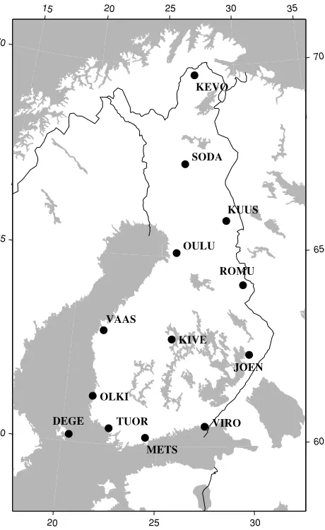
We used 6months (184 days) of data fromthe Finnish permanent GPS network, FinnRef. The network consists of 13 stations between the latitudes 60◦N and 70◦N, with calculated vector lengths varying from 110 to 1100 km
(Fig. 1). The time period 1 May–31 October 2006 was chosen in order to exclude observations recorded while the antennamay have been covered by snow, because snow can distort solutionsmarkedly (Poutanenet al., 2005).
4.
GPS Proce
ss
ing
We used the GPS processing software Bernese v. 5.0 (Dach et al., 2007) to calculate daily station coordinates with the ionosphere-free L3 combination in double dif-ference mode. We formed a total of 12 vectors radially from METS (Fig. 1). The coordinates of METS were kept fixed to ITRF2000 (International Terrestrial Reference Frame; Boucher et al., 2004) (epoch 2005.7). The ele-vation cut-off angle was 5◦, and an elevation-dependent weighting using cos2(z) was adopted. Station-specific ocean load tables were also employed (Bos and Scherneck, http://www.oso.chalmers.se/˜loading/). All of the time se-ries were calculated in the same way, except for the tropo-sphere handling. There were 15 different processing op-tions, summarised in Table 1.
In GPS processing, the total troposphere correction is the sumof two parts: the hydrostatic part, which is taken from
ana priorimodel, and a wet part, which is estimated in the
15
20
20
25 25
30
30 35
60
60 65
65 70
70
KIVE ROMU
OLKI
OULU
METS
JOEN SODA
TUOR VIRO
VAAS
KUUS KEVO
DEGE
Fig. 1. The FinnRef network of permanent GPS stations.
processing. In our computations, we use this approach in three processing schemes. First, we used the Niellmapping function, i.e. Saastamoinen zenith delays and Niell m ap-ping function as provided by the Bernese software without anymodifications (SN). Secondly, we derived (hydrostatic or total) zenith delays froman NWM, subsequently using these as an input together with the Niell mapping func-tion (HN and EN). Another way of correcting the tropo-sphere is to derive the total slant delays. We derived these total slant delays froman NWM, removing themdirectly fromthe observations (modified RINEX files) and process-ing data without any troposphere estimation (HS). This pro-cessing scheme is explained inmore detail in Nordmanet al.(2007). The EV solution was implemented in the same way as the HS, i.e. with RINEXmanipulation.
Table 1. Different troposphere handling schemes. The code for each scheme is an abbreviation. The first letter signifies the troposphere
model (S=Saastamoinen, H=HIRLAM and E=ECMWF; Tro-pospheremodel column), and the second letter indicates themapping function (N=NMF, S=slant delay and V=VMF1; MF-column). The last two numbers indicate whether site-specific parameters and gra-dients were used or not (0=not used, 1=used).
Abbreviation Tropospheremodel MF Site-specific Gradients
SN00 Saastamoinen Niell no no
SN10 Saastamoinen Niell yes no
SN11 Saastamoinen Niell yes yes
HN00 HIRLAM Niell no no
HN10 HIRLAM dry Niell yes no
HN11 HIRLAM dry Niell yes yes
EN00 ECMWF Niell no no
EN10 ECMWF dry Niell yes no
EN11 ECMWF dry Niell yes yes
HS00 HIRLAM Slant no no
a parameter spacing of 2 h. Horizontal gradient estimation is a common way of coping with the azimuthal asymmetry of the local troposphere. The gradients are estimated once every 24 h.
4.1 RINEX manipulation test
We tested our RINEX manipulation scheme using the Saastamoinen model. Saastamoinen is a troposphere re-fractivitymodel based on the laws associated with ideal gas (Saastamoinen, 1973). We calculated slant delays using
ρ= 0.002277 which is the formula (11.11) in the Bernesemanual (Dach
et al., 2007). ρ is the troposphere slant delay; z is the satellite’s zenith distance;p,eandT atmospheric pressure, partial water vapour pressure and temperature, respectively.
B andδR are correction terms of which the former is de-pendent on the station height and the latter is not yet im
ple-mented in Bernese. We then corrected the RINEX files with the computed slant delays.
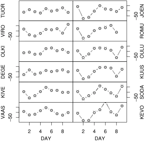
We calculated two 9-day time series using the same data. The first time series was produced using the manipulated RINEX and the second with original, un-manipulated files together with the Saastamoinenmodel within Bernese—in both cases without any site-specific parameters. The result for the up component of all the stations can be seen in Fig. 2. The crosses were calculated using the Saastamoinenmodel enabled in Bernese, and the circles were calculated with the
manipulated files. Typically, the up component is the one to show the greatest variance and discrepancies in the time series. One of the reasons for this is that the troposphere zenith delays are highly correlated with the up component due to the observation geometry.
As Fig. 2 shows, the differences between the up time series are small; for the horizontal components, the dif-ferences are even smaller. The standard deviations for
TUO
Fig. 2. The up component of 12 stations for 9 days. The crosses are the data computed with Saastamoinen within Bernese, and the circles are themanipulated data solutions. The scale is inmillimetres.
the stations are 1–17mm, 2–7mmand 17–64mm in the north, east and up component, respectively, for the
un-manipulated files, and 1–15mm, 2–8 mmand 17–60mm
for the same components using themanipulated files. The differences are not statistically significant even at an 80% confidence level. Another measure for the goodness of the solution is the root-mean-square (RMS) of the residu-als. This test shows that themanipulated files have a two-to threefold larger RMS than the un-manipulated files, al-though the same Saastamoinen model is used in both and no site-specific parameters or gradients are estimated in ei-ther. The RMS also seems to be dependent on the baseline length when using themanipulated data, but the reason for this is unknown. Since the standard deviations of them a-nipulated and un-manipulated data are alike, we choose to use the standard deviation (repeatability) of the time series for the comparisons in the next section.
5.
Re
s
ult
s
The GPS processing produced 15 different time series for all of the stations and for all three components. Five single values with the largest difference to themean were removed as outliers, and the standard deviation for each processing scheme, station and component was then calculated. The standard deviation represents the repeatability of the so-lution. A one-sided F-test (e.g. Brandt, 1999) with 99% confidence level was used to compare the statistical signifi-cance of the differences between processing schemes.
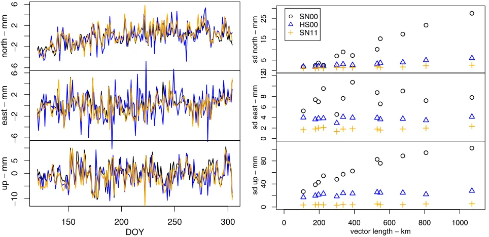
re-150 200 250 300 DOY
Fig. 3. Example fromOulu of the time series of all three components. The solid black line is SN11, the grey line (blue) HS10 and the dotted black line (orange) EV11. Note that the range for the horizontal component is 12mmand for the vertical component, 24mm.
sult indicates that the gradients estimated during the GPS processing performbetter than gradient estimation fromthe HIRLAMmodel. The HS10 of OULU was slightlymore scattered in the east component than the others, whichmay be explained by the position of the OULU station near the coast of the Baltic Sea. The coast extends in a north-south direction, which leads to a permanent azimuthal inhom o-geneity in the troposphere—the land–sea difference. Only if the gradients are estimated is the east-west inhomogeneity for OULU considered; otherwise they are not, and the east component time series ismore scattered. However, none of the other coastal GPS stations had the same behaviour. The other time series for OULU have the same characteristics; only the ranges vary, depending on the solution. The SN00 has a range of 60mmin the north component, whereas the HS00 has a range of 20mm.
The standard deviations of three time series for all the sta-tions are depicted in Fig. 4. The SN00 solution (circles) has the greatest scatter in all three components. When NWM-based troposphere delays are used, the scatter reduces
re-markably (HS00, triangles), and the baseline length depen-dence of the standard deviation is also reduced. The SN11 (plus signs) shows the behaviour of a less-scattered time series. As Table 2(b, c) shows, all of the time series us-ing additional parameter estimation are in the same order of
magnitude. The scatter of the vector component is depen-dent on the azimuth of the baseline. Due to the geometry of our GPS network, the vectors of this study aremostly ori-ented in the north-south direction, which explains the length dependence of the north component.
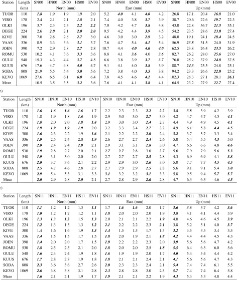
Table 2(a) presents the standard deviations for all of the stations and all of the components for the 00-processing schemes, i.e. schemes with no additional parameter estim a-tion. The last line shows themean value of each column.
Fig. 4. The standard deviation of all the stations and processing schemes SN00, HS00 and SN11 for all three components, north, east and up (in
mm). Note that the scale for each component is different.
The HS00 scheme gives the lowest standard deviation in
most cases, as expected, because it is the scheme that both uses themost accurate tropospheremodel and accounts for the azimuthal asymmetry. It can be also seen that all of the schemes are affected by vector length, although SN00 is the
most extreme example. All of the reductions fromSN00 to any other processing scheme are statistically significant, ex-cept for the north component of TUOR and VIRO.
Table 2(b) presents the results for 10-processing schemes, as processed with site-specific parameter estim a-tion. No specific conclusions can be drawn; for the north component, SN10 gives the lowest standard deviation, but for the east component HS10 is better. One reason for dis-crepancy is that in Finland the weather fronts often propa-gate in an easterly or northeasterly direction. In this case, the solution with gradients, HS10, gives the best results. For the up component, EV10 is the best, but HS10 is also quite good. It is worth noting that the differences between different schemes are small—tenths ofmillimetres inmost cases—and thus not statistically significant.
Table 2(c) presents the standard deviations for the 11-processing schemes, i.e. with both site-specific parameters and gradient estimation. Standard Bernese processing us-ing both the site-specific parameter and gradient estimation (SN11) yields the best results for all three components. As for the 10-processing schemes in Table 2(b), none of the differences are statistically significant. The HS11 does not have a single low value. Thismight be due to the fact that azimuthal differences are already included in the slant de-lay derivation and, therefore, the gradient estimation does not increase the accuracy.
reduc-Table 2. (a) Standard deviations inmillimetres for the 00-processing schemes. The abbreviations are explained in Table 1. The lowest (best) standard deviation values are in bold and italics for each station and component, respectively. The last line is themean value of all the stations. (b) Same as Table 2(a), results for 10-schemes. (c) Same as Table 2(a), results for 11-schemes.
(a)
Station Length SN00 HN00 EN00 HS00 EV00 SN00 HN00 EN00 HS00 EV00 SN00 HN00 EN00 HS00 EV00
(km) North (mm) East (mm) Up (mm)
TUOR 110 1.8 1.9 1.9 1.9 2.0 5.2 4.0 4.1 4.0 4.2 26.8 17.1 20.4 16.8 21.0
VIRO 178 2.4 2.1 2.1 1.8 2.1 7.4 4.0 3.8 3.7 3.9 38.7 20.6 22.6 19.7 22.3
OLKI 196 3.7 2.3 2.3 2.2 2.2 7.0 4.2 4.7 3.8 4.8 43.0 22.8 36.7 21.5 35.1
DEGE 224 2.6 2.0 2.1 2.0 2.0 9.5 4.2 4.4 3.9 4.5 54.2 23.5 28.6 23.0 27.4
KIVE 300 7.0 2.8 2.8 2.7 3.0 4.6 3.0 3.0 2.9 3.2 48.0 19.1 24.1 18.4 24.5
VAAS 336 8.9 3.3 3.6 3.1 3.7 7.6 4.7 5.4 4.1 5.4 56.9 23.8 31.5 24.0 31.9
JOEN 390 7.2 2.9 2.8 2.7 2.8 10.7 4.4 4.0 4.0 4.0 62.5 23.8 26.4 23.5 26.2
ROMU 530 10.2 4.1 3.6 3.3 3.6 8.8 4.1 3.6 4.0 3.6 82.7 26.2 28.0 25.6 27.0
OULU 548 15.3 4.3 4.4 3.7 4.5 6.6 3.8 3.9 3.7 3.7 76.0 25.2 37.9 24.8 37.5
KUUS 676 17.6 4.7 4.8 4.0 4.7 9.1 4.1 4.0 3.8 3.9 88.7 24.3 25.5 24.8 25.1
SODA 808 21.9 5.5 5.4 5.0 5.6 7.2 3.8 4.0 3.5 3.8 94.2 23.3 26.6 22.0 25.2
KEVO 1069 27.6 6.5 6.1 6.0 6.4 7.8 4.5 4.6 4.1 4.4 102.3 28.3 27.1 28.1 26.1
Mean 10.5 3.5 3.5 3.2 3.6 7.6 4.1 4.1 3.8 4.1 64.5 23.2 27.9 22.7 27.4
(b)
Station Length SN10 HN10 EN10 HS10 EV10 SN10 HN10 EN10 HS10 EV10 SN10 HN10 EN10 HS10 EV10
(km) North (mm) East (mm) Up (mm)
TUOR 110 1.6 1.6 1.6 1.6 1.7 2.2 2.3 2.3 2.2 2.2 3.8 3.8 3.9 4.2 3.9
VIRO 178 1.8 1.9 1.8 1.6 1.9 2.9 3.0 3.0 2.7 3.0 4.2 4.7 4.7 4.5 4.1
OLKI 196 1.8 2.0 2.0 1.8 1.8 2.9 3.0 3.0 2.4 2.7 4.4 4.9 4.9 4.5 4.1
DEGE 224 1.9 1.9 1.9 1.9 2.0 3.2 3.3 3.4 2.7 3.2 4.9 6.1 5.8 4.4 4.5
KIVE 300 1.6 2.3 2.2 1.9 1.6 2.1 2.2 2.2 2.0 2.4 3.2 3.7 3.7 3.3 3.4
VAAS 336 1.9 2.5 2.4 2.0 1.9 2.6 2.7 2.7 2.4 2.6 5.0 5.4 5.5 4.3 5.0
JOEN 390 2.0 2.4 2.4 2.0 2.1 2.9 3.1 3.1 2.8 3.0 4.7 6.6 6.6 4.8 4.6
ROMU 530 1.9 2.8 2.7 2.0 2.1 2.7 2.7 2.8 3.0 2.7 5.6 7.9 7.9 5.6 5.3
OULU 548 1.9 3.1 3.0 2.0 2.0 2.7 2.7 2.7 2.5 2.8 4.3 6.9 6.9 4.1 3.8
KUUS 676 2.0 3.7 3.6 2.1 2.2 2.9 2.9 3.0 2.6 3.0 5.0 7.7 7.7 4.5 4.5
SODA 808 2.5 4.7 4.6 2.8 2.7 2.7 2.9 2.9 2.5 2.8 5.6 9.1 9.1 5.4 5.0
KEVO 1069 2.9 5.4 5.3 3.1 3.3 3.1 3.2 3.2 3.1 3.3 5.8 9.5 9.4 5.7 5.7
Mean 2.0 2.9 2.8 2.0 2.1 2.7 2.8 2.9 2.6 2.8 4.7 6.3 6.3 4.6 4.5
(c)
Station Length SN11 HN11 EN11 HS11 EV11 SN11 HN11 EN11 HS11 EV11 SN11 HN11 EN11 HS11 EV11
(km) North (mm) East (mm) Up (mm)
TUOR 110 1.1 1.2 1.2 1.3 1.1 1.7 1.6 1.6 2.0 1.7 3.6 3.6 3.7 4.2 3.6
VIRO 178 1.0 1.2 1.2 1.2 1.1 1.8 2.0 2.0 2.0 1.9 3.8 4.1 4.1 4.4 3.9
OLKI 196 1.3 1.3 1.3 1.5 1.3 2.0 2.1 2.1 2.2 1.9 4.0 4.6 4.6 4.5 3.9
DEGE 224 1.2 1.3 1.3 1.3 1.2 2.1 2.2 2.2 2.3 2.1 3.8 5.2 5.1 4.0 3.7
KIVE 300 1.4 1.6 1.6 1.9 1.3 1.4 1.5 1.5 1.7 1.5 3.2 3.5 3.5 3.4 3.5
VAAS 336 1.4 1.5 1.5 1.7 1.5 1.8 2.0 1.9 2.1 1.8 4.2 4.4 4.4 4.5 4.3
JOEN 390 1.4 2.0 2.0 1.7 1.5 1.9 2.2 2.2 2.3 2.0 3.9 5.6 5.6 4.7 4.2
ROMU 530 1.8 2.5 2.5 2.1 2.0 1.8 2.0 2.0 2.5 1.8 5.5 6.4 6.5 6.0 5.6
OULU 548 1.6 2.4 2.4 1.9 1.8 1.6 1.9 1.9 2.0 1.7 4.0 5.4 5.4 4.4 4.2
KUUS 676 1.7 2.8 2.8 1.9 1.8 1.8 2.1 2.1 2.4 2.1 4.1 5.6 5.6 4.7 4.3
SODA 808 2.3 3.6 3.6 2.7 2.6 2.0 2.3 2.3 2.4 2.1 5.4 7.4 7.4 6.1 5.5
KEVO 1069 2.6 3.8 3.8 3.1 2.8 2.3 2.8 2.8 3.0 2.5 5.7 7.4 7.4 6.4 5.8
Mean 1.6 2.1 2.1 1.9 1.7 1.9 2.1 2.1 2.2 1.9 4.3 5.3 5.3 4.8 4.4
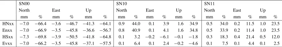
tion or increase has been computed with respect to the SN-solution for all the components. Reductions in standard deviation have been denoted with a negative sign (scatter decreases), and increases in standard deviation aremarked with a plus sign (scatter increases). Comparing SN with itself yields 0.0%.
In the 00-solutions the decrease in the standard
per-Table 3. Comparison of different processing techniques for all the stations. Numbers show the reduction (negative values) or increase (positive values) in standard deviation inmillimetres (mm) and in percentages (%), compared with the SN-solution.
SN00 SN10 SN11
North East Up North East Up North East Up
mm % mm % mm % mm % mm % mm % mm % mm % mm %
HNxx −7.0 −66.4 −3.6 −46.7 −41.3 −64.1 0.9 44.0 0.1 3.9 1.6 34.9 0.5 34.0 0.2 11.5 1.0 23.5 Enxx −7.0 −66.9 −3.5 −45.8 −36.6 −56.7 0.8 40.9 0.1 4.1 1.6 34.8 0.5 33.9 0.2 11.4 1.0 23.5 HSxx −7.3 −69.8 −3.9 −50.5 −41.8 −64.8 0.1 3.2 −0.2 −6.1 −0.1 −1.8 0.3 18.3 0.4 21.4 0.5 12.0 Evxx −7.0 −66.2 −3.5 −45.8 −37.1 −57.5 0.1 6.4 0.1 2.4 −0.2 −4.6 0.1 7.5 0.1 4.4 0.1 2.5
forms better in the up component, most likely due to the higher resolution of HIRLAM. The EV00 solution yields basically the same reductions as EN00, indicating that there is no great difference between the NMF and VMF1 in this resolution. Looking at HN00 and HS00 reductions, it can be concluded that the better zenith delaymodel has the great-est effect. However, the slant delay approach provides the highest precision.
For the 10-schemes, the SN10 seems to be the best op-tion. None of the other schemes yield statistically signif-icant improvements. The next-best solution is the HS10, which does notmake the solutionmuch better or worse. The HN10 and EN10, which were calculated using thea priori
hydrostatic zenith delays, degrade all the components. In the third case, in which both site-specific parameters and horizontal gradients are estimated, the SN11 is themost reliable solution. The next best solution is the EV11, which can be explained by the gradients in the HS slant delays, as discussed above.
6.
Di
s
cu
ss
ion
The simulation of non-scientific software shows that us-ingmore precise tropospheremodels reduces the standard deviation of all the components in the GPS time series. In cases where no additional parameters are estimated, the re-duction can be up to 60% compared with the standard solu-tion. The reduction also depends on the length of the vector. There are no great differences between different processing schemes when site-specific parameters and/or gradients are estimated. Standard deviations show a statistically signifi-cant reduction only at some stations and components.
The discrepancies we see can be partly due to loading ef-fects that influence all of the GPS stations. The time series, therefore, contain not only observational noise, but also the geophysical loading effects of the atmosphere, hydrology and non-tidal variations of the sea. When troposphere pa-rameters (zenith delays and gradients) and station height are estimated in one adjustment, the parameters are corre-lated, indicating that a part of the real variation by loading can be compensated by the troposphere parameter estim a-tion, as was discussed in Analysis section. Thismeans that a smaller repeatability (i.e. standard deviation) of station height does not necessarilymean that the tropospheric re-fraction is handled in a better way. Thismight be one of the reasons why SN10 and SN11 give such good results.
Other studies have shown improvements whenmore so-phisticated mapping functions are used. However, these studies differ fromthe present study in terms of processing
windows, strategies, baseline lengths, etc. We are also us-ing a regional network, where the troposphere is quite sim -ilar for all the stations. In their study, Tesmeret al.(2007) found an improvement of 3, 3.5 and 7% for the north, east and up components, respectively, when they switched from
the NMF to the VMF1 in their VLBI analysis. We see no such distinctive reductions in our results, but our network is not global. Bocket al.(2002) declared a repeatability of 5– 10mmwith a 1-h processing window for the vertical com -ponent. Mapping function studies indicate a 50% reduction in scatter when more sophisticated mapping functions are used (MacMillan and Ma, 1998; Niell, 2001), which is the same order ofmagnitude we found for our non-site-specific parameter case (00).
We used the GPS in double differencemode, where the coordinates of the other end of the vector are kept fixed. The troposphere is estimated for both ends of the vector. How-ever, it is not known how a possible error in troposphere estimation will affect the final coordinates. The effect of the troposphere could be seen more clearly in PPP (Pre-cise Point Positioning) solutions. A recent study using slant delays and PPP-processing shows improved repeatabilities when ray-traced data are used together with residual tro-posphere estimation, as compared with standard process-ing (Hobigeret al., 2008). The improvement achieved by the residual troposphere estimation in their study is in the same order ofmagnitude as that observed when we com -pared the HS00 and HS10 results here, yielding a couple of
millimetres in standard deviation for horizontal components and 15–20mmfor the vertical.
7.
Conclu
s
ion
s
We have considered the effect of different troposphere estimation techniques on GPS processing, using Bernese v. 5.0 and employing 6months of data for 13 permanent GPS stations. Five different troposphere model and mapping function combinations were used for the purposes of com -parison: themapping functions NMF and VMF1, the ray-tracing-based slant delay model, and, finally, two NWM-derived troposphere zenith delays used with the Niellm ap-ping function.
The ray-tracing-based troposphere slant delays were im -plemented in GPS processing through RINEX filem anip-ulation at the observation level. The advantage of this
method is that it is independent of processing software and is also applicable to other error sources, such as ionosphere delay or loading.
estimated, the standard deviation of the GPS time series is reduced by 60% in all three components when NWM-based tropospheric delays are introduced. In this case, the slant delays derived by ray tracing yielded the best results. The improved troposphere handling also reduces the base-line length dependence of the standard deviation. However, the results do show further improvements when site-specific troposphere parameters and gradients are estimated, indi-cating that the numerical weathermodels are not at an accu-racy level thatmakes site-specific residual troposphere
esti-mation unnecessary.
When site-specific parameters or both site-specific pa-rameters and horizontal gradients are estimated, there are no statistically significant differences in the different process-ing schemes. The standard Bernese processing yields the lowest standard deviations. The results show that ana pri-orireduction of observations bymodelled slant troposphere delays gives comparable results to the estimation of tropo-sphere zenith delay and is therefore an appropriatemethod. Estimating the site-specific troposphere parameters and hor-izontal gradients is stillmandatory when the highest accu-racy in double difference GPS processing is required.
Acknowledgments. This work was partly funded by the Finnish Funding Agency for Technology and Innovation (TEKES), deci-sion number 40415/04 and by the Finnish Academy of Science, decision number 117094.
References
Bock, O., J. Tarniewicz, Ch. Thom, and J. Pelon, The effect of inhom o-geneities in the lower atmosphere on coordinates determined fromGPS
measurements,Phys. Chem. Earth,27, 323–328, 2002.
Boehm, J. and H. Schuh, Viennamapping functions in VLBI analyses,
Geophys. Res. Lett.,31, L01603, doi:10.1029/2003GL018984, 2004. Boehm, J., B. Werl, and H. Schuh, Tropospheremapping functions for
GPS and very long baseline interferometry fromEuropean Centre for Medium-Range Weather Forecasts operational analysis data,J. Geo-phys. Res.,111, B02406, doi:10.1029/2005JB003629, 2006a. Boehm, J., A. Niell, P. Tregoning, and H. Schuh, Global Mapping
Func-tion (GMF): A new empiricalmapping function based on num er-ical weather model data, Geophys. Res. Lett., 33, L07304, doi:10. 1029/2005GL025546, 2006b.
Boucher, C., Z. Altamimi, P. Sillard, and M. Feissel-Vernier, The ITRF2000 (IERS Technical Note; 31) Frankfurt am Main: Verlag des Bundesamts f¨ur Kartographie und Geod¨asie, 289 pp., 2004.
Brandt, S.,Data analysis, Statistical and computational methods for sci-entists and engineers, Springer-Verlag, 1999.
Dach, R., U. Hugentobler, P. Fridez, and M. Meindl (Eds.),Bernese GPS Software, Version 5.0, 612 pp., Astronomical Institute, University of Berne, 2007.
Elgered, G., H.-P. Plag, H. van der Marel, S. Barlag, and J. Nash (Eds.),COST Action 716—Exploitation of ground-based GPS for opera-tional numerical weather prediction and climate applications, European Union, Rep. EUR 21639, COST Office, Brussels, Belgium, 234 pp., 2005.
Eresmaa, R. and H. J¨arvinen, An observation operator for ground-based GPS slant delays,Tellus,58A, 131–140, 2006.
Eresmaa, R., H. J¨arvinen, M. Nordman, M. Poutanen, J. Syrj¨arinne, and J.-P. Luntama, Parameterization of tropospheric delay correction form o-bile GNSS positioning: a case study of a cold front passage,Meteorol.
Applic., 2008 (submitted).
Hobiger, T., R. Ichikawa, T. Takasu, Y. Koyama, and T. Kondo, Ray-traced troposphere slant delays for precise point positioning,Earth Planets Space,60, e1–e4, 2008.
Kr¨ugel, M., D. Thaller, V. Tesmer, M. Rothacher, D. Angermann, and R. Schmid, Tropospheric parameters: combination studies based on homogeneous VLBI and GPS data, J. Geod., 81, 515–527, doi:10. 1007/s00190-006-0127-8, 2007.
MacMillan, D. S. and C. Ma, Usingmeteorological data assimilationm od-els in computing tropospheric delays atmicrowave frequencies,Phys. Chem. Earth,23, 97–102, 1998.
Niell, A. E., Globalmapping functions for the atmosphere delay at radio wavelengths,J. Geophys. Res.,101(B2), 3227–3246, 1996.
Niell, A. E., Preliminary evaluation of atmosphericmapping functions based on numerical weathermodels,Phys. Chem. Earth,26, 475–480, 2001.
Niell, A. E., A. J. Coster, F. S. Solheim, V. B. Mendes, P. C. Toor, R. B. Langley, and C. A. Upham, Comparison ofmeasurements of
at-mospheric wet delay by radiosonde, water vapor radiometer, GPS, and VLBI,J. Atmos. Oceanic Technol.,18, 830–850, 2001.
Nordman, M., R. Eresmaa, M. Poutanen, H. J¨arvinen, H. Koivula, and J.-P. Luntama, Using numerical weather predictionmodel derived tropo-spheric slant delays in GPS processing: a case study,Geophys.,43(1–2), 43–51, 2007.
Poutanen, M., J. Jokela, M. Ollikainen, H. Koivula, M. Bilker, and H. Virtanen, Scale variation of GPS time series, inA Window on the Future of Geodesy, IAG General Assembly in Sapporo, Japan 2003, edited by F. Sans`o, 15–20, IAG Symposia 128, Springer-Verlag, 2005.
Saastamoinen, J., Contributions to the theory of atmospheric refraction,
Bull. G´eod´esique,107, 13–34, 1973.
Simmons, A. J. and J. K. Gibson (Eds.),The 40 Project Plan, ERA-40 Proj. Rep. Ser. 1, Eur. Cent. for Medium-Range Weather Forecasts, Reading, U.K., 2000.
Snajdrova, K., J. Boehm, P. Willis, R. Haas, and H. Schuh, Multi-technique comparison of tropospheric zenith delays derived during the CONT02 campaign,J. Geod.,79, 613–623, doi:10.1007/s00190-005-0010-z, 2006.
Stoyanov, B., R. Haas, and L. Gradinarsky, Calculatingmapping functions from the HIRLAM numerical weather predictionmodel, in Interna-tional VLBI Service for Geodesy and Astrometry 2004 General Meeting Proceedings, edited by N. R. Vandenberg and K. D. Baver, 471–475, NASA/CP-2004-212255, 2004.
Tesmer, V., J. Boehm, R. Heinkelmann, and H. Schuh, Effect of different troposphericmapping functions on the TRF, CRF and position tim e-series estimated fromVLBI,J. Geod., doi:10.1007/s00190-006-0126-9, 2007.
Tregoning, P. and T. van Dam, Atmospheric pressure loading corrections applied to GPS data at the observation level,Geophys. Res. Lett.,32, L22310, doi:10.1029/2005GL024104, 2005.
Troller, M., A. Geiger, E. Brockmann, and H.-G. Kahle, Determination of the spatial and temporal variation of tropospheric water vapour using CGPS networks,Geophys. J. Int.,167, 509–520, doi:10.1111/j.1365-246X.2006.03101.x, 2006.
Und´en, P., L. Rontu, H. J¨arvinen, P. Lynch, J. Calvo, G. Cats, J. Cuxart, K. Eerola, C. Fortelius, J. A. Garcia-Moya, C. Jones, G. Lenderlink, A. McDonald, R. McGrath, B. Navascu´es, N. Woetman Nielsen, V. Ødegaard, E. Rodriguez, M. Rummukainen, R. R˜o˜om, K. Sattler, B. Hansen Sass, H. Savij¨arvi, B. Wichers Schreur, R. Sigg, H. The, and A. Tijm,HIRLAM-5 Scientific Documentation, Available from Hirlam-5 Project, c/o Per Und´en, SMHI, S-60176, Norrk¨oping, Sweden, 144 pp., 2002.