DOI: 10.1534/genetics.106.069955
Quantifying Evidence for Candidate Gene Polymorphisms: Bayesian
Analysis Combining Sequence-Specific and Quantitative Trait
Loci Colocation Information
Roderick D. Ball
1Scion (New Zealand Forest Research Institute Limited), Rotorua, New Zealand Manuscript received December 18, 2006
Accepted for publication October 15, 2007
ABSTRACT
We calculate posterior probabilities for candidate genes as a function of genomic location. Posterior probabilities for quantitative trait loci (QTL) presence in a small interval are calculated using a Bayesian model-selection approach based on the Bayesian information criterion (BIC) and used to combine QTL colocation information with sequence-specific evidence, e.g., from differential expression and/or asso-ciation studies. Our method takes into account uncertainty in estimation of number and locations of QTL and estimated map position. Posterior probabilities for QTL presence were calculated for simulated data withn¼100, 300, and 1200 QTL progeny and compared with interval mapping and composite-interval mapping. Candidate genes that mapped to QTL regions had substantially larger posterior probabilities. Among candidates with a given Bayes factor, those that map near a QTL are more promising for further investigation with association studies and functional testing or for use in marker-aided selection. The BIC is shown to correspond very closely to Bayes factors for linear models with a nearly noninformative Zellner prior for the simulated QTL data withn$100. It is shown how to modify the BIC to use a subjective prior for the QTL effects.
A
quantitative trait locus (QTL) is a location or small region in the genome associated with variation in a quantitative (i.e., continuously variable) trait. QTL are mapped by statistical analysis of marker–trait associa-tions within a QTL mapping family or pedigree. The ac-curacy of QTL-mapping location estimates is typically of the order of tens of centimorgans, considerably narrow-ing down the location of possible functional loci, but not enough for brute force sequencing to locate genes. Hence there is the need to combine QTL mapping with other evidence. In this article we combine evidence for candidate polymorphisms with QTL-mapping data, using the posterior probabilities for the candidate polymor-phisms as priors for the QTL analysis.Evidence for candidate polymorphisms can be obtained from various sources:e.g., from assays of differential ex-pression between tissue types or between genotypes using microarrays, from homology with genes in other species where there is evidence for effects on the corresponding trait, from genes mapping to a QTL region in another species, from polymorphisms in genes coding for pro-teins in a biosynthetic pathway, from an association study, or from a combination of these sources.
Quantifying the evidence from all of these possible sources would be a large undertaking, with many
evalua-tions particular to specific cases. To limit the scope of this article we assume candidate genes are given, and the evidence is quantified in the form of posterior proba-bilities and/or Bayes factors. Candidates could also be selected using QTL data (e.g., in a genome-scan ap-proach), in which case the method of this article would
not apply unless further independent QTL data were available to assess the QTL colocation.
Information from these sources often represents only weak or moderately strong evidence;e.g.,4000 candi-date polymorphisms were differentially expressed for wood density (S. Cato, personal communication). Since prior
odds for a random candidate gene are low (e.g., 1/3000 if there are 30,000 genes and 10 affecting the trait), fur-ther evidence is needed to justify the expense of func-tional testing, and to most effectively select candidates for testing, or for marker-aided selection applications.
In this article we quantify the additional evidence for a candidate gene from QTL colocation: this is based on the estimated map location of the candidate and QTL regions identified using independent data from a QTL-mapping pedigree. Our approach requires Bayesian posterior probabilities for a QTL to be present in a small genomic interval. To motivate the approach we first dis-cuss possible alternative QTL-mapping approaches, both Bayesian and non-Bayesian.
Non-Bayesian QTL mapping:A candidate gene is of-ten considered to colocate with a QTL if the estimated candidate gene locus falls within a 95% confidence 1Address for correspondence:Scion (New Zealand Forest Research Institute
Limited), 49 Sala St., P.B. 3020, Rotorua, New Zealand. E-mail: [email protected]
interval for QTL location. Various methods have been used to estimate confidence intervals for QTL location: the region around a peak where the interval-mapping LOD score (Landerand Botstein1989) drops by less
than a certain number, a method based on the sampling variation in estimated QTL location under bootstrap resampling (Visscheret al.1996), and a method using
the empirical formula of Darvasiand Soller(1997).
All of these methods have shortcomings. What LOD drop-off to use in a given situation is not clear and the graph of LOD scores may not even be unimodal due to artificial peaks in the likelihood ratio between markers. Bootstrap methods have been reported as giving differ-ent answers and inexact confidence-interval coverage (Bennewitz et al. 2002). Manichaikul et al. (2006)
found that, when marker density is not high, bootstrap confidence intervals based on maximum-likelihood esti-mates of QTL location can be unstable due to the strong tendency of the maximum-likelihood estimate to occur at a marker, while Bayesian credible intervals exhibited stable coverage on the same simulated data. The Darvasi
and Soller(1997) estimate (Equation 42 below) is based
on the size of QTL effects. Unless power is high to detect the true size of effect, selection bias and sampling error in estimates of QTL effects will result in large errors in confidence-interval widths.
A more fundamental limitation of all the confidence-interval methods is that they condition on the existence of a single QTL in a region. For example, the interval-mapping LOD score is, up to an unknown constant, approximately the log-posterior distribution of QTL locationassumingexistence of asingleQTL in a region (Senand Churchill2001); hence it cannot be used to
infer the number of QTL. As we shall see, results can be misleading if there are two QTL when one is assumed or vice versa.
To limit the scope of this article we compare only the Darvasi and Soller confidence intervals with posterior probabilities from Bayesian model selection.
Bayesian QTL mapping: The main advantage of the Bayesian approach in this context is that the required probabilities can be obtained directly, using a Bayesian model selection approach, where multiple models are considered according to their probabilities. In Bayesian model selection approaches (reviewed by Sillanpa¨ a¨and
Corander2002), inference is based on the total
pos-terior probability of models satisfying a given property, and estimation is based on model averaging, averaging over estimates of effects from each model, weighted ac-cording to the posterior probability for models. Ball
(2001) used a Bayesian model selection approach for QTL mapping where each model is a linear regression model for the trait as a function of a fixed set of markers, and approximate posterior probabilities for models were calculated using a modified Bayesian information crite-rion (BIC) (previously used by Broman1997 and Broman
and Speed2002 to select a single model).
This approach can be used to infer the genetic ar-chitecture: for example, the posterior probability that there are two QTL on a chromosome is the sum of probabilities for models with two selected markers on that chromosome (Ball2001; Yandellet al.2002).
In-teractions (dominance and epistasis) can be allowed for simply by specifying the appropriate prior probabilities for interaction terms (Ball2001; Bogdanet al.2004).
The BIC is easily and rapidly calculated from standard regression model statistics, but is based on an asymp-totic approximation. Alternatives include MCMC meth-ods and analytical calculations. Posterior probabilities for individual models can be obtained in closed form if the Zellner priors are used (Smithand Kohn1996; Sen
and Churchill 2001). In fact, using the BIC is
ap-proximately equivalent to using the Bayes factors cal-culated using the Zellner prior with prior information equivalent to a single sample point½c¼nin (18) below. Hence closed-form calculations can be used as a check on the accuracy of the BIC approximation.
Interval mapping and composite-interval mapping likelihood-ratio statistics are for comparing a model with a single QTLvs.the null model, corresponding to a null hypotheses of no QTL anywhere. These methods test for the presence of a linked QTLbut we need a test for a QTL at a specific location. To quantify the evidence for a polymorphism at locus x, we define a Bayes factor,
BQ(x), as the limiting case of the Bayes factor for testing
the hypothesis of a QTL in a small interval (x,x1dx)vs.
no QTLin the small interval. The possibility of QTL at other locations, possibly on the same chromosome, is allowed for in our null hypothesis. The Bayes factor,
BQ(x), is combined with prior probability and Bayes
factor for a candidate gene to obtain an expression for the posterior probability for a candidate polymorphism atxto be functional. The posterior probability is then integrated overx to incorporate uncertainty in map position.
The rest of this article is structured as follows. The
methodssection contains five parts: (1) showing how to
incorporate QTL colocation given posterior probabilities for QTL presence, (2) computing posterior probabilities for QTL presence using the Bayesian model-selection approach from Ball(2001), (3) introducing the Zellner
priors and describing how closed-form calculations with these priors can be used to check on the accuracy of the BIC, (4) describing the data simulation, and (5) show-ing how to incorporate subjective prior information on the sizes of QTL effects into the BIC. In the results
METHODS
Incorporating QTL colocation information:It follows from Bayes’ theorem that the prior odds for a hypothesis are multiplied by the Bayes factor to give the posterior odds. Without QTL colocation information the poste-rior odds for a candidate gene are:
pc
1pc
¼Bc3
pc
1pc; ð1Þ
wherepc¼Pr(H1jyc) is the posterior probability for the
candidate to represent a functional trait locus, andBcis
the Bayes factor representing the strength of evidence forH1overH0in the data for the candidate gene,
de-noted byyc.
Now suppose we have independent data, denoted byyq,
from a QTL mapping pedigree. It follows easily from Bayes’ theorem that, when analyzing multiple independent data sets, the posterior for the first data set can be used as the prior for the second data set, giving the same posterior as if the combined data were analyzed jointly. Thus we can use the posterior from the candidate gene data,yc, as prior
information for the analysis of the QTL data,yq.
Note that, almost by definition, a candidate poly-morphism at locationxis a functional locus if, and only if, there is a QTL atx.
To combine candidate gene and QTL colocation evidence, we first consider the posterior for QTL in a small interval,I, in the absence of candidate gene in-formation, then by comparing prior and posterior prob-abilities obtain the strength of evidenceBQ(I) for a QTL
inI, and then combine this with evidence from the can-didate gene data, giving posterior probabilities ofH1for
any givenIcontaining the candidate. LetpQ(x) be defined by
pQðxÞ ¼ lim
dx/0Prð
dQ:Qis a QTL andQ 2 ðx;x1dxÞÞ=dx; ð2Þ where probabilities are posterior probabilities givenyq.
LetpQ(x) be defined similarly but with respect to the
prior distribution. We refer topQ(x) as the probability
intensity for QTL presence,i.e., the probability of find-ing a QTL in (x,x1dx) per unit change inx. Note that
pQ(x) is not the probability density for QTL location,
andÐpQðxÞdx 6¼1: a probability density for QTL
loca-tion entails the assumploca-tion that there is exactly 1 QTL within a region. Here the number of QTL is unknown, and we allow for the possibility of 0, 1, or multiple QTL. LetpQ(I), pQ(I) be the prior and posterior
proba-bilities for a QTL to be present in a small interval I. Ignoringyc, the Bayes factor for a QTL to be located in Iis given by
BQðIÞ ¼
pQðIÞ
1pQðIÞ
31pQðIÞ
pQðIÞ
ð3Þ
¼pQðIÞ
pQðIÞ1OðjIjÞ; ð4Þ
wherejIjdenotes the width of the intervalI. The approx-imation in (3) is good for small I since 1pQðIÞ ¼
11Oð jIj Þand 1pQðIÞ ¼11Oð jIj Þ. In the limit as
jIj/0, we obtain
BQðxÞ ¼ pQðxÞ
pQðxÞ: ð5Þ
To incorporate QTL colocation information, we re-place the prior odds in (3) by the posterior odds from (1) and solve for the posterior odds, obtaining
pcqI 1pcqI
¼Bc3BQðIÞ3
pc
1pc; ð6Þ
where pcqI¼Pr(H1 jyc,yq, cand 2I) is the posterior
probability that the candidate represents a functional polymorphism, given the candidate is inI. Solving for
pcqI,
pcqI ¼
BQðIÞBcpc
1pc1BQðIÞBcpc
: ð7Þ
To allow for uncertainty in the estimated map posi-tion we average over disjoint intervals, I, covering the region,RC, of possible locations for the candidate gene,
according to their posterior probabilities, and let the size of the intervals tend to zero. We obtain
PrðH1jyc;yq;ymÞ
¼ lim
jIj/0 X
I
PrðH1jyc;yq;cand2IÞPrðcand2IjymÞ
¼
ð
RC
BQðxÞBcpc
1pc1BQðxÞBcpc
fðxjymÞdx; ð8Þ
wheref(xjym) denotes the posterior density of map
po-sitionxfor the candidate gene, given linkage map data
ym. In practice, the standard error of estimated map
position is usually on the order of several centimorgans, so the region of integration, RC, need only be over a
region of20 cM (approximately three standard errors each side of the estimated location).
We have shown how to obtain the posterior probability for a candidate gene, given the posterior QTL intensity
pQ(x) and corresponding Bayes factor BQ(x).
Estima-tion of these funcEstima-tions is covered next.
Posterior probabilities for QTL:We require probabil-ities for QTL to be located in any given genomic inter-val. These are obtained using Bayesian model selection (Ball2001). Each model is a linear regression of the
can be interpreted as the probability that a QTL is in the
vicinityof the marker,i.e., closer to that marker than to any other.
Let X denote the model matrix of all marker co-variates, and letMg be a model wheregis a indicator
vector of zeros and ones with the ones indicating the subset of selected variables for a model. If the prior probability for the number of QTL is Poisson(lQ) per
genome, and all genomic loci are equiprobable, then the prior probability for markerMiis
pi ¼1exp jVðMiÞ j
G lQ
jVðMiÞ j
G lQ; ð9Þ
and the prior forMgis
pðgÞ ¼ Y
fi:gi¼1g pi3
Y
fi:gi¼0g
ð1piÞ; ð10Þ
whereV(Mi) denotes the vicinity of markerMidefined
as the genomic interval of loci closer to Mi than any
other marker,jV(Mi)jis the width ofV(Mi), andGis the
genome length. The approximation in (9) is accurate provided each marker interval is a small proportion of the genome.
Recall that the BIC for a linear model withpvariables is given by
BIC¼nlogð1R2Þ1plogn; ð11Þ where R2 is the coefficient of determination for the model (Raftery1995; Ball2001).
Combining evidence from the BIC with prior bilities for models, it follows that the posterior proba-bility for modelMgis given by
PrðMgjyqÞ}expðBICg=2Þ3pðgÞ; ð12Þ where the constant of proportionality in (12) is chosen so that the total probability for all models adds up to 1 (Ball2001).
The marginal posterior probability,g(Mijyc), for a QTL
to be in the vicinity of a markerMiis the sum of posterior
probabilities of all possible models whereMiis selected:
gðMijyqÞ ¼ X
fg:gi¼1g
PrðMgjyqÞ: ð13Þ
This probability is shared between all points inV(Mi).
If, as in interval mapping, we assume there is a single QTL locus within a region, we obtain a probability den-sity for QTL presence overV(Mi). For simplicity, and to
avoid this assumption, we assume a uniform distribution for QTL intensity overV(Mi). The probability intensity, pQ(x), for QTL presence at genomic locationxis then
given by
pQðxÞ ¼
gðMijyqÞ
jVðMiÞ j forx2VðMiÞ: ð14Þ
For a genomic interval,I, the probability for a QTL to be located withinIis given by integration:
pQðIÞ ¼PrðQTL2IÞ ¼ ð
x2I
pQðxÞdx: ð15Þ
Note thatg(Mijyq) is the posterior probability ofone or moreQTL inV(Mi). Ifg(Mijyq) is large, there is a
non-negligible possibility of two or more QTL in V(Mi).
WithinV(Mi) there is only 1 marker, so the data are not
expected to be informative on the number of QTL in excess of 1. Therefore, conditional on the existence of 1 QTL the posterior number of further QTL should fol-low the prior distribution with rateli¼ log(1pi). We obtain
pQðxÞ ¼
gðMijyqÞ jVðMiÞ j
expðliÞ 112li13l2i 1. . .
ð16Þ
¼gðMijyqÞ jVðMiÞ j
11pi1Oðp2iÞ
: ð17Þ
These higher-order approximations can be used in place of (14) if desired.
Analytical calculations and Zellner priors:Smithand
Kohn(1996) use Zellner priors of the form
bgNð0;cs2ðX9gXgÞ1Þ ð18Þ for the selected coefficients {bj:gj¼1}, point null priors
for the unselected coefficients {bj:gj¼0}, and an inverse
gamma prior fors2, whereX
gis the matrix of columns of
Xcorresponding to the selected coefficients. With these priors, marginal probabilities of the data,fðyqj MgÞ, and
hence the Bayes factors can be obtained in closed form. (See also Senand Churchill2001 for a generalization.)
The major influence on Bayes factors is the amount of information in the prior on the parameter(s) being tested. The parametercin (18) should be chosen to match the variance ofbgto prior expectations. In particularc¼n
in (18) is a prior with information equivalent to a single data point,i.e., a unit information prior.
With a unit information prior, marginal probabilities of the data, and hence Bayes factors, are given in terms of the BIC asymptotically to within a factor (11O(n1/2)) (Kassand Wasserman1995). For a single model,M, the
marginal probability of the data is
fðyjMÞ ¼expðBIC=2Þ3ð11Oðn1=2ÞÞ; ð19Þ and the Bayes factor,B12, for comparingM1,M2is
B12¼
fðyjM2Þ fðyjM1Þ
¼expððBIC2=2BIC1=2ÞÞ
¼B123ð11Oðn1=2ÞÞ; ð20Þ
We use Bayes factors, withc¼nin the Zellner prior, as a check on the accuracy of the BIC in the example be-low. An alternative, more computationally intensive, ap-proach is to run an MCMC sampler for each of the linear models to estimate the marginal probabilities needed to calculate Bayes factors (see,e.g., Yiet al.2003).
Data simulation: To show comparisons with inter-val mapping (IM) (Lander and Botstein 1989) and
composite-interval mapping (CIM) ( Jansenand Stam
1994; Zeng1993, 1994), data were simulated using QTL
Cartographer version 1.17 (Bastenet al.1994, 2004).
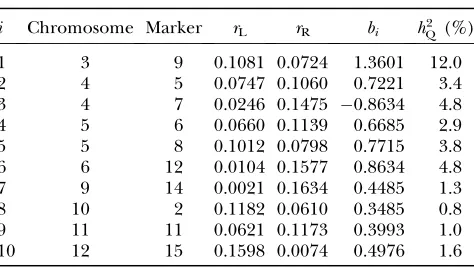
Data were simulated for a genome with 12 chromosomes of length 300 cM each for a total genome length ofG¼ 3600 cM, with markers located every 20 cM. The number and size of QTL effects were simulated with an average number of 10 additive QTL, total QTL heritability 35% (by which we mean the total variance of QTL is 35% of the within-family variance), and QTL sizes distributed with the default Gamma(2, 2) distribution. Backcross QTL mapping families with n ¼ 100, 300, and 1200 progeny were simulated and analyzed in separate runs with the same QTL and map configuration. Composite-interval mapping analyses (QTL Cartographer model 6) used the default values for window size (10 cM) and number of background markers (five). This means that for each test locus, five control markers are selected as covariates to control for possible QTL at other locations, and the control markers were selected from all geno-typed markersexceptthose within 10 cM of the test locus. The QTL effects simulated by QTL Cartographer were all positive in sign, corresponding to QTL in coupling, where there are more than one QTL on a chromosome. To make the data slightly more interesting, the QTL on chromosome 4 was replaced with two midsized QTL in repulsion. The total QTL heritability was inadvertently increased slightly but we continue to work with the nom-inal value of 35%. Individual QTL locations, effects, and heritabilities are shown in Table 1. QTL locations are given by chromosome, marker number for the left flank-ing marker, and recombination distancesrL andrR to
the left and right flanking markers, respectively. The
val-uesbiare the QTL effects. QTL Cartographer uses the
parameterization where
yi¼m1
X
j
xijbj1ei; ð21Þ
andxij¼1 (resp.xij¼0) if theith progeny hasjth QTL
genotypesQQ(resp.Qq). With this parameterization the
ith QTL variance isb2 i=4.
Priors for QTL effects: We give adjustments to the BIC for subjective priors for QTL effects with lower vari-ance. It is natural to specify the prior variance, s2
b, for
the QTL effects as a multiple of the trait genetic vari-ance,s2
G,
cbbiNð0;s2bÞ; where s2b ¼Ks2G; ð22Þ
where the constant cb is chosen so that the QTL
vari-ance for a single QTL is E((cbbi)2)¼s2b. For the QTL
Cartographer parameterization, the QTL variance is
b2
i=4 so we usecb¼12. Use ofcbin this way avoids
depen-dence on the parameterization. We refer to this prior as theindependence prior, since the effectsbiarea priori,
independent.
Recall that the QTL Cartographer parameterization uses effects QQ4bi, Qq40 for the ith QTL. For the
following argument we use the parameterization
yi¼m1
X
j
xijbj1ei; ð23Þ
where xij¼12(resp.xij¼ 12) if theith progeny hasjth
QTL genotypesQQ(resp.Qq). With this parameteriza-tion theith QTL variance is stillb2
i=4, and for unlinked
markers the columns ofXare uncorrelated and hence approximately orthogonal for large sample sizes. The Zellner prior is unchanged, because the Zellner prior is invariant to linear transformations of the parameter (i.e., if we replacebbyb*¼CbandXbyX*¼XC1, the transformed prior forb* is the Zellner prior withX re-placed byX*).
Since we are considering a prior distribution, rather than a particular sample, we take expected values over possible samples, obtaining a choice ofcwith expected values of QTL variances agreeing with those of the inde-pendence prior (22). The expected values will approx-imate estapprox-imates based on averages over rows of X for large sample sizes. For unlinked QTL, we choosecin the Zellner prior (18) so that the Zellner prior has the same expected QTL genetic variances for each individual QTL as the independence prior with the desired value ofKin (22). In the general case the Zellner prior will have the same total expected QTL variances,i.e., variance of the second term in (23), for each set of linked QTL as the independence prior with the chosen value ofK.
For unlinked QTL the QTL variances in the Zellner prior can be simply computed from the diagonal elements ofX9X. The QTL variances are the diagonal elements of
TABLE 1
QTL heritabilities and map positions
i Chromosome Marker rL rR bi hQ2 (%)
1 3 9 0.1081 0.0724 1.3601 12.0
2 4 5 0.0747 0.1060 0.7221 3.4
3 4 7 0.0246 0.1475 0.8634 4.8
4 5 6 0.0660 0.1139 0.6685 2.9
5 5 8 0.1012 0.0798 0.7715 3.8
6 6 12 0.0104 0.1577 0.8634 4.8
7 9 14 0.0021 0.1634 0.4485 1.3
8 10 2 0.1182 0.0610 0.3485 0.8
9 11 11 0.0621 0.1173 0.3993 1.0
c(X9X)1s2. For X corresponding to a set of unlinked QTL the columns ofX are orthogonal, and the diag-onals of (X9X)1are the inverses of the diagonals ofX9X. With the parameterization (23), the diagonals ofX9Xare
n/4. It follows that
s2b ¼varðcbbiÞ ¼ 1
4varðbiÞ ¼ 1 43
4c n s
2 ¼cs2=n: ð24Þ
For sets of mutually linked QTL the diagonals of (X9X)1will be smaller than the inverses of the diagonals ofX9X. For this case we give a more general derivation independent of the parameterization. The genetic var-iance due to QTL is the varvar-iance of the second term in (23),
VgðXÞ ¼var X
j
xijbj
!
¼XðcðX9XÞ1s2ÞX9
¼cXðX9XÞ1
X9s2; ð25Þ
which is ann3 nvariance–covariance matrix for sam-ples. The genetic variance is either approximately the average diagonal element from a large sample or the ex-pected value of any diagonal element.
First, consider the case of a single QTL. For a single QTL the matrixX has only 1 column, andi,jentry of
X(X9X)1X9is
VgðXÞij ¼cs2
xixj
P
kxk2
with EðVgðXÞijÞ ¼cs2=n
ifi ¼j; ð26Þ
i.e., the expected QTL variance is cs2/n, which agrees with (24). This does not depend on any of thexiso is the
same for all QTL. Therefore, withkindependent QTL loci, the total QTL genetic variance isktimes this value;
i.e.,
EðVgðXÞiiÞ ¼kcs2=n: ð27Þ In the general case we can choose the transformation
Ccorresponding to the Gram–Schmidt orthogonaliza-tion procedure, reducing the columns ofX to orthog-onality. It follows that (27) also applies in the general case. Q.E.D.
The prior variance for anykQTL from the indepen-dence prior isks2
b¼kKs2G. Equating this to the value for
the Zellner prior gives
kKs2G¼kcs2=n ð28Þ so that
c ¼ns
2
b s2 ¼
nKs2G s2 ¼nK
h2
1h2: ð29Þ
Equation 29 assumes that all of the genetic variance is accounted for by QTL. If there is prior information on the proportion of variance from nonadditive, epistatic,
and polygenic components this can be allowed for by choosing a smaller value ofKin (22).
The marginal probability of the data for a linear modelMis given by
fðyj MÞ}RSSn=2 1 11c p=2
; ð30Þ
wherec is as in Equation 18, RSS denotes the residual sum of squares after fitting the model,nis the number of sample points,pis the number of explanatory variables in the model, and the proportionality constant is inde-pendent of the model matrixX(cf.Senand Churchill
2001, Appendix C, where a there corresponds to 1/c
here). Taking logs and multiplying by2 gives the equi-valent value for the BIC,
BICnlogð1R2Þ1plogc; ð31Þ where we have used log(RSS) ¼ log(1 R2) 1 log(var(y)) ¼ log(1 R2) 1 const., c 1 1 c, and BIC¼ 2 logfðyj MÞup to an additive constant. The constant is chosen in (31) so that BIC¼0 for the null model with intercept alone (p¼0 andR2¼0). Posterior probabilities are unaffected by the choice of constant, because of the normalization of total probability to 1 when probabilities are calculated from (12).
To adjust the BIC for the prior for QTL effects cor-responding to c in (18) replacep logn byp log c, or, equivalently, add p log(c/n) to the BIC criterion. Ex-pressed in terms ofKandh2, this becomes
BICK ¼nlogð1R2Þ1plogn1plog K
h2
1h2
:
ð32Þ
Bromanand Speed(2002) use the adjusted criterion
BICd¼nlogð1R2Þ1dplogn: ð33Þ Using (32) is equivalent to setting
d¼11logðKðh
2=ð1h2ÞÞÞ
logn ð34Þ
in (33). For example, withK¼1
10,n¼1200, andh2¼0.35
we obtain
c ¼nK h 2
1h2 ¼0:0538n¼64:6; ð35Þ
andd¼0.59.
RESULTS
Worked example:Thummaet al.(2005) studied
associ-ations between SNPs and haplotypes in a candidate gene
between markers SNP18 and SNP120 in the same gene and MFA in Eucalyptus families (used as validation pop-ulations) were reported.
On the basis of the reported sample sizes, allele fre-quencies, and percentage of variance explained, Bayes factors for the candidates were calculated using the method of Spiegelhalter and Smith for one-way ANOVA models (Spiegelhalterand Smith1982; Ball2007).
Results are summarized in Table 2.
To illustrate the QTL colocation calculations suppose the candidate SNP21 (with Bayes factorBc¼98.4) is on
chromosome 3 with map position 170 cM, estimated with a normal posterior distribution with standard error 10 cM, and the QTL data available are the simulated QTL data withn¼300 as described above.
We assume prior probability pc ¼ 1/50,000, corre-sponding to a prior expectation of 10 SNPs in 500,000 covering the genome, to be closest to one of 10 func-tional loci affecting the trait. Without using QTL infor-mation the posterior probability was 1.963103½solve
pc/(1pc)¼Bc3pc/(1pc) forpc;cf.Ball2007,
Table 8.9].
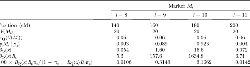
Chromosome 3 had one probable QTL located near marker 10, which had a posterior probability of 0.923. Table 3 shows calculations of quantities needed to eval-uate the posterior probabilities after allowing for QTL colocation.
Lettingx2V(Mi),
pQðxÞ ¼
gðMijyqÞ
jVðMiÞ
ð36Þ
pQðxÞ ¼
pQðVðMiÞÞ jVðMiÞ
ð37Þ
since the within-vicinity probabilities are assumed to be uniform, so
BQðxÞ ¼ pQðxÞ
pQðxÞ ¼ gðMijyqÞ
pQðVðMiÞÞ
:
ð38Þ
For example, for marker 10 at 180 cM we haveg(Mijyq)¼
0.923 (Table 5, ‘‘Total(%)’’ entry for marker 10 withn¼ 300), soBQ(x)¼0.923/0.0556¼16.6.
It remains to integrate over the probability density for map location, which is the normal density with mean 170 cM and standard deviation 10 cM;i.e.,
fðxjymÞ ¼
1
ffiffi
ð
p
2p3102Þexpððx170Þ
2=ð23102ÞÞ:
ð39Þ
Letting
Iða;bÞ ¼
ðb
a
fðxjymÞdx ð40Þ
the integral is given by
I¼ 1
100½0:0106Ið130;150Þ10:3143Ið150;170Þ13:1662Ið170;190Þ10:0142Ið190;210Þ ¼0:017;
ð41Þ
TABLE 2
Statistics for markers with ‘‘significant’’ associations with MFA from BALL(2007)
Population n Marker Frequency % var P B
E. nitensassociation population 290 SNP21 0.31 4.6 0.00023 98.4
E. nitensfamily 287 SNP18 0.5 0.45 0.02 1.5
E. globulusfamily 148 SNP120 0.5 0.69 0.04 1.1
Reprinted with permission from Ball(2007), Table 8.8, p. 152.
TABLE 3
Calculation of QTL colocation probabilities for candidate polymorphism SNP21, assumed to be located at 170 cM on chromosome 3, colocating with QTL from the simulated QTL mapping family withn¼300 progeny
MarkerMi
i¼8 i¼9 i¼10 i¼11
Position (cM) 140 160 180 200
jV(Mi)j 20 20 20 20
pQ(V(Mi)) 0.06 0.06 0.06 0.06
g(Mijyq) 0.003 0.089 0.923 0.004
BQ(x) 0.054 1.60 16.6 0.072
BQ(x)Bc 5.3 157.6 1634.8 6.71
1003BQ(x)Bcpc/(1pc1BQ(x)Bcpc) 0.0106 0.3143 3.1662 0.0142
where the coefficients ofI(a,b) terms in (41) are from the last row of Table 3.
Due to its colocation with the QTL on chromosome 3, the posterior probability for the candidate gene SNP21 has increased 8.5-fold to 0.017, which is still not high. Probabilities would increase further if the map location was known more precisely or the posterior probability for the QTL was higher. For example, if map position was known exactly to be 180 cM the posterior probability would rise to 0.032, representing a 16-fold increase in probability due to QTL colocation. Larger increases would require more accurate estimation of candidate map posi-tion and more accurate estimates of QTL posiposi-tion.
Note that in Thummaet al.(2005), the association was
considered ‘‘validated’’ by associations in theE. nitens
andE. globulus families (i.e., QTL data) with markers SNP18 and SNP128 (P¼0.02 and 0.04, respectively, in Table 2). This does not constitute validation at the level of resolution of an association study, but does represent evidence of colocation with a possible QTL. However, the Bayes factors of 1.5 and 1.1, respectively, are too small to make a significant difference.
Simulation results:Except where otherwise stated all Bayesian analyses for the simulated data use a prior prob-ability per marker based on an average number of 10 QTL per genome, and the standard BIC (equivalent to usingc¼nin the Zellner prior for QTL effects) is used to estimate posterior probabilities for models.
The posterior probability intensity for QTL presence,
pQ(x), is plotted against map position in Figure 1. Each
chromosome is plotted in a separate graph. Shown with the heading for each graph are the QTL herita-bilities (percentage of phenotypic variation) and mar-ginal probabilities for model sizes 0, 1, and 2 (p0,p1, and p2). Log-likelihood ratios for interval mapping and
composite-interval mapping are shown for comparison. The interval-mapping curves are high for a much wider region about the QTL thanpQ(x) while the
composite-interval-mapping curves are high for a slightly wider re-gion about the QTL thanpQ(x) at this sample size. The
curves are step functions because the posterior prob-ability for models with theith marker,Mi, selected is
shared equally among genomic locations inV(Mi)
(Equa-tion 14).
Figure1.—Posterior probability densitypQ(x) for QTL presence. Data were simulated for 12 chromosomes with genome length
G¼3600 cM,n¼1200 progeny, and 10 QTL with QTL heritabilities as shown. For each chromosome, marginal probabilities for models of size 0, 1, 2 QTL arep0,p1,p2, respectively. QTL locations are denoted with an asterisk. Likelihood ratios for interval
The probability,p0, for model size 0 is,0.001 for
chro-mosomes 3, 5, 6, 9, and 12, representing strong evidence for one or more QTL. These chromosomes had maxi-mum log-likelihood-ratio (LR) statistics.20 except for chromosome 4 with two QTL in repulsion, where the QTL at 87 cM is not detected by interval mapping or composite-interval mapping (LR ,10), and the com-posite-interval mapping peak is broader and centered to the left of the peak inpQ(x). The two QTL in repulsion
are clearly separated with a low value ofpQ(x) for the
intervening marker, and posterior probability for model size 2 was high (p2¼0.961), representing good evidence
for two QTL. For chromosome 3, with one QTL, and chro-mosome 5 with two QTL in coupling, there was strong evidence for one or more QTL (p0,0.001), but either
one- or two-QTL models were compatible with the data:
p1¼0.451,p2¼0.530 for chromosome 3, andp1¼0.562, p2¼0.412 for chromosome 5. For chromosome 3 the
two-QTL model probability is dominated by QTL at the two flanking markers (Table 5). This represents either one or two QTL to within the resolution of the marker map.
For chromosome 11, with one QTL withh2
Q ¼1%,
there was weak evidence for a QTL (p0¼0.12) or LR¼
10 and17 for IM and CIM.
For chromosome 12, with one QTL withh2
Q ¼1.6%,
there was strong evidence for a QTL (p0,0.001), but
one ‘‘fake’’ QTL at the left-hand end was ‘‘detected’’ by IM and CIM with likelihood ratios.10. The posterior probability for model size 2,p2 ¼0.744, was
approxi-mately three times greater thanp1¼0.229, representing
weak evidence for two QTL.
For chromosomes 1, 2, 7, and 8, where there was no QTL, the posterior probability for model size 0 was not low (0.654–0.966), as would be expected where there are no QTL.
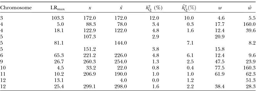
To show why we usepQ(x) rather than confidence
in-tervals, we illustrate the pitfalls in using a popular method for estimation of confidence intervals for QTL location. Table 4 shows estimated and actual heritabilities and confidence-interval widths calculated using the empir-ical formula of Darvasiand Soller(1997),
w¼ 3000
mNd2; ð42Þ
wherew is the confidence interval width for a QTL es-timated from a progeny of sizeN. The QTL is assumed to have an allele substitution effectd, andm¼1 for a backcross, andm¼2 for an F2. We have shown all
dis-tinguishable peaks down to LRmax¼4.5, not just those
over a demanding threshold. Confidence interval widths arew, based on the true QTL effect sizes, andwˆbased on QTL effect sizes estimated from the same data. Note there are some large differences betweenwandwˆdue to the QTL effects being under- or overestimated. Note also for chromosome 5, where there are two QTL but only one detected, we have wˆ¼8:2, compared tow¼ 20.9 andw¼15.8 for each of the two QTL and together spanning a 62-cM region. This will happen whenever two QTL in coupling are detected as a single QTL. For chromosome 4, one of the QTL had an LRmaxof only 5.0
and its heritability was underestimated by 10-fold. To-gether these confidence intervals span a region of 160 cM, compared with two regions of combined size 29 cM, when the true QTL effect sizes were used. This hap-pened because the effects of the two QTL were under-estimated, which happened because the two QTL were in repulsion. For chromosome 3, the estimated C.I. width was only5 cM, which is less than our intermarker spacings. This suggests we could do better in this case by using the Darvasi and Soller formula or using virtual markers to subdivide the region. However, bearing in
TABLE 4
Heritabilities and confidence-interval widths for putative QTL from interval mapping
Chromosome LRmax x ˆx h2Q(%) ˆh
2
Qð%Þ w wˆ
3 103.3 172.0 172.0 12.0 10.0 4.6 5.5
4 5.0 88.3 78.0 3.4 0.3 17.7 160.0
4 18.1 122.9 122.0 4.8 1.6 12.4 39.6
5 107.3 2.9 20.9
5 81.1 144.0 7.1 8.2
5 151.2 3.8 15.8
6 65.3 221.2 226.0 4.8 6.1 12.4 9.6
9 26.7 260.3 254.0 1.3 2.5 47.5 23.9
10 4.5 33.2 22.0 0.8 0.4 77.5 160.3
11 10.2 206.9 190.0 1.0 1.0 61.9 62.3
12 13.1 4.0 0.0 1.2 51.3
12 25.4 299.1 298.0 1.6 2.2 38.4 28.3
LRmax, the maximum log-likelihood for a peak;xandˆx, the true QTL position and its estimate;h2Q(%) and
ˆh2
Qð%Þ, the QTL heritability as a percentage of phenotypic variance and its estimate;wandwˆ, QTL confidence
interval widths based on the true and estimated QTL effects, calculated using the method of Darvasiand
Soller(1997) (Equation 42). Cells are left blank where a QTL did not exist corresponding to a peak or where
mind the results for chromosomes 4 and 5, caution is needed because we cannot rule out multiple QTL within the interval from 160 to 180 cM (the combined marker vicinities). If there were two QTL,e.g., at 167 and 173 cM with about half the variance each, their com-bined Darvasi and Soller confidence intervals would span a region of$20 cM. We conclude that we cannot rely on confidence intervals for QTL location, consid-ering QTL location separately, but need to consider the joint probability distributions for QTL existence, QTL effects, and QTL location, as in our approach.
Output from our method consists of a set of models with posterior probabilities and summary statistics, such as the marginal probability for each marker (total prob-ability of all models with the marker selected), and mar-ginal probabilities for model size (total probability of
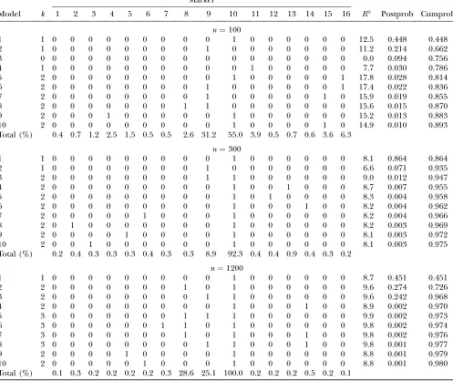
all models with the given size). These are shown for the top 10 markers for chromosomes 3 and 5 in Tables 5 and 6.
Top 10 models for chromosome 3:For chromosome 3, the top 10 models for each sample size are shown in Table 5. The first column is model number, in order of decreasing probability. The second column gives model size,k, while the next 16 columns show which markers are selected. The final 3 columns show theR2statistic, posterior probability per model, and cumulative sum of posterior probabilities for models. For example, forn¼ 300, model 1 with posterior probability 0.864 has marker 10 selected, model 2 with posterior probability 0.071 has marker 9 selected, and model 3 with posterior proba-bility 0.01. Model 3 (model sizek¼2) has higherR2than models 1 and 2 but lower posterior probability because
TABLE 5
Top 10 models for chromosome 3
Marker
Model k 1 2 3 4 5 6 7 8 9 10 11 12 13 14 15 16 R2 Postprob Cumprob
n¼100
1 1 0 0 0 0 0 0 0 0 0 1 0 0 0 0 0 0 12.5 0.448 0.448
2 1 0 0 0 0 0 0 0 0 1 0 0 0 0 0 0 0 11.2 0.214 0.662
3 0 0 0 0 0 0 0 0 0 0 0 0 0 0 0 0 0 0.0 0.094 0.756
4 1 0 0 0 0 0 0 0 0 0 0 1 0 0 0 0 0 7.7 0.030 0.786
5 2 0 0 0 0 0 0 0 0 0 1 0 0 0 0 0 1 17.8 0.028 0.814
6 2 0 0 0 0 0 0 0 0 1 0 0 0 0 0 0 1 17.4 0.022 0.836
7 2 0 0 0 0 0 0 0 0 1 0 0 0 0 0 1 0 15.9 0.019 0.855
8 2 0 0 0 0 0 0 0 1 1 0 0 0 0 0 0 0 15.6 0.015 0.870
9 2 0 0 0 1 0 0 0 0 0 1 0 0 0 0 0 0 15.2 0.013 0.883
10 2 0 0 0 0 0 0 0 0 0 1 0 0 0 0 1 0 14.9 0.010 0.893
Total (%) 0.4 0.7 1.2 2.5 1.5 0.5 0.5 2.6 31.2 55.0 3.9 0.5 0.7 0.6 3.6 6.3
n¼300
1 1 0 0 0 0 0 0 0 0 0 1 0 0 0 0 0 0 8.1 0.864 0.864
2 1 0 0 0 0 0 0 0 0 1 0 0 0 0 0 0 0 6.6 0.071 0.935
3 2 0 0 0 0 0 0 0 0 1 1 0 0 0 0 0 0 9.0 0.012 0.947
4 2 0 0 0 0 0 0 0 0 0 1 0 0 1 0 0 0 8.7 0.007 0.955
5 2 0 0 0 0 0 0 0 0 0 1 0 1 0 0 0 0 8.3 0.004 0.958
6 2 0 0 0 0 0 0 0 0 0 1 0 0 0 1 0 0 8.2 0.004 0.962
7 2 0 0 0 0 0 1 0 0 0 1 0 0 0 0 0 0 8.2 0.004 0.966
8 2 0 1 0 0 0 0 0 0 0 1 0 0 0 0 0 0 8.2 0.003 0.969
9 2 0 0 0 0 1 0 0 0 0 1 0 0 0 0 0 0 8.1 0.003 0.972
10 2 0 0 1 0 0 0 0 0 0 1 0 0 0 0 0 0 8.1 0.003 0.975
Total (%) 0.2 0.4 0.3 0.3 0.3 0.4 0.3 0.3 8.9 92.3 0.4 0.4 0.9 0.4 0.3 0.2
n¼1200
1 1 0 0 0 0 0 0 0 0 0 1 0 0 0 0 0 0 8.7 0.451 0.451
2 2 0 0 0 0 0 0 0 1 0 1 0 0 0 0 0 0 9.6 0.274 0.726
3 2 0 0 0 0 0 0 0 0 1 1 0 0 0 0 0 0 9.6 0.242 0.968
4 2 0 0 0 0 0 0 0 0 0 1 0 0 0 1 0 0 8.9 0.002 0.970
5 3 0 0 0 0 0 0 0 1 1 1 0 0 0 0 0 0 9.9 0.002 0.973
6 3 0 0 0 0 0 0 1 1 0 1 0 0 0 0 0 0 9.8 0.002 0.974
7 3 0 0 0 0 0 0 0 1 0 1 0 0 0 1 0 0 9.8 0.002 0.976
8 3 0 0 0 0 0 0 0 0 1 1 0 0 0 1 0 0 9.8 0.001 0.977
9 2 0 0 0 0 1 0 0 0 0 1 0 0 0 0 0 0 8.8 0.001 0.979
10 2 0 0 0 0 0 1 0 0 0 1 0 0 0 0 0 0 8.8 0.001 0.980
Total (%) 0.1 0.3 0.2 0.2 0.2 0.2 0.3 28.6 25.1 100.0 0.2 0.2 0.2 0.5 0.2 0.1
of the penalty term in the BIC and because the prior probability per marker is,0.5.
For n ¼1200, the top three models accounted for 97% of the probability, and marker 10 (at 180 cM) was selected in each of the top 10 models. In fact, marker 10 was selected in every model with nonnegligible proba-bility, with a marginal probability of very close to 100%. Markers 8 and 9 had marginal probabilities of 28.6 and 25.1%, respectively. Forn¼1200, the null model (not shown) had posterior probability,0.001, representing strong evidence for a QTL.
At smaller sample sizes there was, naturally, more var-iability. Forn¼300, the top three models accounted for 95% of the posterior probability. Marker 9 and/or 10 was selected in the top three models. Forn¼100, model
3, with model sizek¼0 had posterior probability (p0¼
0.09), representing weak to moderate evidence for a QTL, although markers 9 and 10 had the highest mar-ginal probabilities (31.2 and 55.0%, respectively), with 4% probability for marker 11.
For n ¼300, the highest-probability single model (model 1) with marker 10 selected had a posterior prob-ability of 0.864. The same model had the highest pos-terior probability forn ¼100 and 1200 but with lower posterior probability of 0.45. This has also resulted in less posterior variance of QTL location forn¼300, as is evident from the marginal probabilities for markers (Total % rows in Table 5). At first sight this seems coun-terintuitive, since as sample size increases the QTL location should be more accurately estimated, and the true model
TABLE 6
Top 10 models for chromosome 5
Marker
Model k 1 2 3 4 5 6 7 8 9 10 11 12 13 14 15 16 R2 Postprob Cumprob
n¼100
1 0 0 0 0 0 0 0 0 0 0 0 0 0 0 0 0 0 0.0 0.488 0.488
2 1 0 0 0 0 0 0 1 0 0 0 0 0 0 0 0 0 8.2 0.202 0.690
3 1 0 0 0 0 0 0 0 0 0 1 0 0 0 0 0 0 6.3 0.073 0.764
4 1 0 0 0 0 0 0 0 0 1 0 0 0 0 0 0 0 5.3 0.043 0.807
5 1 0 0 0 0 0 0 0 0 0 0 1 0 0 0 0 0 5.2 0.042 0.849
6 1 0 0 0 0 0 0 0 1 0 0 0 0 0 0 0 0 4.7 0.033 0.882
7 1 0 0 0 0 0 1 0 0 0 0 0 0 0 0 0 0 4.2 0.025 0.906
8 1 0 0 0 0 0 0 0 0 0 0 0 0 0 1 0 0 3.2 0.015 0.921
9 2 0 0 0 0 0 0 1 0 0 0 1 0 0 0 0 0 11.8 0.009 0.930
10 2 0 0 0 0 0 0 1 0 0 1 0 0 0 0 0 0 11.5 0.008 0.937
Total (%) 0.3 0.6 0.4 0.5 0.6 3.2 24.0 3.6 4.9 8.9 5.7 0.8 0.5 2.0 0.4 0.2
n¼300
1 1 0 0 0 0 0 0 0 0 1 0 0 0 0 0 0 0 9.1 0.626 0.626
2 2 0 0 0 0 0 0 1 0 1 0 0 0 0 0 0 0 11.4 0.102 0.728
3 2 0 0 0 0 0 1 0 0 1 0 0 0 0 0 0 0 11.0 0.054 0.782
4 2 0 0 0 0 0 0 1 0 0 1 0 0 0 0 0 0 10.9 0.043 0.826
5 1 0 0 0 0 0 0 0 0 0 1 0 0 0 0 0 0 7.3 0.037 0.862
6 1 0 0 0 0 0 0 1 0 0 0 0 0 0 0 0 0 7.2 0.028 0.891
7 2 0 0 0 0 0 0 0 0 1 1 0 0 0 0 0 0 10.2 0.014 0.905
8 2 0 0 0 0 1 0 0 0 1 0 0 0 0 0 0 0 10.1 0.012 0.917
9 2 0 0 1 0 0 0 0 0 1 0 0 0 0 0 0 0 10.1 0.011 0.928
10 2 0 0 0 0 0 1 0 0 0 1 0 0 0 0 0 0 9.8 0.008 0.936
Total (%) 0.1 0.5 1.4 0.8 1.3 6.6 18.5 2.1 86.3 11.7 0.5 0.4 0.2 0.5 0.3 0.1
n¼1200
1 1 0 0 0 0 0 0 0 1 0 0 0 0 0 0 0 0 7.6 0.562 0.562
2 2 0 0 0 0 0 1 0 1 0 0 0 0 0 0 0 0 8.4 0.159 0.720
3 2 0 0 0 0 0 0 1 1 0 0 0 0 0 0 0 0 8.4 0.145 0.865
4 2 0 0 0 0 0 0 1 0 1 0 0 0 0 0 0 0 8.3 0.070 0.935
5 2 0 0 0 0 0 0 0 1 1 0 0 0 0 0 0 0 8.1 0.021 0.957
6 3 0 0 0 0 0 1 0 1 1 0 0 0 0 0 0 0 8.9 0.006 0.963
7 3 0 0 0 0 0 0 1 1 1 0 0 0 0 0 0 0 8.9 0.006 0.970
8 2 0 0 0 0 0 0 0 1 0 0 0 0 0 1 0 0 7.8 0.004 0.973
9 2 0 0 0 0 0 0 0 1 0 0 1 0 0 0 0 0 7.7 0.002 0.975
10 2 0 0 0 0 0 0 0 1 0 1 0 0 0 0 0 0 7.7 0.002 0.977
Total (%) 0.1 0.2 0.2 0.2 0.2 17.3 22.9 92.7 10.7 0.3 0.4 0.2 0.2 0.7 0.2 0.1
should be selected with probability asymptotically ap-proaching 1. However, here we are not in the asymptotic situation—sample sizes are not large enough to select a single best model, nor is model 1 the true model, since the true QTL location is intermediate between markers 9 and 10. The probabilities 0.864 and 0.45 are inter-mediate probabilities, and the differences between them can easily occur by chance,e.g., as a result of fewer re-combinations between the QTL and marker 10 forn¼ 300 than for the other two sample sizes.
Top 10 models for chromosome 5:For chromosome 5, the top 10 models for each sample size are shown in Table 6. Forn¼1200, the top 3 models accounted for 86% of the probability. As was the case for chromosome 3, the probability for model size 0 was,0.001, corre-sponding to strong evidence for one or more QTL on this chromosome, and models of size 1 and 2 shared the probability approximately equally. Unlike chromosome 3, the probability for models of size 2 was not concen-trated at adjacent markers.
Forn¼1200, markers 6–9 had marginal probabilities
.1%, corresponding to a region of 80 cM for the double QTL. For n ¼ 300 and 100 this region expanded to 120 cM.
Posterior probabilities for candidate gene polymor-phisms:Candidate gene polymorphisms were not sim-ulated; rather, we consider hypothetical candidate gene polymorphisms with various values ofBc, at various
ge-nomic locations. To illustrate the method we plot the posterior probabilities for the candidates after incorpo-rating QTL colocation information from the simulated QTL data, as a function of genomic location. Posterior probabilities for the candidate genes are calculated us-ing Equation 8. A standard error of 3 cM (as would be obtained with a mapping population of size 100 and marker spacing of 20 cM) for estimated map location of candidate genes was assumed.
Figure 2 is a plot of posterior probabilities for can-didate gene polymorphismsvs.estimated map position on chromosomes 2, 4, 5, and 11. There are separate curves corresponding to candidate polymorphisms with Bayes factorsBc¼20,Bc¼100, andBc¼400. The
pos-terior probability curves are ‘‘wavy,’’ because the inte-grand in (8) is the piecewise constant functionBQ(x)Bcpc/
(1pc1BQ(x)Bcpc) multiplied by the densityf(xjym)
of map location, which has the effect of smoothing the piecewise constant function. If the map location was known exactly the curves would look similar to the step functions in Figure 1.
Figure 3 similarly shows posterior probabilities for can-didate polymorphisms on chromosome 3 for various sample sizes.
Accuracy of the BIC: The Bayes factors correspond-ing to model probabilities estimated uscorrespond-ing the BIC are compared with the closed-form expressions for Bayes factors with the Zellner prior½Zellner 1986;c ¼n in
(18)in Figure 4 forn¼100, 300, and 1200. Differences,
indicated by deviations from the diagonals, are almost imperceptible, indicating good agreement.
Subjective priors for QTL effects: Figure 4 shows that the estimates of Bayes factors, and hence posterior probabilities based on the BIC, are very good approx-imations to the values withc¼nin Equation 18. How-ever,c ¼n in (18) corresponds to a prior variance of s2
b ¼s
2for QTL that can be greater than the genetic
variance. This is conservative, since QTL variances are generally only a fraction of the genetic variance, and the heritability is often approximately known.
Posterior probabilities for QTL presence for two priors are shown for chromosome 11 in Figure 5. Probabilities are calculated with the default prior withK¼1.86 (d¼1) and the subjective prior withK¼ 1
10(d¼0.59),
corre-sponding to an average QTL variance ofs2 G/10.
The probabilities for QTL presence at long distances from QTL loci have increased approximately twofold, but are still less than the posterior odds from the candi-date gene data alone.
DISCUSSION
We have shown how to calculate posterior probabil-ities for candidate gene polymorphisms by combining sequence-specific evidence for candidate genes with QTL colocation information. Our method takes into account uncertainty in number and locations of QTL on each chromosome and uncertainty in estimated map posi-tion. For candidate genes that map to QTL regions, this can result in substantially larger posterior probabilities. Where a number of candidate genes are available, among candidates with given Bayes factor Bc those that map
near a QTL are most promising for functional testing. QTL colocation is often specified as a candidate gene falling within a 95% confidence interval. Confidence intervals are formed by selecting a peak in the interval-mapping likelihood, assumed to represent a QTL. If QTL effects are known, or assumed (as in an experimen-tal design situation) or estimated from independent data, unbiased confidence intervals can be obtained using the simple formula of Darvasiand Soller(1997).
How-ever, QTL effects are seldom estimated from independent data, and estimates for significant effects are subject to selection bias. For example, only 2 of 20 QTL-mapping experiments in forest trees, reviewed by Sewell and
Neale (2000), used an independent verification
pop-ulation. Estimates of QTL effects free of selection bias can be obtained in the Bayesian model-selection ap-proach (Ball 2001), but in this approach we do not
consider the number and locations of QTL, and size of their effects, as in our approach.
Bayes factors and posterior probabilities for QTL presence in a small interval were calculated on the basis of the output of QTL analysis using Bayesian model selection on the set of linear regression models with sets of selected markers as variables. As in Ball(2001),
pos-terior probabilities for models were obtained using the
BIC. Comparison with closed-form expressions for Bayes factors for comparing pairs of models with Zellner priors showed that the BIC approximation was very good for the sample sizes considered (n $100 QTL-mapping progeny).
Why not just use Bayes factors?In principle, the BIC is not needed—if using Zellner priors we could use the closed-form expressions for marginal probabilities of
Figure2.—Posterior probabilities for candidate gene polymorphisms by estimated map position forn¼1200 QTL progeny.
Values are shown for (a) chromosome 2, (b) chromosome 4, (c) chromosome 5, and (d) chromosome 11. Each line shows pos-terior probabilities as a function of estimated map position for a given Bayes factorBc, forBc¼1, 20, 100, 400, representing
the data, and from these compute Bayes factors for pairs of models, and hence compute posterior probabilities directly without using the BIC. As we have seen, the ad-justed BIC is essentially equivalent to probabilities from the Zellner prior for reasonably large QTL-mapping
sample sizes. The BIC is used mainly for convenience and compatibility with existing software—it is easily com-puted from standard linear model software output,e.g., leaps and regsubsets in R and Splus, and is used in the bicreg S function (Raftery1995; Rafteryet al.1997)
Figure3.—Posterior probabilities for candidate gene polymorphisms by estimated map position for chromosome 3. Values are
shown for (a)n¼100, (b)n¼300, and (c)n¼1200 QTL progeny. Each line shows posterior probabilities as a function of estimated map position for a given Bayes factorBc, forBc¼1, 20, 100, 400, representing sequence-specific evidence for a candidate
for Bayesian model selection in linear models using the BIC. Moreover, the Zellner prior is not a natural subjec-tive prior, with prior covariance between linked markers similar to the likelihood and with prior variance pro-portional tos2—we do not necessarily recommend its use in any given situation.
The Bayes factor does not depend on the prior prob-ability per marker but does depend on the prior dis-tribution of the parameter(s) being tested. Bromanand
Speed(2002) introduced the extra penalty factor din
the BIC and recommendedd¼2, 3, possibly allowing for asymptotics and, in the frequentist paradigm, multi-ple comparisons. We have seen here that when we allow for prior probabilities per marker,d¼1 corresponds to a good generally useable, but conservative, default prior for QTL effects, with information approximately equiv-alent to one sample point. Where there is lower prior variance for QTL effects, higher Bayes factors and
pos-terior probabilities will be obtained, so it is worth using this prior information if available.
We have shown how to modify the BIC to enable specification of a subjective prior for QTL effects with prior variance for QTL effects specified as a multiple of the within-family genetic variance, corresponding tod,
1,e.g.,d¼0.59, corresponding to average QTL variances of one-tenth of the genetic variance for the simulated data set. Even lower values could be used if, for example, preliminary QTL studies have been carried out, so that remaining undetected QTL are likely to be small. How-ever, comparison betweend¼1 andd¼0.59 did not show a major difference—with the main apparent difference being larger posterior probabilities for candidates lo-cated farther from the QTL position: in this case the sen-sitivity to prior variance was not high. This is apparently paradoxical, because one would ‘‘like’’ posterior prob-abilities to be higher at the QTL and lower far from the
Figure 4.—Accuracy of the BIC
approxima-tion. The logarithm of Bayes factors calculated from the BIC is plotted against the logarithm of Bayes factors calculated using the closed-form expression from Smithand Kohn (1996) with
the Zellner prior½c¼nin (18)forn¼100,n¼
300, andn¼1200 QTL progeny. Differences be-tween the two Bayes factors are shown as deviations from the diagonal lines.
Figure 5.—Posterior probabilities for
candi-date gene polymorphisms by estimated map posi-tion for chromosome 11. Values are shown for (a) d¼1, corresponding to a prior withc¼nin (18) or a prior with QTL variance ofs2
b ¼s
2, with
in-formation equivalent to half a sample point, and (b)d¼0.59, corresponding toc¼ 1
10nh
2=ð1h2Þ
in (18) or a prior with QTL variance of 1 10s
QTL. However, using a more informative prior for the parameter being tested raises the Bayes factors for all loci, at least where the evidence from the QTL mapping is in favor of a QTL (B.1). Nevertheless, the subjective prior is still recommended, as giving a more ‘‘correct’’ posterior where prior information is available.
In the worked example, an 8.5-fold increase in pos-terior odds for the candidate was obtained, due to QTL colocation. The posterior probability for a QTL in the vicinity of marker 10 was 0.923, which is already fairly high; increasing it to,e.g., 0.999 would yield only modest increases in posterior odds for the candidate. Larger in-creases are possible given more accurate candidate map locations and QTL locations. This would require both larger QTL-mapping sample sizes and more dense marker spacings. For example, if the marker spacing was 0.2 cM, the candidate was accurately mapped to marker 10, and the posterior probability for a QTL in the vicinity of marker 10 was 0.9, the posterior probability for the candidate would rise to 0.48, representing a 243-fold increase in probability due to QTL colocation.
In spite of a Bayes factor of 98.4 and a further 8.5-fold increase in odds due to QTL colocation, the posterior probabilities for the candidate were still not high. This is because we have used low prior probabilities. Thumma
et al.(2005) tested 25 SNP markers within the candidate gene and gaveP-values adjusted for the number of tests. For this to be relevant amounts to a tacitprior assumption
that at least one real effect is present within the gene with high probability. (Here, as is common in other ex-amples, the frequentist analysis also uses prior infor-mation, albeit poorly quantified and nontransparently.) However, we see no reason why the gene should directly affect the trait in question (MFA); hence we have used low prior odds appropriate for a random candidate. The number of loci tested, or that might be tested, affects the
P-values, but does not govern the posterior probabilities— hence our assertion: QTL and association mapping are model-selection problems, not multiple-testing problems. The posterior probabilities for QTL presence were compared to interval mapping and composite-interval mapping. The composite-interval mapping curves were qualitatively similar to the posterior probabilities, in that, where evidence for a QTL was strong, the composite-interval mapping curves were high in a region similar to or slightly wider than the region with high posterior probability for a QTL, while interval-mapping curves were high for a substantially wider region. This is not surpris-ing since our approach tests for a QTL within a small regionvs.the null hypothesis of no QTL in that region, but for possible QTL anywhere else, while interval map-ping tests for a QTL at a locationvs.no QTL anywhere. Composite-interval mapping attempts to allow for possi-ble QTL elsewhere by conditioning on a set of auxiliary marker genotypes. If there is an auxiliary marker be-tween the location being tested and another QTL, then the effect of the other QTL will be absorbed by the
auxiliary marker. (Conditional on the auxiliary marker genotype, the genotypes for the marker being tested are independent of the QTL genotype.) Where there are two or more reasonably close QTL on a chromosome, composite-interval mapping may not choose a suitable auxiliary marker. For example, the two QTL on chro-mosome 4 in our simulated data were not resolved by composite-interval mapping. The effectiveness, or oth-erwise, of composite-interval mapping hinges on the choice of auxiliary markers to condition on—auxiliary markers can absorb the effect of the QTL being tested as well as other QTL, and estimating coefficients for the auxiliary markers can add error, as well as reduce resi-dual variation. The optimal choice of number and loca-tion of auxiliary markers depends on unknown localoca-tions and magnitudes of QTL effects; hence mixed results for CIM are reported by Bromanand Speed(2002). Bayesian
model selection does, optimally, in a coherent mathe-matical framework, based on interpretable prior distri-butions, what composite-interval mapping attempts to do in anad hocway with arbitrary choices.
In our simulated data, chromosome 4 had two QTL in repulsion. For n ¼1200 QTL progeny, these were strongly detected and well separated by the Bayesian model-selection method but not by composite-interval mapping or interval mapping. It is important to detect QTL pairs in repulsion—QTL in repulsion represent an important source of latent variation, particularly for traits of undomesticated species that have been subject to stabilizing selection, which could be exploited by fu-ture selection or QTL mapping. We note that the QTL effects simulated by QTL Cartographer (Bastenet al.
1994, 2004) were all positive in sign, whereas in many cases there would be a number of QTL pairs in repul-sion. This means that many QTL Cartographer-based simulations may be optimistic.
As in QTL Cartographer, the within-family variation was assumed to be fully accounted for by QTL. In prac-tice, nonadditive, epistatic, and polygenic components may reduce the proportion of genetic variance due to QTL. Prior information on these terms can be allowed for if known; otherwise the prior variance for QTL ef-fects will be slightly larger. This is conservative, since Bayes factors reduce when there is weaker prior information for the size of effects being tested.
In our method, probabilitiespQ(x) are piecewise
con-stant in the vicinity of the nearest marker. This is not a major problem; however, if desired, the probabilities (14, 15) can be smoothed by applying a kernel smoother and renormalizing, so that the probability integral for each chromosome or linkage group is unchanged. Or, missing marker data can be estimated by multiple impu-tation (Ball2001). This was intended for markers where
marker genotypes were missing for some individuals, but can also be used for ‘‘virtual markers’’ with all data miss-ing (cf.Senand Churchill2001). One or more virtual
to obtain intermediate probabilities and hence smooth the graph of posterior probabilities. This is potentially useful if most of the posterior probability for a QTL is concentrated around a single marker. There is, however, a limit to the benefit of adding virtual markers—a single QTL located between two markers is well represented by one QTL at each of two adjacent flanking markers with posterior probabilities for each marker reflecting the re-lative proximity of the QTL to each of the flanking mark-ers. To distinguish between these two possible genetic architectures requires moreactualmarkers.
Senand Churchill(2001) use closed-form expressions
for marginal probabilities for linear models to estimate a joint posterior probability density for QTL locations for a set of QTL. In their Figure 2 and Appendix D they note the log posterior densities for QTL location and the LOD scores calculated using the EM algorithm were very similar. This is surprising, since we have seen that the interval-mapping likelihood ratios give excessively wide intervals around QTL. In fact, it is an error to estimate QTL location from probabilities of models with a fixed number of QTL. Their log posterior density and LOD scores are similar because,when restricting to a fixed number of QTL, the BIC is the same as the log likelihood or LOD score up to a constant, and the sample sizes are such that the BIC gives good approximations to marginal probabilities for models. Their posterior density for QTL location is not the same aspQ(x), since they assume a
fixed number of QTL per chromosome. We have seen that the number of QTL on a linkage group may not be unequivocally determined (e.g., Figure 1, chromosomes 5 and 12); hence there is the need to incorporate model uncertainty in both the number and the locations of QTL. When considering models of different size we often see that models of size 2 (e.g., Table 2,n¼1200) dominate models of size 1 except for the model with only the marker closest to the QTL selected, resulting in a sharper drop-off inpQ(x) than the LOD score. In other words, when
testing for a QTL at a given location one has to allow for possible QTL at other locations, which entails models of size 2 or more.
There are various possible experimental strategies for gene discovery combining, for example, information from association studies and QTL-mapping studies. Depend-ing on sample size and size of QTL effects, most QTL-mapping studies have a resolution of tens of centimorgans for QTL location (Tables 5 and 6 anddiscussion).
Pre-liminary results for genome scans (Ball 2007) suggest
that not only is QTL-mapping information useful, but prior to association studies it is more efficient to do an even larger QTL-mapping study than most QTL-mapping studies (e.g., with n ¼ 3000 QTL-mapping progeny for small QTL effects). For candidate genes, graphs of posterior probability for different sample sizes (cf. Fig-ure 4) could be used to find the optimal design; however, in the absence of a theoretical power calculation, many replicate simulations are needed.
The author thanks Phillip Wilcox and the Scion Cell Wall Bio-technology Center for supporting this work and Rowland Burdon and the referees for useful comments that improved the manuscript. This work was funded by the New Zealand Foundation for Research, Sci-ence, and Technology through a contract with the New Zealand Forest Research Institute.
LITERATURE CITED
Ball, R. D., 2001 Bayesian methods for quantitative trait loci
map-ping based on model selection: approximate analysis using the Bayesian information criterion. Genetics159:1351–1364. Ball, R. D., 2007 Statistical analysis and experimental design, pp.
133–196 inAssociation Mapping in Plants, edited by N. C. Oraguzie,
E. H. A. Rikkerink, H. N. DeSilvaand S. E. Gardiner. Springer,
New York.
Basten, C. J., B. S. Weirand Z.-B. Zeng, 1994 Zmap a QTL
cartog-rapher, pp. 65–66 inProceedings of the 5th World Congress on Genetics Applied to Livestock Production: Computing Strategies and Software, Vol. 22, edited by C. Smith, J. S. Gavora, B. Benkel, J. Chesnais,
W. Fairfull, J. P. Gibson, B. W. Kennedyand E. B. Burnside.
5th World Congress on Genetics Applied to Livestock Produc-tion, Guelph, Ontario, Canada.
Basten, C. J., B. S. Weirand Z.-B. Zeng, 2004 QTL Cartographer, Ver-sion 1.17.North Carolina State University, Raleigh, NC. Bennewitz, J., N. Reinschand E. Kalm, 2002 Improved confidence
intervals in quantitative trait loci mapping by permutation boot-strapping. Genetics160:1673–1686.
Bogdan, M., J. K. Ghoshand R. W. Doerge, 2004 Modifying the
Schwarz Bayesian information criterion to locate multiple inter-acting quantitative trait loci. Genetics167:989–999.
Broman, K., 1997 Identifying quantitative trait loci in experimental
crosses. Ph.D. Thesis, University of California, Berkeley, CA. Broman, K., and T. Speed, 2002 A model selection approach for the
identification of quantitative trait loci in experimental crosses. J. R. Stat. Soc. B64:641–656, 731–775.
Darvasi, A., and M. Soller, 1997 A simple method to calculate
resolving power and confidence interval of QTL map location. Behav. Genet.27:125–132.
Jansen, R. C., and P. Stam, 1994 High resolution of quantitative traits
into multiple loci via interval mapping. Genetics136:1447–1455. Kass, R. E., and L. Wasserman, 1995 A reference Bayesian test for
nested hypotheses and its relationship to the Schwarz criterion. J. Am. Stat. Assoc.90:928–934.
Lander, E., and D. Botstein, 1989 Mapping Mendelian factors
un-derlying quantitative traits using RFLP linkage maps. Genetics
121:185–199.
Manichaikul, A., J. Dupuis, S. Senand K. W. Broman, 2006 Poor
performance of bootstrap confidence intervals for the location of a quantitative trait locus. Genetics174:481–489.
Raftery, A., 1995 Bayesian model selection in social research, pp.
111–196 in Sociological Methodology, edited by P. V. Marsden.
Blackwell, Cambridge, MA.
Raftery, A., D. Madiganand J. A. Hoeting, 1997 Bayesian model
aver-aging for linear regression models. J. Am. Stat. Assoc.92:179–191. Sen, S., and G. Churchill, 2001 A statistical framework for
quan-titative trait mapping. Genetics159:371–387.
Sewell, M. M., and D. Neale, 2000 Mapping quantitative traits in
forest trees, pp. 407–424 inMolecular Biology of Wood Plants, edited by S. M. Jainand S. C. Minocha. Kluwer Academic Publishers,
Dordrecht, The Netherlands.
Sillanpa¨ a¨, M. J., and J. Corander, 2002 Model choice in gene
map-ping: what and why. Trends Genet.18:301–307.
Spiegelhalter, D., and A. Smith, 1982 Bayes factors for linear and
log-linear models with vague prior information. J. R. Stat. Soc. Ser. B44(3): 377–387.
Smith, M., and R. Kohn, 1996 Nonparametric regression using
Bayesian variable selection. J. Econ.75:317–343.
Thumma, B. R., M. F. Nolan, R. Evansand G. G. Moran, 2005
Polymor-phisms inCinnamoyl CoA Reductase(CCR) are associated with varia-tion in microfibril angle in Eucalyptus spp. Genetics171:1257–1265. Visscher, P. M., R. Thompsonand C. S. Haley, 1996 Confidence
Yandell, B. S., C. Jin, J. M. Satagopan and P. J. Gaffney,
2002 Discussion of: model selection approach for the identifi-cation of quantitative trait loci in experimental crosses, by Bro-man and Speed. J. R. Stat. Soc. Ser. B64:731–775.
Yi, N., V. Georgeand D. B. Allison, 2003 Stochastic search variable
selection for identifying multiple quantitative trait loci. Genetics
164:1129–1138.
Zellner, A., 1986 On assessing prior distributions and Bayesian
regression analysis with g-prior distributions, pp. 233–243 in
Bayesian Inference and Decision Techniques, edited by P. K. Goel
and A. Zellner. Elsevier Science, New York.
Zeng, Z.-B., 1993 Theoretical basis for separation of multiple linked
gene effects in mapping quantitative trait loci. Proc. Natl. Acad. Sci. USA90:10972–10976.
Zeng, Z.-B., 1994 Precision mapping of quantitative trait loci.
Genetics136:1457–1468.