Combined Economic Environment Unit
Commitment by Using Modified Water
Evaporation Optimization Algorithm
R. Anandhakumar
Assistant Professor, Department of Electrical & Electronics Engineering, Annamalai University, Annamalainagar,
Tamilnadu, India
ABSTRACT: Unit commitment which is considered as a large scale, nonlinear, mixed-integer optimization problem plays a very important role in optimal operation of power systems. Solving the UC problem is a complex decision-making process since multiple constraints must be satisfied and a good UC solution method can substantially contribute to annual savings of production cost. In this paper combined economic environment unit commitment by using modified water evaporation optimization algorithm has been proposed. In order to show the feasibility of the proposed algorithm it has been tested with 10 unit system and the results are compared with existing method.
KEYWORDS: Unit commitment, water evaporation optimization, Emission, Generation dispatch
I. INTRODUCTION
The objective of the UC problem is to minimize the total cost of thermal generating units while maintaining sufficient spinning reserve and satisfying the operational constraints of generating units over a given schedule time horizon [1]. Due to the increasing environmental protection the emission is also added to UC problems.
Over the years, extensive research has been conducted on developing efficient UC algorithm that can be mainly grouped as numerical based techniques and Heuristic search based techniques [2-27]. In this paper, combined economic environment unit commitment has been proposed using modified water evaporation optimization algorithm [26] are implemented to handling ramp rates with the aims of achieving the desired solution accuracy and to reduce the cost and emission computational effort in 24 hr time horizon.
II. PROBLEM FORMUATION
Multi-objective UC Model
T
t N
i
t i i t
i t i t i
i
P
SC
SD
h
E
P
FC
F
Min
1 1
*
(2.1)SDit is the Shutdown cost of the ith generator at t hour. F is the combined Fuel cost and Emission with penalty
Constraints
1. Power balance constraint
Power balance constraint states that, the generated power should be sufficient enough to meet the power demand
and is given by,
N
i
t i t
i
P
t
T
U
1,...,
2
,
1
(2.2)
2. Generated power limits constraint
The generated power of online generating units should lie between its upper and lower limits as given by,
t i i t i t i
i
U
P
P
U
P
,min
,max(2.3) Where Pi,min and Pi,max are the minimum and maximum thermal output power at ith unit.
3. Spinning reserve requirement constraint
Spinning reserve is essential to maintain system reliability; sufficient spinning reserve must be available at every
time period. Usually, the spinning reserve is given as some percentage of the total power demand.
N
i
t t i
t
i
P
LD
SR
U
1
max ,
(2.4)
Where SRt spinning reserve at hour t, LDt load demand during hour t.
4. Minimum up and down time constraint
This constraint helps to determine shortest time periods during which a unit must be on or down.
i off
t i
i on
t i
MD
HR
MU
HR
, ,
(2.5)
Where HRit,on and HRit,off are number of hours at unit i is continuously online and offline unit until tth hour. MUi is
the minimum up time hours and MDi is the minimum down time hours.
5. Ramp rate limit constraint
Because of the physical restrictions on thermal generating units, the rate of generation changes must be limited within certain ranges. The ramp rate limits confine the output movement of a generating unit between adjacent hours.
i t
i t i
i t
i t i
RD
P
P
RU
P
P
1 1
III. WATER EVAPORATION OPTIMIZATION ALGORITHM
The evaporation of water is very important in biological and environmental science. The water evaporation from bulk surface such as a lake or a river is different from evaporation of water restricted on the surface of solid materials. In this WEO algorithm water molecules are considered as algorithm individuals. Solid surface or substrate with variable wettability is reflected as the search space. Decreasing the surface wettability (substrate changed from hydrophility to hydrophobicity) reforms the water aggregation from a monolayer to a sessile droplet.
Such a behavior is consistent with how the layout of individuals changes to each other as the algorithm progresses. And the decreasing wettability of surface can represent the decrease of objective function for a minimizing optimization problem. Evaporation flux rate of the water molecules is considered as the most appropriate measure for updating individuals which its pattern of change is in good agreement with the local and global search ability of the algorithm and make this algorithm have well converged behavior and simple algorithmic structure. The details of the water evaporation optimization algorithm are well presented in (Kaveh and Bakhshpoori, 2016).
In the WEO algorithm, each cycle of the search consists of following three steps (i) Monolayer Evaporation Phase, this phase is considered as the global search ability of the algorithm (ii) Droplet Evaporation Phase, this phase can be considered as the local search ability of the algorithm and (iii) Updating Water Molecules, the updating mechanism of individuals.
(i) Monolayer Evaporation Phase
In the monolayer evaporation phase the objective function of the each individuals Fitit is scaled to the interval [-3.5,
-0.5] and represented by the corresponding Esub(i)t inserted to each individual (substrate energy vector), via the
following scaling function.
minmin max
E
Fit
Min
Fit
MaX
Fit
Min
Fit
E
E
i
E
t i t sub
(3.1)Where Emax and Emin are the maximum and minimum values of Esub respectively. After generating the substrate
energy vector, the Monolayer Evaporation Matrix (MEP) is constructed by the following equation.
t sub ij t sub ij t iji
E
rand
if
i
E
rand
if
MEP
exp
0
exp
1
(3.2)where MEPtij isthe updating probability for the jth variable of the ith individual or water molecule in the tth iteration
of the algorithm. In this way an individual with better objective function is more likely to remain unchanged in the search space.
(ii) Droplet Evaporation Phase
In the droplet evaporation phase, the evaporation flux is calculated by the following equation.
cos
1
cos
3
cos
3
2
3
J
oP
oJ
(3.3)
where Jo and Po are constant values. The evaporation flux value is depends upon the contact angle ϴ, whenever this
angle is greater and as a result will have less evaporation. The contact angle vector is represented the following scaling function.
minmin
max
Where the min and max are the minimum and maximum functions. The ϴmin & ϴmax values are chosen between
-50o <ϴ < -20o is quite suitable for WEO. After generating contact angle vector ϴ(i)t the Droplet Probability Matrix (DEP) is constructed by the following equation.
t i ij
t i ij
t j i
J
rand
if
J
rand
if
DEP
0
1
(3.5)
where DEPtij is the updating probability for the jth variable of the ith individual or water molecule in the tth iteration
of the algorithm.
(iii) Updating Water Molecules
In the WEO algorithm the number of algorithm individuals or number of water molecules (nWM) is considered constant in all tth iterations, where t is the number of current iterations. Considering a maximum value for algorithm iterations (tmax) is essential for this algorithm to determine the evaporation phase and for stopping criterion. When a
water molecule is evaporated it should be renewed. Updating or evaporation of the current water molecules is made with the aim of improving objective function. The best strategy for regenerating the evaporated water molecules is using the current set of water molecules (WM(t)). In this way a random permutation based step size can be considered for possible modification of individual as:
WM
permute
i
j
WM
permute
i
j
rand
S
.
t1
t2
(3.6) where rand is a random number in [0,1] range, permute1and permute 2 are different rows of permutation functions. i is the number of water molecule, j is the number of dimensions of the problem. The next set of molecules (WM(t+1)) is generated by adding this random permutation based step size multiplied by the corresponding updating probability (monolayer evaporation and droplet evaporation probability) and can be stated mathematically as:
2
/
2
/
max max 1
t
t
DEP
t
t
MEP
S
WM
WM
t t t
t
(3.7)
Each water molecule is compared and replaced by the corresponding renewed molecule based on objective function. It should be noted that random permutation based step size can help in two aspects. In the first phase, water molecules are more far from each other than the second phase. In this way the generated permutation based step size will guarantee global and local capability in each phase.
IV. IMPLEMENTATION OF WEO ALGOTIHM TO SOLVE UC PROBLEM
The detailed algorithmic steps for proposed MWEO algorithm to solve an UC problem are presented below. Step 1: Initialize total no of generating units, generator power limits, ramp rate limits, minimum uptime, minimum downtime, load demand, number of water molecules, maximum number of algorithm iteration (tmax), MEPmin, MEPmax,
DEPmin, DEPmax.
Step 2: Randomly initialize all water molecules.
Step 3: Obtain the ON/OFF status of generating units by applying priority list method and compute the objective function given by Eq. (2.1), Eq. (2.4) and Eq. (2.8) for all water molecules.
Step 4: Check whether t (current iteration) ≤ tmax/2.
Step 5: If step 4 is satisfied, then, water molecules are globally evaporated based on monolayer evaporation probability MEP using Eq. (3.2).
Step 6: For t > (1+tmax/2)2, Based on DEP (Eq. 3.5), in the modified evaporation occurs.
Step 8: Generate evaporated water molecules by adding the product of step size matrix and evaporation matrix to the current set
of molecules MWM(t) by using Eq. (3.7) and update the matrix of water molecules.
Step 9: Compare and update the water molecules.
Step 10: Return the best water molecule (generator outputs corresponding to the minimized value of CF or E).
Step 11: If the number of iteration of the algorithm (t) becomes larger than the maximum number of iterations (tmax), the
algorithm terminates. Otherwise go to step 3.
V. SIMULATION RESULTS AND DISCUSSION
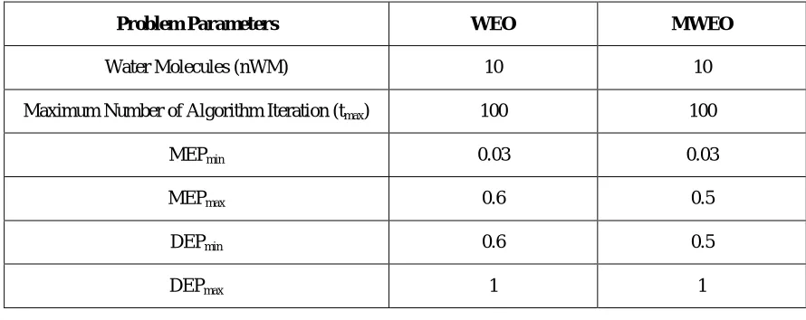
The application of WEO algorithm is extended to solve the combined UC and Emission problem in 10-unit system with 10% spinning reserve and without considering ramp rate constraint. The WEO algorithm parameters for all test systems are shown in
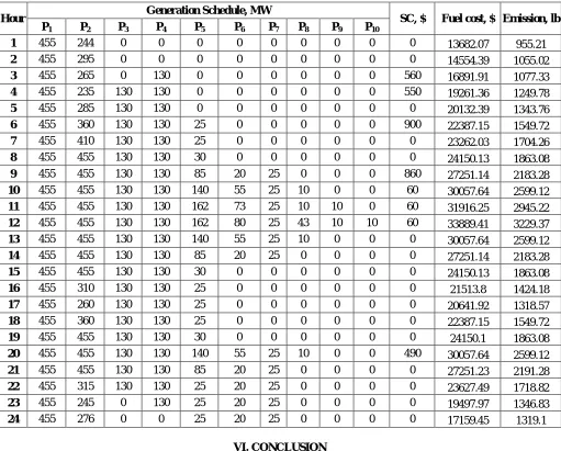
Table 5.1. The test system particulars are adopted from [27]. Table 5.2 presents the 24h committed schedule for the 10-unit case and
Table 5.3 shows the comparison of the proposed method to other popular method. The dispatch of each generating unit shows that the generating capacity limit constraint as well as minimum up and down constraints is satisfied. As comparison shows, the best total
cost obtained using MWEO is $ 1111845.12 and emission of 43732.15 which is lesser than compared to RCGWO [27].
TABLE 5.1 PROBLEM PARAMETERS OF WEO ALGORITHM
Problem Parameters WEO MWEO
Water Molecules (nWM) 10 10
Maximum Number of Algorithm Iteration (tmax) 100 100
MEPmin 0.03 0.03
MEPmax 0.6 0.5
DEPmin 0.6 0.5
DEPmax 1 1
TABLE 5.3 COMPARISON RESULTS OF TEST SYSTEM 16
Method Total Cost $ Emission, lb
RCGWO 1111956 43732.98
WEO 1111845.35 43732.82
TABLE 5.2 TEST RESULTS OF 10-UNIT SYSTEM FOR COMBINED UC AND EMISSION MINIMIZATION
Hour Generation Schedule, MW SC, $ Fuel cost, $ Emission, lb
P1 P2 P3 P4 P5 P6 P7 P8 P9 P10
1 455 244 0 0 0 0 0 0 0 0 0 13682.07 955.21 2 455 295 0 0 0 0 0 0 0 0 0 14554.39 1055.02 3 455 265 0 130 0 0 0 0 0 0 560 16891.91 1077.33 4 455 235 130 130 0 0 0 0 0 0 550 19261.36 1249.78 5 455 285 130 130 0 0 0 0 0 0 0 20132.39 1343.76 6 455 360 130 130 25 0 0 0 0 0 900 22387.15 1549.72 7 455 410 130 130 25 0 0 0 0 0 0 23262.03 1704.26 8 455 455 130 130 30 0 0 0 0 0 0 24150.13 1863.08 9 455 455 130 130 85 20 25 0 0 0 860 27251.14 2183.28 10 455 455 130 130 140 55 25 10 0 0 60 30057.64 2599.12 11 455 455 130 130 162 73 25 10 10 0 60 31916.25 2945.22 12 455 455 130 130 162 80 25 43 10 10 60 33889.41 3229.37 13 455 455 130 130 140 55 25 10 0 0 0 30057.64 2599.12 14 455 455 130 130 85 20 25 0 0 0 0 27251.14 2183.28 15 455 455 130 130 30 0 0 0 0 0 0 24150.13 1863.08 16 455 310 130 130 25 0 0 0 0 0 0 21513.8 1424.18 17 455 260 130 130 25 0 0 0 0 0 0 20641.92 1318.57 18 455 360 130 130 25 0 0 0 0 0 0 22387.15 1549.72 19 455 455 130 130 30 0 0 0 0 0 0 24150.1 1863.08 20 455 455 130 130 140 55 25 10 0 0 490 30057.64 2599.12 21 455 455 130 130 85 20 25 0 0 0 0 27251.23 2191.28 22 455 315 130 130 25 20 25 0 0 0 0 23627.49 1718.82 23 455 245 0 130 25 20 25 0 0 0 0 19497.97 1346.83 24 455 276 0 0 25 20 25 0 0 0 0 17159.45 1319.1
VI. CONCLUSION
REFERENCES
1. Wood A. J, and Wollenberg B. F, (1996), Power generation, operation and control, Second Edition, John Wiley and Sons, New York
2. Virmani S, Adrian E. C, and Imhif, K, (1989), Implementation of Lagrangian based unit commitment problem, IEEE Transaction on Power
System, Vol. 4, No. 4, pp. 1373–1380.
3. Ongsakul W, and Petcharaks N, (2004), Unit commitment by enhanced adaptive Lagrangian relaxation, IEEE Transaction on Power System,
Vol. 19, No. 1, pp. 620–628.
4. Chandram K, Subrahmanam N, and Sydulu M, (2011), Unit commitment by improved pre-prepared power demand table and Muller method,
Electric Power and Energy System, Vol. 33, pp. 106–114.
5. Hobbs W. J, Hermon G, Warner S, and G. B. Sheble, (1988), An enhanced dynamic programming approach for unit commitment, IEEE
Transaction on Power System, Vol. 3, No. 3, pp. 1201-1205.
6. Marian Marcoveccio G, Augusto Novals Q, and Ignacio Grossmann E, (2014), Deterministic optimization of the thermal unit commitment
problem: a branch and cut search, Computers and Chemical Engineering, Vol. 67, pp. 53–68.
7. Han D, Jian J, and Yang L, (2014), Outer approximation and outer-inner approximation approaches for unit commitment problem, IEEE
Transaction on Power System, Vol. 29, No. 2, pp. 505–513.
8. Roy P. K, (2013), Solution to the unit commitment problem using gravitational search algorithm, Electrical Power and Energy Systems, Vol. 53,
pp. 85–94.
9. Burns R. M, and Gibson C. A, (1975), Optimization of priority lists for a unit commitment program, IEEE PES proceedings, Vol. 75, pp.
453-461.
10. Patra S, Goswami S. K, and Goswami B, (2008), Differential evolution algorithm for solving unit commitment with ramp constraints,
Electrical Power and Components System, Vol. 36, No. 8, pp. 771–787.
11. Kazarlis S. A, Bakirtzis A. G, and Petridis V, (1996), A genetic algorithm solution to the unit commitment problem, IEEE Transaction on
Power System, Vol. 11, No. 1, pp. 83–92.
12. Juste K. A, Kita H, and Tanaka E, (1999), An evolutionary programming solution to the unit commitment problem, IEEE Transaction on
Power System, Vol. 14, pp. 1452–1459.
13. Zhuang F, and Galiana F. D, (1990), Unit commitment by simulated annealing, IEEE Transaction on Power System, Vol. 5, pp. 311–317.
14. Ebrahimi J, Hosseinian S. H, and Gevorg B, (2011), Unit commitment problem solution using shuffled frog leaping algorithm, IEEE
Transaction on Power System, Vol. 26, No. 2, pp. 573–581.
15. Roy P. K, (2013), Solution to the unit commitment problem using gravitational search algorithm, Electrical Power and Energy Systems, Vol. 53,
pp. 85–94.
16. Roy P. K, and Sarkar R, (2014), Solution of unit commitment problem using quasi-oppositional teaching learning based algorithm, Electrical
Power and Energy System, pp. 96–106.
17. Eslamian M, Hosseinian S, and Vahidi B, (2009), Bacterial foraging based solution to the unit commitment problem, IEEE Transaction on
Power System, Vol. 24, No. 3, pp. 1478–1488.
18. Saber A. Y, Senjyu T, and Miyagi T, (2006), Fuzzy Unit commitment scheduling using absolute stochastic simulated annealing, IEEE
Transaction on Power System, Vol. 21, No. 2, pp. 955–964.
19. Damousis I. G, Bakirtzis A. G, and Dokopoulos P. S, (2004), A solution to the unit commitment problem using integer coded genetic
algorithm, IEEE Transaction on Power System, pp. 1165–1172.
20. Zhao B, Guo C. X, and Bai B. R, (2006), An improved particle swarm optimization algorithm for unit commitment, Electric Power and Energy
System, Vol. 28, No. 7, pp. 482–490.
21. Cheng C. P, Liu C. W, and Liu G. C, (2000), Unit commitment by Lagrangian relaxation and genetic algorithms, IEEE Transaction on Power
System, Vol. 15, No. 2, pp. 707–714.
22. Kumar N, Panigrahi B. K, Bhim Singh, (2016), A solution to the ramp rate and prohibited operating zone constrained unit commitment by
GHS-JGT evolutionary algorithm, Electrical power and Energy system, Vol. 81, pp. 193-203.
23. Lau T. W, Chung C. Y, and Wong K. P, (2009), Quantum inspired evolutionary algorithm approach for unit commitment, IEEE Transaction
on Power System, Vol. 24, No. 3, pp. 1503–1512.
24. Jeong Y. W, Park J. B, and Jang S. H, (2010), A new quantum inspired binary PSO: application to unit commitment problems for power
systems, IEEE Transaction on Power System, Vol. 25, No. 3, pp. 1486–1495.
25. Quan R, Jian J, and Yang L, (2015), An improved priority list and neighborhood search method for unit commitment, Electric Power and Energy System, Vol. 67, pp. 278–285.
26. Kaveh A, and Bakhshpoori T, (2016), Water Evaporation Optimization: A novel physically inspired optimization algorithm, Computer and
Structures, Vol. 167, pp. 69-85.
27. Rameshkumar J, Ganesan S, Abirami M, and Subramanian S, (2015), cost, emission and reserve pondered pre dispatch of thermal
generating units coordinated with real coded grew wolf optimization, IET generation Transmission and Distribution, Vol. 45, pp. 1-14.