Integrating Genetic Linkage Maps With Pachytene
Chromosome Structure in Maize
Lorinda K. Anderson,*
,1Naser Salameh,
†Hank W. Bass,
‡Lisa C. Harper,
§W. Z. Cande,
§Gerd Weber
†and Stephen M. Stack*
*Department of Biology, Colorado State University, Fort Collins, Colorado 80523,†Department of Plant Breeding and Biotechnology,
University of Hohenheim, D-70593 Stuttgart, Germany,‡Department of Biological Science, Florida State University,
Tallahassee, Florida 32306 and§Department of Molecular and Cell Biology,
University of California, Berkeley, California 94720 Manuscript received November 4, 2003 Accepted for publication January 9, 2004
ABSTRACT
Genetic linkage maps reveal the order of markers based on the frequency of recombination between markers during meiosis. Because the rate of recombination varies along chromosomes, it has been difficult to relate linkage maps to chromosome structure. Here we use cytological maps of crossing over based on recombination nodules (RNs) to predict the physical position of genetic markers on each of the 10 chromosomes of maize. This is possible because (1) all 10 maize chromosomes can be individually identified from spreads of synaptonemal complexes, (2) each RN corresponds to one crossover, and (3) the frequency of RNs on defined chromosomal segments can be converted to centimorgan values. We tested our predic-tions for chromosome 9 using seven genetically mapped, single-copy markers that were independently mapped on pachytene chromosomes usingin situhybridization. The correlation between predicted and observed locations was very strong (r2⫽0.996), indicating a virtual 1:1 correspondence. Thus, this new,
high-resolution, cytogenetic map enables one to predict the chromosomal location of any genetically mapped marker in maize with a high degree of accuracy. This novel approach can be applied to other organisms as well.
I
NTEGRATING genetic linkage maps with chromo- organized meiotic chromosomes. This is an importantpoint because the observed location of a gene on a some structure has been an important objective ever
since it was demonstrated that genes occur in a fixed chromosome (relative to the centromere) can be
differ-ent on mitotic compared to meiotic chromosomes, as
order on chromosomes (Sutton1903;Bridges1916).
demonstrated by Froenicke et al. (2002) for mouse
Linkage maps are defined by the percentage of
recombi-chromosomes. Related observations indicate that differ-nation between markers [as expressed in centimorgans
ences in mitotic and meiotic chromosomes may affect (cM)] and reveal the linear order of markers. However,
the relative cytological distance between markers in they do not contain information on the actual physical
plants as well (Stack1984). In this regard, Drosophila
distance between markers, whether that distance is
ex-melanogasterhas the best integration of cytological (chro-pressed as a cytological length (positions on
chromo-mosome), genetic (recombination), and physical (DNA somes) or as a physical length (number of DNA base
sequence) aspects of the genome, but this integration pairs). This is because crossing over is not evenly
distrib-is based on somatic polytene chromosomes (http://fly uted along chromosomes. Crossing over is suppressed
base.bio.indiana.edu/), not on meiotic chromosomes in heterochromatin and centromeres, and crossing over
where crossing over actually occurs. For these reasons, is variable even in euchromatin where most crossing
the position of individual genes along meiotic
chromo-over occurs (Sherman and Stack 1995; Harper and
somes and the relation of gene position to meiotic re-Cande2000;Andersonet al.2003). As a result, linkage
combination are understood only in general terms for maps cannot be simply overlaid on chromosomes to
most organisms. determine the physical position of genes. Even detailed
Here we relate linkage maps to meiotic chromosome information on the linear order of genes from a
com-structure in maize by using the distribution of cytologi-plete genome sequence cannot bridge the gap between
cally visible markers of crossing over called late recombi-linkage maps and chromosomes because DNA (as well
nation nodules (RNs) on individually identified pachy-as crossing over) is not evenly distributed along specially
tene chromosomes (Anderson et al. 2003). RNs are
proteinaceous, multicomponent, ellipsoidsⵑ100 nm in
diameter that are found in the central region of
synapto-1Corresponding author:Department of Biology, Colorado State
Uni-nemal complexes (SCs) between homologous
chromo-versity, Fort Collins, Colorado 80523.
E-mail: [email protected] somes (bivalents) at pachytene (ZicklerandKleckner
a total of 193 SCs identified as SC2 would be equal to a map 1999). Evidence that RNs mark crossover sites include
length of (7 RNs⫻50 cM/RN)⫼193 SCs⫽1.81 cM. This the close correspondence between the frequency and
operation was performed for every 0.2-m segment on each
distribution of RNs compared to chiasmata (e.g.,Car- of the 10 maize SCs. Cumulative centimorgan maps were
con-penter 1979; Anderson et al. 2003), the presence of structed for each bivalent by adding the centimorgan values for adjacent intervals along the length of the SC (starting
an essential crossover protein (MLH1p) in RNs (Moens
from the tip of the short arm). The centimorgan RN (RN-et al.2002), and the presence of MLH1p/RNs at chiasma
cM) maps for all maize chromosomes are available at http://
sites (MarconandMoens 2003). Because RNs can be
www.maizegdb.org.
observed only by electron microscopy of SCs in elongate Adjusting the UMC98 map to fit the cumulative RN-cM map:
pachytene bivalents, RNs represent the highest resolu- Because the UMC98 maize linkage maps are almost twice as
long as the RN-cM maps (Andersonet al.2003), it was neces-tion markers available for determining the
chromo-sary to adjust theUMC98marker positions proportionally to somal location of crossing over. Each RN represents
fit onto the RN-cM map. The markers were converted using one crossover (equivalent to 50 cM on a linkage map),
the following formulas whereAis centimorgan length of the
so the frequency and distribution of RNs can be used short arm, B is centimorgan length of the long arm, C is
to prepare a detailed map of recombination along the centimorgan position of the centromere measured from the
tip of the short arm,ais centimorgan position of a marker physical length of each of the 10 pachytene
chromo-in the short arm, andbis centimorgan position of a marker
somes/SCs in maize (Andersonet al.2003). Because RN
in the long arm. Subscripts UMC98 and RN indicate origin maps relate the amount of recombination to cytological
from the UMC98 and RN-cM maps, respectively. For short
position along pachytene chromosomes and linkage arm markers (a
UMC98/AUMC98)⫻ARN⫽aRN. For long arm markers
maps report the amount of recombination relative to {[(bUMC98⫺CUMC98)/BUMC98]⫻BRN}⫹CRN⫽bRN. The predicted
physical position of a marker in the short or long arm of a genes or other markers, it is now possible to combine
pachytene chromosome (SC position) was then determined these two approaches to directly relate genetically
by finding the 0.2-m interval on the cumulative centimorgan mapped markers to cytological position. Here, we use
RN map, which includes the adjusted marker position. All
our RN maps to predict the cytological location of se- features used to calculate the centimorgan and SC positions
lected linkage map markers on each maize chromo- for all 90 core bin markers are in theappendix.
In situ hybridization:The bacterial artificial chromosome
some. The predicted locations of seven markers on
chro-(BAC) 60.j16(encompassing the marker crcbr58rwith a
ge-mosome 9 were tested usingin situhybridization (ISH)
netic map position of 96.1 cM on chromosome 9) from Du-of single-copy DNA sequences. The predicted and
ob-pont was localized using procedures described bySadderand
served locations of the markers on chromosome/SC 9 Weber(2002). Data concerning all other markers used here
were highly correlated, indicating a virtual 1:1 match. have been published (Shen et al.1987; Sadder et al.2000;
KoumbarisandBass2003). From this we conclude that high-resolution RN maps
can be used to accurately predict the cytological location of any genetically mapped marker.
RESULTS
Predicting the cytological position of genetically
MATERIALS AND METHODS mapped markers: The frequency of RNs in each 0.2-m interval for each of the 10 maize pachytene SCs was Preparing recombination maps on pachytene bivalents:
Us-ing SC spreads from the inbred strain KYS, the locations of converted to a centimorgan value and then summed centromeres and RNs were measured on each of the 10 maize along the length of each SC to produce a cumulative pachytene bivalents (Andersonet al.2003). Briefly, a standard centimorgan map based on RNs (RN-cM map) for each SC karyotype was developed in which each SC was identified
bivalent (Figure 1, SCs 1–10). These maps are based by relative length and arm ratio. This SC karyotype is very
on the positions of 4267 RNs from 2080 individually similar to karyotypes developed from pachytene chromosome
squashes. Using the SC karyotype and an average measured identified SCs (Andersonet al. 2003). Although each length of 331 m for a complete set of SCs, the average bivalent has a unique pattern of RNs (and a correspond-absolute length of each SC arm was established to the nearest ingly unique centimorgan map), all 10 SCs show the 0.1 m. The locations of RNs on identified SCs were
deter-same general trends with high levels of crossing over mined as percentages of the arm length from the centromeres,
distally on each arm and reduced crossing over proxi-and these values were then converted to absolute positions in
micrometers on each of the 10 standardized SCs. The locations mally (near the centromeres). The number of centi-of 4267 RNs on 2080 individually identified SCs from 47 plants morgans per 0.2-m interval was typically 0 near the were compiled in 0.2-m intervals (Andersonet al.2003). SC centromeres of all SCs while the maximum centimorgan lengths that were not evenly divisible by 2 (SCs 3, 5, 6, 8,
value for a single distal interval ranged from 2.56 cM 9, and 10) have one larger 0.3-m SC segment nearest the
for SC9 to 4.85 cM for SC4. centromere in either the short or the long arm. One RN
represents a crossover between two homologous, nonsister Once the centimorgan value of each 0.2-m interval chromatids, which yields two recombinant and two parental is determined, it is possible to relate a specific genetically chromatids for a recombination frequency of 50% (or 50 cM). mapped marker to a particular position on a chromo-On this basis, RN frequency was converted to centimorgans
some. Certain markers (called core bin markers) were by multiplying the number of RNs in each 0.2-m SC segment
selected byDaviset al.(1999) to enable different
link-by 50 cM and then dividing link-by the number of SCs observed.
to one another. Core bin markers are separated byⵑ20 phy. Nevertheless, the ISH procedure is essentially the same, and autoradiography yields results that are com-cM on each chromosome. Because of their utility and
more or less even genetic spacing, we chose to map the parable to fluorescencein situhybridization (FISH). In
addition, the observed ISH position of the wx1 locus
location of these markers on the SCs. A number of
different linkage maps are available for maize, but we close to the centromere in the short arm of chromosome
9 is consistent with linkage and comparative grass ge-used the UMC98 linkage map here because this map is
finished, has many markers that are shared with other nome analyses (Ramakrishnaet al.2002). The
differ-ences between the predicted and observed chromo-linkage maps, and includes the genetic locations of
cen-tromeres (http://www.maizegdb.org;Daviset al.1999). somal location of the sequences ranged from 0.02m
(wx1) to 0.84 m (csu54b; Table 1; Figure 2). These
For each bivalent, the UMC98 linkage map is longer,
i.e., more total map units, than the cumulative centi- values represent differences ofⵑ0.1 and 3.3%, respec-tively, of the total length of SC9. When the observed
morgan RN map (Davis et al. 1999; Anderson et al.
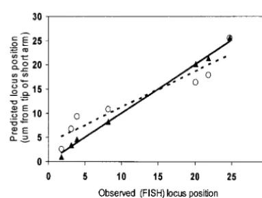
2003), so the centimorgan value of each core bin marker and predicted locations of the seven markers are plotted
(Figure 3), the regression equation (y⫽1.01x⫺0.04,
was adjusted proportionally on an arm-by-arm basis to
fit onto the corresponding RN map. The adjusted centi- r2⫽0.996) indicates a virtual 1:1 correspondence.
Simi-lar plots using the IBM2 neighbors frame 9 map (http:// morgan value of each core bin marker was placed onto
the RN-cM map to predict the physical location of each www.maizegdb.org;Leeet al.2002) also gave an
excel-lent correspondence between observed and predicted marker on the appropriate pachytene chromosome
(Figure 1; SCs 1–10). marker locations (y ⫽ 0.98x ⫹ 0.62, r2 ⫽ 0.996). In
comparison, the correspondence between the observed Variability in crossover rates along maize
chromo-somes is demonstrated by the differences in the spacing ISH positions of the markers with the predicted
posi-tions based simply on their relative (%) posiposi-tions in the of the predicted location of core bin markers. Markers
are closer to one another in distal regions that have UMC98 linkage map is not as good (r2⫽ 0.90), and a
number of points are clearly off the regression line high levels of crossing over than in proximal regions
with low levels of crossing over. In some cases, the mark- (Figure 3). It appears that the RN-cM map helps to
fine-tune the predicted location of the markers because it ers are spaced more or less evenly at the distal ends of
arms (e.g., 1S, 2L, 6L, and 8L), while in other cases, the corrects for differences in recombination rate along the
length of chromosome 9. spacing between markers is more variable (e.g., 3S, 3L,
and 4L). The spacing variations for core bin markers Predicted genetic positions of centromeres
corre-spond well to other estimates of centromere genetic
on SCs 3 and 4 are due to both differences in spacing
between the markers in the UMC98 maps (with separa- position:It is possible that there are substantial
differ-ences in the centromere locations estimated by genetic tions between markers of 5–12 cM rather than the
typi-cal 20 cM) and differences in recombination (RN) fre- maps and those observed on SCs (where centromeres
are directly visible). To test this, we compared the ge-quency along the SCs.
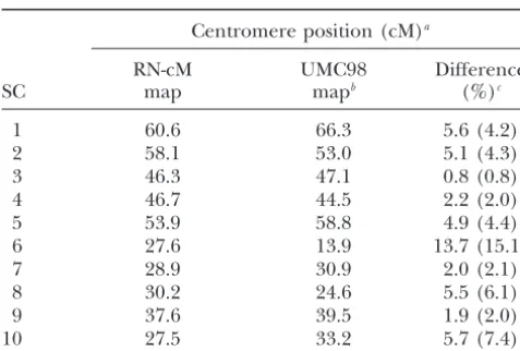
Predicted cytological locations of genetic markers are netic centromere positions from the UMC98 maps with those shown on our RN-cM maps (Table 2). The
corre-almost identical to cytological positions determined by
in situhybridization:Pachytene chromosome identifica- spondence was good (r2⫽0.84) with the largest differ-ence noted for chromosome 6 that carries the nucleolar-tion is based on squash preparanucleolar-tions in which each
bivalent can be identified by its characteristic arm ratio organizing region on the short arm. With the exception
of chromosome 6, the differences in centromere
posi-and relative length within the set (McClintock et al.
1981). These same characters can be used to accurately tion are probably not great enough to have a large effect
on the predicted cytological position of markers. identify maize pachytene chromosomes in squash
prepa-rations for both ISH and SC spreads (Shenet al.1987;
SadderandWeber2002;Andersonet al.2003;
Koum-DISCUSSION
barisandBass2003). Thus, the features of pachytene
chromosome structure used for identification do not Integration of RN-cM maps with genetic linkage maps
to predict the cytological location of markers:While a change with different preparative procedures, and
marker locations can be reliably compared whether RN linkage map represents the linear order of markers and
the frequency of recombination between markers on a maps on SCs or ISH markers on pachytene
chromo-somes are used. chromosome, usually this map is related to the physical
structure of the chromosome in only a general way. One We tested the predicted positions of markers on
chro-mosome 9 using seven different single-copy sequences reason for this is that the rate of recombination varies
in different parts of the genome (e.g., Sherman and
that have been independently mapped using ISH (Shen
et al.1987;Sadderet al.2000;SadderandWeber2002; Stack1995;Sharopovaet al.2002). Thus, two markers located in a chromosomal region with a high rate of KoumbarisandBass2003). Each of these studies used
fluorescent detection of markers except Shen et al. crossing over may be physically close together but
sepa-rated by a comparatively large linkage map distance,
autoradiogra-TABLE 1
Predicted and observed locations for seven markers on maize SC/chromosome 9
Location of marker on SC (micrometers from tip Centimorgan position of short arm)
Difference (m) in Symbol in UMC98 Adjusted for Predicted from Observed by marker positions Marker Figure 2a map RN mapb RN map ISHc (% of total SC length)
umc109 1 15.5 9.1 1.0 1.8 0.8 (3.3)
bz1 2 39.3 23.1 3.4 3.1 0.4 (1.4)
umc105a a 54.7 32.1 4.6 3.9 0.7 (2.7)
wx1 3 63.7 37.4 8.2 8.2 0.02 (0.1)
60.j16 b 96.1 58.1 20.1 20.1 0.04 (0.2)
csu145a c 105.4 64.0 21.3 21.8 0.5 (2.0)
csu54b 8 150.4 92.7 25.5 24.7 0.8 (3.3)
aCore bin markers are indicated by numerals while other markers are indicated by letters. bSeematerials and methodsfor calculation details.
cCalculated from ISH marker position as a percentage of arm length.
and vice versa for markers located in regions with low the mapping is not influenced by inherent differences
in the relative degree of chromosome condensation of
rates of crossing over (e.g.,Gillet al.1996;Harperand
Cande 2000; Ku¨ nzel et al. 2000; Sadder and Weber euchromatin and heterochromatin. In addition, al-though maize chromosomes continue to contract
dur-2002;Koumbaris andBass2003).
RN-cM maps provide an opportunity to bridge the ing pachytene (Gillies1973), the contraction is
consis-tent among all the chromosomes in a set and does not gap between linkage maps and meiotic chromosome
structure. RNs are high-resolution markers of crossing substantially affect arm ratio or relative length (
Ander-sonet al.2003). The difficulty of single-copy ISH
map-over on pachytene chromosomes (Andersonet al.2003)
that can be used to directly convert linkage map position ping in maize limited the number of markers that were
available to compare with our RN-cM predictions. Nev-to chromosome position on the basis of crossover
fre-quency. We used this property to predict the location ertheless, for chromosome 9, we were able to compare
the positions of seven single-copy ISH markers with our of core bin markers on each of the 10 bivalents of maize.
Currently, the best method available for testing our predictions from the RN-cM map. This comparison
re-vealed a virtual 1:1 correspondence (Figures 2 and 3). predictions in maize is by comparisons with single-copy
DNA markers that have been localized to pachytene This excellent correspondence indicates that (1)
pachy-tene chromosome structure is not changed substantially chromosomes using ISH. Since RNs and ISH markers
are both mapped on pachytene chromosomes (SCs),
Figure3.—Plots comparing observed and predicted posi-tions of sevenUMC98markers on maize chromosome 9. Trian-Figure2.—Comparison of the predicted (solid circles on
cumulative centimorgan curve and drop-down lines) and ob- gles are from the RN-cM map. Open circles are from the UMC98 map with each marker expressed as a percentage of served (by ISH, arrows) location of genetically mapped
mark-ers on maize chromosome 9 (drawn in bottom part of graph). the total chromosome centimorgan map length. The pre-dictive power of the RN map comparison (y⫽1.01x⫺0.04, The numbers correspond to core bin markers and the letters
correspond to other genetically mapped markers that have r2⫽0.996, solid line) is better than that of the UMC98 map
comparison (y⫽0.71x⫹3.88,r2⫽0.900, broken line).
TABLE 2 ping, which is higher resolution and not compromised by nonhomologous synapsis. In addition, RN-cM maps Comparison of centromere positions for
supply a valuable comparison for cytological mapping UMC98 and RN maps
using radiation hybrids (Riera-Lizarazuet al.2000).
Two other studies, one in tomato and one in mouse, Centromere position (cM)a
have combined FISH of genetically mapped markers RN-cM UMC98 Difference
with cytological crossover maps based on RNs and
SC map mapb (%)c
MLH1 fluorescent foci, respectively (Peterson et al.
1 60.6 66.3 5.6 (4.2) 1999;Froenickeet al.2002). Unfortunately,Peterson 2 58.1 53.0 5.1 (4.3) et al.(1999) were unable to directly compare the
molec-3 46.3 47.1 0.8 (0.8)
ular and cytological maps for three markers on
chromo-4 46.7 44.5 2.2 (2.0)
some 11 because the order of the markers was different
5 53.9 58.8 4.9 (4.4)
in the two maps, perhaps indicating a small
re-6 27.6 13.9 13.7 (15.1)
arrangement in one of the tomato populations used for
7 28.9 30.9 2.0 (2.1)
8 30.2 24.6 5.5 (6.1) mapping. On the other hand,Froenickeet al.(2002) 9 37.6 39.5 1.9 (2.0) found a good correspondence between the position ex-10 27.5 33.2 5.7 (7.4) pected from the MLH1 map and the position observed
by FISH for five genetically mapped markers on two aFrom end of short arm.
bAdjusted to RN-cM map. mouse chromosomes. However, because each of the cPercentage difference values are the same when using
two chromosomes had only two or three markers for UMC98 map. comparison,Froenicke et al. (2002) were not able to
rigorously test the correspondence between the ex-pected and observed positions.
by the different procedures used for ISH and for prepar- Correspondence between RN-cM maps and linkage
ing SC spreads and (2) RN-cM maps and linkage maps maps: The correspondence between the marker
posi-are closely related (even though the maps differ in over- tions predicted by the RN-cM map and those observed
all length). Most importantly, these results demonstrate by ISH on maize chromosome 9 is particularly striking
that by using these RN-cM maps it is possible to predict when one considers the variables involved in the
com-the cytological position of any genetic marker in maize parison. For example, the observed ISH marker
loca-on the basis of its map positiloca-on relative to the UMC98 tions were from four different groups using somewhat
linkage map. different methods. The good correspondence indicates
While the correspondence between the predicted and that our RN-cM map is useful in positioning markers
observed locations of markers for chromosome 9 is very regardless of the source of the ISH data. Another
impor-good, it should be kept in mind that the RN-cM map tant difference is that the UMC98 linkage map [as well
is compiled from the positions of 434 RNs on 234 SCs as other maize linkage maps (Andersonet al.2003)] is
placed onto an average SC 9 and the ISH maps are about twice as long as the RN-cM map. The reason(s)
based on the average position of ISH markers similarly for the discrepancies in map lengths is unclear, but
placed onto an average pachytene chromosome 9. Nev- there are a number of differences in the procedures and
ertheless, our results demonstrate the utility of this ap- populations used to generate the maps. The UMC98
proach in determining the location of specific markers linkage map is based on analysis of an immortal F2
popu-on maize chromosomes. In additipopu-on, the locatipopu-on of lation of a genetic cross between two inbred lines (Tx303
any marker can be individually estimated, and it is not and CO159;Daviset al.1999) and includes both male
necessary to interpolate the position of a marker of and female recombination. In comparison, the RN-cM
interest on the basis of its proximity to an anchored map is based on cytological observations of male cells
marker on a chromosome. Such interpolations can be from a single inbred line, KYS. Several investigators have
seriously affected by variation in recombination fre- reported differences in recombination frequency
re-quency along the length of the chromosomes. Because lated to such variables as environmental conditions,
dif-recombination variation is directly charted by RN-cM ferent inbred lines, and different crosses in maize (
Wil-maps, better estimates of marker position are possible. liamset al.1995;Andersonet al.2003). Other potential
To date, cytological and molecular maps in maize contributors to the differences are the type of computer
have been merged primarily using A-A and B-A translo- program used to assemble the molecular maps and the
cations (WeberandHelentjaris1989;Beckett1991). value chosen in the computer program to indicate the
While genetic mapping of translocation breakpoints can strength of interference (see discussion by King et al.
be precise (Beckett1991), cytological mapping is often 2002). Another possibility is that the RN-cM map is too
complicated by nonhomologous synapsis in the vicinity small because some RNs are lost at random. However,
of the breaks that obscures the true breakpoints (Long- this is unlikely because there should be many more SCs
ley 1963). RN-cM maps provide a complementary ap- with no RNs than are observed (Andersonet al.2003).
map-between predicted and observed marker locations on chromosome 9, the differences between the RN-cM and linkage maps appear to be distributed proportionally along the entire length of the chromosome, at least at the resolution examined. These results also indicate that the RN-cM and the UMC98 maps are closely related measures of crossing over.
The presence of mapped centromeres in the UMC98 linkage map aided the positioning of markers on the chromosomes. This is because the low frequency of crossing over and the rather flat cumulative centi-morgan map in pericentromeric regions means that resolution around centromeres is low. Indeed, when we ignored the position of the centromeres and mapped the predicted location of the seven markers on chromo-some 9 from the tip of the short arm by simply multi-plying their UMC map positions by the ratio of the
RN-cM map length to the UMC98 map length,wx1mapped
to the long arm (11.9m) rather than to the short arm
(8.2 m) where it has been located by ISH, linkage, and comparative genome analyses. In contrast, four of the other six more-distal markers changed position only
slightly (0.2–0.4m or 0.7–1.4% of the total length of
SC 9). Thus, predicting the location of markers as a function of their distance from the centromere is partic-ularly important for markers around centromeres.
Integration of the RN-cM and linkage maps reveals that most of the linkage map (including core bin mark-ers and genes) is located distally (Figures 1 and 4). This suggestion is also supported by the observation that
genes are hot spots for recombination (Civardiet al.
1994;Schnableet al.1998;Fuet al.2001, 2002;Yaoet
al.2002). A similar clustering of genes in distal regions
of chromosomes has been reported for other cereal
grains (e.g.,Gillet al.1996).
Resolution of the RN-cM map:The resolution of the RN-cM map is based on the 1671 0.2-m SC segments that were used for mapping. Segments this size corre-spond to 0.4% (SC1) to 0.9% (SC10) of pachytene chro-mosome length. The resolution of the maize RN-cM map in terms of DNA amount can be calculated to be
ⵑ1.6 Mbp of DNA per 0.2-m segment (2675 Mbp per
1C DNA⫼1671 segments;Bennettet al.2000).
How-ever, this calculation assumes that the DNA is evenly distributed along the length of each chromosome. In tomato, heterochromatic regions of pachytene chromo-somes contain about six times more DNA per
microme-ter of SC than do euchromatic regions (Petersonet al.
1996). While the heterochromatin of maize (aside from knobs) is not as prominent as that of tomato, the amount of DNA per SC length in the more heterochro-matic proximal segments of maize pachytene
chromo-somes (Carlson1988) is undoubtedly higher than the
average value of 1.6 Mbp per segment, while that of the more distal, gene-rich, euchromatic regions is conse-quently lower than the average value. Thus, the
resolu-Figure 4. — Integrated cytogenetic map (in micrometers) of all 10 maize chromosomes/SCs with the p redicted position (based on the RN-cM map for each chromosome) of core bin m arkers from the UMC98 linkage map. Core b in markers are rather evenly spaced genetically but not physically on the chromosomes. C, centrom ere.
ex-Florida State University Research Foundation (to H.B.); and
Eiselens-pected from radiation hybrids (Riera-Lizarazu et al.
tiftung, Ulm, Germany (to G.W.).
2000).
In terms of centimorgans, the resolution of the
RN-cM map can be calculated to averageⵑ0.62 cM per
0.2-LITERATURE CITED m SC segment (1030 cM⫼1671 segments;Anderson
Anderson, L. K., G. G. Doyle, B. Brigham, J. Carter, K. D. Hooker
et al. 2003). This calculation is an oversimplification
et al., 2003 High resolution crossover maps for each bivalent of
since RN frequency varies along maize pachytene
chro-Zea maysusing recombination nodules. Genetics165:849–865.
mosomes. For example, many proximal segments have Beckett, J. B., 1991 Cytogenetic, genetic and plant breeding
appli-cations of B-A transloappli-cations in maize, pp. 493–529 inChromosome
essentially 0 cM per segment while more distal segments
Engineering in Plants, Pt. A, edited by T.Tsuchiya and P. K.
(specifically, the most distal 3m of each arm) average
Gupta. Royal Botanic Gardens, Kew, UK.
1.44 cM per 0.2 m segment. Thus, distal regions of Bennett, M. D., A. V. CoxandI. J. Leitch, 2000 Angiosperm DNA
C-values database (http://www.rbgkew.org.uk/cval/homepage.
SCs where most of the genes are located tend to have
html).
both less DNA per unit SC length and at least a twofold
Bridges, C. B., 1916 Nondisjunction as proof of the chromosome
higher crossover frequency than the genome as a whole. theory of heredity. Genetics1:1–52.
Carlson, W. R., 1988 The cytogenetics of corn, pp. 259–331 inCorn
Conclusion: Currently, integration of linkage maps
and Corn Improvement, edited by G. F.Spragueand J. W.Dudley.
with chromosome structure relies heavily on mapping Crop Science Society, Madison, WI.
multiple single-copy FISH markers, often on mitotic Carpenter, A. T. C., 1979 Synaptonemal complex and
recombina-tion nodules in wild typeDrosophila melanogasterfemales. Genetics
chromosomes (e.g., humans, Korenberg et al. 1999)
92:511–541.
with more recent mapping using pachytene chromo- Cheng, Z., G. G. Presting, C. R. Buell, R. A. WingandJ. Jiang,
somes (e.g., rice chromosome 10, Cheng et al. 2001; 2001 High-resolution pachytene chromosome mapping of
bac-terial artificial chromosomes anchored by genetic markers reveals
maize chromosome 9, Sadder and Weber 2002;
the centromere location and the distribution of genetic
recombi-KoumbarisandBass2003). Unfortunately, single-copy nation along chromosome 10 of rice. Genetics157:1749–1757.
FISH is particularly difficult in species such as maize Civardi, L., Y. Xia, K. Edwards, P. S. SchnableandB. J. Nikolau,
1994 The relationship between genetic and physical distances
that have many duplications and repetitive sequences
in the clonedal-sh2interval ofZea maysL. genome. Proc. Natl.
(SadderandWeber2002). Here we demonstrate that Acad. Sci. USA91:8268–8272.
the cytological crossover (RN-cM) map for maize SC 9 Davis, G. L., M. D.McMullen, C.Baysdorfer, T.Musket, D.Grant
et al., 1999 A maize map standard with sequences core markers,
can be used to integrate accurately genetically mapped
grass genome reference points and 932 expressed sequence
loci with the structure of the pachytene chromosome. tagged sites (ESTs) in a 1736-locus map. Genetics152:1137–1172.
Froenicke, L., L. K. Anderson, J. WeinbergandT. Ashley, 2002
On the basis of this result, it is likely that the RN-cM
Male mouse recombination maps for each autosome identified
maps will be equally useful in predicting the location of
by chromosome painting. Am. J. Hum. Genet.71:1353–1368.
genetically mapped markers on the other nine bivalents. Fu, H., W. Park, X. Yan, Z. Zheng, B. Shenet al., 2001 The highly
recombinogenicbzlocus lies in an unusually gene-rich region of
Our predictions for the locations of core bin markers
the maize genome. Proc. Natl. Acad. Sci. USA98:8903–8908.
(as well as any genetically mapped marker) can be tested
Fu, H., Z. ZhengandH. K. Dooner, 2002 Recombination rates
using single-copy FISH probes. Testing the predictions between adjacent genic and retrotransposon regions in maize
vary by 2 orders of magnitude. Proc. Natl. Acad. Sci. USA99:
will require only a few selected markers for each maize
1082–1087.
chromosome, an important consideration given the dif- Gill, K. S., B. S. Gill, T. R. EndoandE. V. Boyko, 1996
Identifica-ficulty in generating appropriate probes for single-copy tion and high-density mapping of gene-rich regions in
chromo-some group5of wheat. Genetics143:1001–1012.
FISH localization. This RN-cM approach is not limited
Gillies, C. B., 1973 Ultrastructural analysis of maize pachytene
to maize since RN and MLH1 foci maps are currently karyotypes by three dimensional reconstruction of the
synaptone-available for tomato (Sherman andStack 1995) and mal complexes. Chromosoma43:145–176.
Harper, L. C., andW. Z. Cande, 2000 Mapping a new frontier;
mouse (Froenicke et al.2002), and comparable maps
development of integrated cytogenetic maps in plants. Funct.
can be prepared for other organisms (e.g., humans, Integr. Genomics1:89–98.
King, J., I. P. Roberts, M. J. Kearsey, H. M. Thomas, R. N. Jones Lynn et al.2002). RN mapping provides a bridge
be-et al., 2002 A demonstration of a 1:1 correspondence between
tween cytological and genetic aspects of crossing over
chiasma frequency and recombination using aLolium perenne/
that will be valuable in merging genome sequence, link- Festuca pratensissubstitution. Genetics161:307–314.
Korenberg, J. R., X.-N. Chen, Z. Sun, Z.-Y. Shi, S. Maet al., 1999
age maps, and meiotic chromosome structure into a
Human genome anatomy: BACs integrating the genetic and
cyto-unified whole to better understand such topics as ge- genetic maps for bridging genome and biomedicine. Genome
netic interference and genome evolution in a number Res.9:994–1001.
Koumbaris, G. L., andH. W. Bass, 2003 A new single-locus
cytoge-of different organisms (Stephan and Langley 1998;
netic mapping system for maize (Zea maysL.): overcoming FISH
Tenaillonet al.2002). detection limits with marker-selected sorghum (S. propinquumL.)
BAC clones. Plant J.35:647–659. We thank M. Morgante at Dupont for kindly providing BAC60.j16.
Ku¨ nzel, G., L. KorzunandA. Meister, 2000 Cytologically inte-We also thank Terry Ashley for reading and commenting on early
grated physical restriction fragment length polymorphism maps manuscript versions. N.S. was the recipient of a Ph.D. fellowship from
of the barley genome based on translocation breakpoints. Genet-the German Academic Exchange Service. This work was supported ics154:397–412.
by the National Science Foundation (MCB-9728673 to S.M.S., MCB- Lee, M., N. Sharopova, W. D. Beavis, D. Grant, M. Kattet al., 2002 0314644 to L.K.A., and DBI-9813365 to Z.C. and L.H.); the Consor- Expanding the genetic map of maize with the intermated B73⫻
Longley, A. E., 1963 Breakage points for four corn translocation localization of single-copy sequences on pachytene chromosomes in maize (Zea maysL.) by chromosomein situsuppression hybrid-series and other corn chromosome aberrations maintained at
the California Institute of Technology. USDA Crops Research ization. Genome43:1081–1083.
Schnable, P. S., A.-P. HsiaandB. J. Nikolau, 1998 Genetic recom-ARS 34-16, Pasadena, CA.
Lynn, A., K. E.Koehler, L.Judis, E. R.Chan, J. P.Cherryet al., bination in plants. Curr. Opin. Plant Biol.1:123–129. Sharopova, N., M. D.McMullen, L.Schultz, S.Schroeder, H. 2002 Covariation of synaptonemal complex length and
mam-malian meiotic exchange rates. Science206:2222–2225. Sanchez-Villeda et al., 2002 Development and mapping of SSR markers for maize. Plant Mol. Biol.48:463–481.
Marcon, E., and P. Moens, 2003 Mlh1p and Mlh3p localize to
precociously induced chiasmata of okadaic-acid-treated mouse Shen, D., Z. WangandM. Wu, 1987 Gene mapping on maize pachy-tene chromosomes by in situ hybridization. Chromosoma 95:
spermatocytes. Genetics165:2283–2287.
McClintock, B., T. A. KatoandA. Blumenschein, 1981 Chromo- 311–314.
Sherman, J. D., andS. M. Stack, 1995 Two-dimensional spreads
some Constitution of Races of Maize. Colegio de Postgraduados,
Chap-ingo, Mexico. of synaptonemal complexes from solanaceous plants. VI.
High-resolution recombination nodule map for tomato (Lycopersicon
Moens, P. B., N. K. Kolas, M. Tarsounas, E. Marcon, P. E. Cohen
et al., 2002 The time course and chromosomal localization of esculentum). Genetics141:683–708.
Stack, S. M., 1984 Heterochromatin, the synaptonemal complex, recombination-related proteins at meiosis in the mouse are
com-patible with models that can resolve the early DNA-DNA interac- and crossing over. J. Cell Sci.71:159–176.
Stephan, W., andC. H. Langley, 1998 DNA polymorphism in Ly-tions without reciprocal recombination. J. Cell Sci.115:1611–
1622. copersicon and crossing-over per physical length. Genetics150:
1585–1593. Peterson, D. G., H. J. Price, J. S. JohnstonandS. M. Stack, 1996
DNA content of heterochromatin and euchromatin in tomato Sutton, W. S., 1903 The chromosomes in heredity. Biol. Bull.4:
231–248. (Lycopersicon esculentum) pachytene chromosomes. Genome39:
77–82. Tenaillon, M. I., M. C. Sawkins, L. K. Anderson, S. M. Stack, J.
Doebley et al., 2002 Patterns of diversity and recombination Peterson, D. G., N. LapitanandS. M. Stack, 1999 Localization of
single- and low-copy sequences on tomato synaptonemal complex along chromosome 1 of maize (Zea mayssp.maysL.). Genetics
162:1401–1413. spreads using fluorescencein situhybridization (FISH). Genetics
152:427–439. Weber, D., andT. Helentjaris, 1989 Mapping RFLP loci in maize
using B-A translocations. Genetics121:583–590. Ramakrishna, W., J. Ma, P. Sanmiguel, J. Emberton, J. Dubcovsky
et al., 2002 Frequent genic rearrangements in two regions of Williams, C. G., M. M. GoodmanandC. W. Stuber, 1995 Compara-grass genomes identified by comparative sequence analysis. tive recombination distances amongZea maysL. inbreds, wide
Comp. Funct. Genomics3:165–166. crosses and interspecific hybrids. Genetics141:1573–1581.
Riera-Lizarazu, O., M. I. Vales, E. V. Ananiev, H. W. Rinesand Yao, H., Q. Zhou, J. Li, H. Smith, M. Yandeauet al., 2002 Molecular R. L. Phillips, 2000 Production and characterization of maize characterization of meiotic recombination across the 140-kb chromosome 9 radiation hybrids derived from an oat-maize addi- multigenica1-sh2interval of maize. Proc. Natl. Acad. Sci. USA
tion line. Genetics156:327–339. 99:6157–6162.
Sadder, M. T., andG. Weber, 2002 Comparison between genetic Zickler, D., andN. Kleckner, 1999 Meiotic chromosomes: integrat-and physical maps inZea maysL. of molecular markers linked to ing structure and function. Annu. Rev. Genet.33:603–754. resistance againstDiatraeaspp. Theor. Appl. Genet.104:908–915.
Sadder, M. T., N. Ponelies, U. BornandG. Weber, 2000 Physical Communicating editor: R. S.Hawley
APPENDIX
Conversion of core bin markers from UMC98 linkage map to a predicted position on the appropriate SC
UMC98marker position
As fraction of Corresponding Position as Centimorgan cM map from Converted to RN- absolute position on fractional length of Locus Bin (cM) centromere cM map SC/chromosomea arm from centromere Arm
tub1 1.01 11.0 0.91 5.4 1.0 0.95 S
umc157(chn) 1.02 29.8 0.76 14.7 2.6 0.88 S
umc76 1.03 48.4 0.61 23.9 4.0 0.82 S
asg45(ptk) 1.04 74.0 0.40 36.5 7.0 0.68 S
csu3 1.05 88.5 0.28 43.6 9.0 0.58 S
umc67a 1.06 112.9 0.08 55.7 15.2 0.30 S
cent1 1.06 123.0 0.00 60.6 21.6 0.00 C
asg62 1.07 142.8 0.16 72.2 31.0 0.34 L
umc128 1.08 168.1 0.36 87.0 38.6 0.62 L
cdj2 1.09 180.7 0.46 94.3 41.8 0.74 L
umc107a(croc) 1.10 199.2 0.60 105.1 44.8 0.85 L
umc161a 1.11 219.3 0.76 116.8 46.6 0.91 L
bnl6.32 1.12 245.2 0.97 131.9 48.8 0.99 L
bnl8.45a 2.01 0.00 1.00 0.0 0.0 1.00 S
umc53a 2.02 12.4 0.87 7.7 0.6 0.97 S
umc6a 2.03 50.6 0.46 31.6 3.8 0.80 S
umc34 2.04 70.2 0.25 43.9 7.0 0.63 S
umc131 2.05 90.4 0.03 56.5 14.8 0.22 S
cent2 2.05 93.0 0.00 58.1 18.9 0.00 C
APPENDIX
(Continued)
UMC98marker position
As fraction of Corresponding Position as Centimorgan cM map from Converted to RN- absolute position on fractional length of Locus Bin (cM) centromere cM map SC/chromosomea arm from centromere Arm
Umc255a 2.06 120.3 0.24 72.5 30.8 0.58 L
umc5a 2.07 133.8 0.36 79.6 33.4 0.71 L
asg20 2.08 149.2 0.49 87.7 34.8 0.78 L
umc49a 2.09 171.9 0.69 99.6 37.2 0.89 L
php20581b(tb) 2.10 200.2 0.94 114.5 39.0 0.98 L
umc32a 3.01 0.00 1.00 0.0 0.0 1.00 S
csu32 3.02 13.9 0.80 9.1 1.4 0.89 S
asg24a(gts) 3.03 37.6 0.47 24.6 3.0 0.76 S
asg48 3.04 42.8 0.40 27.9 3.6 0.71 S
umc102 3.05 67.9 0.04 44.3 7.8 0.37 S
cent3 3.05 70.9 0.00 46.3 12.3 0.00 C
bnl65.37a 3.06 87.0 0.17 57.1 22.9 0.43 L
bnl6.16a 3.07 108.3 0.39 71.5 29.5 0.69 L
umc17a 3.08 117.5 0.49 77.7 30.9 0.75 L
umc63a 3.09 139.9 0.72 92.8 34.5 0.90 L
cyp1 3.10 164.8 0.98 109.6 36.9 0.99 L
agrr115 4.01 0.00 1.00 0.0 0.0 1.00 S
php20725a 4.02 20.9 0.71 13.5 1.0 0.93 S
umc31a 4.03 35.1 0.52 22.7 2.0 0.86 S
npi386(eks) 4.04 49.3 0.32 31.9 3.6 0.74 S
agrr37b 4.05 61.7 0.15 39.9 6.4 0.54 S
cent4 4.05 73.0 0.00 47.2 13.8 0.00 C
umc156a 4.06 78.4 0.05 50.4 18.2 0.20 L
umc66a(lcr) 4.07 101.9 0.28 64.2 25.4 0.54
umc127c 4.08 114.0 0.40 71.3 28.0 0.66 L
umc52 4.09 134.5 0.60 83.4 32.0 0.84 L
php20608a 4.10 153.7 0.79 94.7 34.0 0.94 L
umc169 4.11 169.7 0.94 104.1 35.0 0.98 L
npi409 5.01 11.6 0.88 6.7 0.8 0.95 S
umc90 5.02 36.3 0.61 21.1 2.2 0.87 S
tub4 5.03 55.0 0.41 31.9 3.6 0.79 S
bnl4.36 5.04 86.7 0.07 50.3 11.6 0.32 S
cent5 5.04 93.0 0.00 53.9 17.0 0.00 C
csu93b 5.05 101.1 0.10 59.5 24.5 0.40 L
umc126a 5.06 121.0 0.34 73.3 29.9 0.69 L
umc108 5.07 134.0 0.50 82.3 32.5 0.83 L
bnl 5.24a 5.08 153.3 0.74 95.7 34.1 0.91 L
php10017 5.09 174.8 1.00 110.6 35.7 1.00 L
umc85a 6.01 22.8 0.12 24.4 4.6 0.43 S
cent6 6.01 25.8 0.00 27.6 8.1 0.00 C
umc59a 6.02 34.7 0.06 31.5 13.1 0.23 L
APPENDIX
(Continued )
UMC98marker position
As fraction of Corresponding Position as Centimorgan cM map from Converted to RN- absolute position on fractional length of Locus Bin (cM) centromere cM map SC/chromosomea arm from centromere Arm
npi393 6.03 47.2 0.15 37.0 16.1 0.37 L
umc65a 6.04 62.4 0.26 43.7 18.9 0.51 L
umc21 6.05 82.6 0.40 52.6 22.5 0.67 L
umc38a 6.06 113.3 0.61 66.2 25.9 0.83 L
umc132a(chk) 6.07 129.9 0.73 73.5 27.3 0.90 L
asg7a 6.08 156.9 0.92 85.5 28.9 0.97 L
asg8(myb) 7.01 22.8 0.53 13.5 1.4 0.82 S
asg34a(msd) 7.02 43.5 0.11 25.7 4.8 0.38 S
cent7 7.02 49.0 0.00 28.9 7.7 0.00 C
asg49 7.03 66.1 0.17 40.0 16.8 0.43 L
umc254 7.04 91.5 0.43 56.6 23.4 0.74 L
umc245 7.05 116.3 0.68 72.7 26.0 0.87 L
umc168 7.06 137.5 0.90 86.5 28.2 0.97 L
npi220a 8.01 0.0 1.00 0.0 0.0 1.00 S
bnl9.11a(lts) 8.02 30.6 0.39 18.5 2.8 0.60 S
umc124a(chk) 8.03 49.3 0.01 29.7 5.8 0.17 S
cent8 8.03 50.0 0.00 30.2 7.0 0.00 C
bnl 7.08a 8.04 62.9 0.10 36.0 12.5 0.26 L
bnl 2.369 8.05 81.0 0.23 44.1 19.1 0.57 L
csu31a 8.06 105.5 0.42 55.2 23.1 0.76 L
npi268a 8.07 128.6 0.59 65.6 24.7 0.84 L
npi414a 8.08 144.7 0.71 72.8 26.1 0.91 L
agrr21 8.09 167.2 0.88 83.0 27.7 0.98 L
umc109 9.01 15.5 0.76 9.2 1.0 0.86 S
bz1 9.02 39.3 0.39 23.2 3.4 0.61 S
wx1 9.03 63.7 0.00 37.6 8.2 0.06 S
cent9 9.03 64.0 0.00 37.8 8.7 0.00 C
csu147 9.04 72.8 0.10 43.5 14.7 0.36 L
umc95 9.05 86.1 0.26 52.0 17.9 0.55 L
csu61a 9.06 104.4 0.47 63.7 21.3 0.75 L
asg12 9.07 121.2 0.66 74.5 22.9 0.85
csu54b 9.08 150.4 1.00 93.2 25.5 1.00
php20075a(gast) 10.01 7.2 0.88 3.4 0.4 0.94 S
npi285a(cac) 10.02 24.8 0.57 11.8 1.0 0.85 S
umc130 10.03 50.7 0.13 24.1 3.2 0.52 S
cent10 10.03 58.0 0.00 27.5 6.6 0.00 C
umc64a 10.04 61.0 0.04 29.5 10.9 0.27 L
umc259a 10.05 80.5 0.29 42.1 18.3 0.74 L
umc44a 10.06 97.7 0.52 53.2 19.7 0.82 L
bnl7.49a(hmd) 10.07 114.1 0.73 63.8 21.1 0.91 L
Chromosome/SC number is indicated by the first number in the bin column. S, short; C, centromere; L, long.