Numerical Methods in Engineering with Python.pdf

(1)

(2)

Numerical Methods in Engineering with Python

Numerical Methods in Engineering with Pythonis a text for engineer-ing students and a reference for practicengineer-ing engineers, especially those who wish to explore the power and efﬁciency of Python. The choice of numerical methods was based on their relevance to engineering lems. Every method is discussed thoroughly and illustrated with prob-lems involving both hand computation and programming. Computer code accompanies each method and is available on the book web site. This code is made simple and easy to understand by avoiding complex book-keeping schemes, while maintaining the essential features of the method Python was chosen as the example language because it is ele-gant, easy to learn and debug, and its facilities for handling arrays are unsurpassed. Moreover, it is an open-source software package that can be downloaded freely on the web. Python is a great language for teaching scientiﬁc computation.

Jaan Kiusalaas is a Professor Emeritus in the Department of Engineer-ing Science and Mechanics at the Pennsylvania State University. He has taught computer methods, including ﬁnite element and boundary ele-ment methods, for over 30 years. He is also the co-author of four other books—Engineering Mechanics: Statics, Engineering Mechanics: Dynam-ics, Mechanics of Materials, and an alternate version of this work with MATLAB® code.

(3)

(4)

NUMERICAL METHODS IN

ENGINEERING WITH

Python

Jaan Kiusalaas

The Pennsylvania State University

(5)

First published in print format

- ----

- ----

2005

Information on this title: www.cambridg e.org /9780521852876

This publication is in copyright. Subject to statutory exception and to the provision of

relevant collective licensing agreements, no reproduction of any part may take place

without the written permission of Cambridge University Press.

- ---

- ---

Cambridge University Press has no responsibility for the persistence or accuracy of



s

for external or third-party internet websites referred to in this publication, and does not

guarantee that any content on such websites is, or will remain, accurate or appropriate.

hardback

eBook (NetLibrary)

(6)

Contents

Preface . . . .vii

1. Introduction to Python. . . 1

2. Systems of Linear Algebraic Equations. . . 27

3. Interpolation and Curve Fitting. . . .103

4. Roots of Equations. . . .142

5. Numerical Differentiation. . . .181

6. Numerical Integration. . . .198

7. Initial Value Problems. . . .248

8. Two-Point Boundary Value Problems. . . .295

9. Symmetric Matrix Eigenvalue Problems. . . .324

10. Introduction to Optimization. . . .381

Appendices . . . .409

Index . . . .419

(7)

(8)

Preface

This book is targeted primarily toward engineers and engineering students of ad-vanced standing (sophomores, seniors and graduate students). Familiarity with a computer language is required; knowledge of basic engineering mechanics is useful, but not essential.

The text attempts to place emphasis on numerical methods, not programming. Most engineers are not programmers, but problem solvers. They want to know what methods can be applied to a given problem, what are their strengths and pitfalls and how to implement them. Engineers are not expected to write computer code for basic tasks from scratch; they are more likely to utilize functions and subroutines that have been already written and tested. Thus programming by engineers is largely conﬁned to assembling existing pieces of code into a coherent package that solves the problem at hand.

The “piece” of code is usually a function that implements a speciﬁc task. For the user the details of the code are unimportant. What matters is the interface (what goes in and what comes out) and an understanding of the method on which the algorithm is based. Since no numerical algorithm is infallible, the importance of understanding the underlying method cannot be overemphasized; it is, in fact, the rationale behind learning numerical methods.

This book attempts to conform to the views outlined above. Each numerical method is explained in detail and its shortcomings are pointed out. The examples that follow individual topics fall into two categories: hand computations that illustrate the inner workings of the method and small programs that show how the computer code is

utilized in solving a problem. Problems that require programming are marked with.

The material consists of the usual topics covered in an engineering course on numerical methods: solution of equations, interpolation and data ﬁtting, numerical differentiation and integration, solution of ordinary differential equations and eigen-value problems. The choice of methods within each topic is tilted toward relevance to engineering problems. For example, there is an extensive discussion of symmetric,

(9)

sparsely populated coefficient matrices in the solution of simultaneous equations. In the same vein, the solution of eigenvalue problems concentrates on methods that efficiently extract specific eigenvalues from banded matrices.

An important criterion used in the selection of methods was clarity. Algorithms requiring overly complex bookkeeping were rejected regardless of their efﬁciency and robustness. This decision, which was taken with great reluctance, is in keeping with the intent to avoid emphasis on programming.

The selection of algorithms was also influenced by current practice. This disqual-ified several well-known historical methods that have been overtaken by more recent developments. For example, the secant method for finding roots of equations was omitted as having no advantages over Brent’s method. For the same reason, the mul-tistep methods used to solve differential equations (e.g., Milne and Adams methods) were left out in favor of the adaptive Runge–Kutta and Bulirsch–Stoer methods.

Notably absent is a chapter on partial differential equations. It was felt that this topic is best treated by ﬁnite element or boundary element methods, which are outside the scope of this book. The ﬁnite difference model, which is commonly introduced in numerical methods texts, is just too impractical in handling multidimensional boundary value problems.

As usual, the book contains more material than can be covered in a three-credit course. The topics that can be skipped without loss of continuity are tagged with an asterisk (*).

The programs listed in this book were tested with Python 2.2.2 and 2.3.4 under Windows XP and Red Hat Linux. The source code can be downloaded from the book’s website at

www.cambridge.org/0521852870

The author wishes to express his gratitude to the anonymous reviewers and Professor Andrew Pytel for their suggestions for improving the manuscript. Credit

is also due to the authors ofNumerical Recipes(Cambridge University Press) whose

(10)

1

Introduction to Python

1.1

General Information

Quick Overview

This chapter is not a comprehensive manual of Python. Its sole aim is to provide sufﬁcient information to give you a good start if you are unfamiliar with Python. If you know another computer language, and presumably you do, it is not difﬁcult to pick up the rest as you go.

Python is an object-oriented language that was developed in late 1980s as a scripting language (the name is derived from the British television show Monty Python’s Flying Circus). Although Python is not as well known in engineering cir-cles as some other languages, it has a considerable following in the programming community—in fact, Python is considerably more widespread than Fortran. Python may be viewed as an emerging language, since it is still being developed and re-ﬁned. In the current state, it is an excellent language for developing engineering applications—it possesses a simple elegance that other programming languages can-not match.

Python programs are not compiled into machine code, but are run by an

inter-preter1_{. The great advantage of an interpreted language is that programs can be tested}

and debugged quickly, allowing the user to concentrate more on the principles be-hind the program and less on programming itself. Since there is no need to compile, link and execute after each correction, Python programs can be developed in a much shorter time than equivalent Fortran or C programs. On the negative side, interpreted programs do not produce stand-alone applications. Thus a Python program can be run only on computers that have the Python interpreter installed.

1 _{The Python interpreter also compiles}_{byte code}_{, which helps to speed up execution somewhat.}

(11)

Python has other advantages over mainstream languages that are important in a learning environment:

r _{Python is open-source software, which means that it is}_free_{; it is included in most}

Linux distributions.

r _{Python is available for all major operating systems (Linux, Unix, Windows, Mac OS}

etc.). A program written on one system runs without modiﬁcation on all systems.

r _{Python is easier to learn and produces more readable code than other languages.}

r _{Python and its extensions are easy to install.}

Development of Python was clearly inﬂuenced by Java and C++, but there is also a remarkable similarity to MATLAB® (another interpreted language, very popular in scientiﬁc computing). Python implements the usual concepts of object-oriented languages such as classes, methods, inheritance etc. We will forego these concepts and use Python strictly as a procedural language.

To get an idea of the similarities between MATLAB and Python, let us look at the

codes written in the two languages for solution of simultaneous equationsAx=bby

Gauss elimination. Here is the function written in MATLAB:

function [x,det] = gaussElimin(a,b) n = length(b);

for k = 1:n-1 for i = k+1:n

if a(i,k) ˜= 0

lam = a(i,k)/a(k,k);

a(i,k+1:n) = a(i,k+1:n) - lam*a(k,k+1:n); b(i)= b(i) - lam*b(k);

end end end

det = prod(diag(a));

for k = n:-1:1

b(k) = (b(k) - a(k,k+1:n)*b(k+1:n))/a(k,k); end

x = b;

The equivalent Python function is:

from numarray import dot def gaussElimin(a,b):

(12)

for k in range(0,n-1): for i in range(k+1,n):

if a[i,k] != 0.0:

lam = a [i,k]/a[k,k]

a[i,k+1:n] = a[i,k+1:n] - lam*a[k,k+1:n] b[i] = b[i] - lam*b[k]

for k in range(n-1,-1,-1):

b[k] = (b[k] - dot(a[k,k+1:n],b[k+1:n]))/a[k,k] return b

The commandfrom numarray import dotinstructs the interpreter to load

the functiondot(which computes the dot product of two vectors) from the module

numarray. The colon (:) operator, known as theslicing operatorin Python, works the same way it does in MATLAB and Fortran90—it deﬁnes a section of an array.

The statementfor k = 1:n-1in MATLAB creates a loop that is executed with

k=1,2, . . . ,n−1. The same loop appears in Python as for k in range(n-1).

Here the function range(n-1) creates the list [0,1, . . . ,n−2];kthen loops over

the elements of the list. The differences in the ranges of kreﬂect the native

off-sets used for arrays. In Python all sequences havezero offset, meaning that the

in-dex of the ﬁrst element of the sequence is always 0. In contrast, the native offset in MATLAB is 1.

Also note that Python has noendstatements to terminate blocks of code (loops,

conditionals, subroutines etc.). The body of a block is deﬁned by itsindentation; hence

indentation is an integral part of Python syntax.

Like MATLAB, Python iscase sensitive. Thus the namesnandNwould represent

different objects.

Obtaining Python

Python interpreter can be downloaded from the Python Language Website www.python.org. It normally comes with a nice code editor calledIdlethat allows you to run programs directly from the editor. For scientiﬁc programming we also

need theNumarraymodule which contains various tools for array operations. It is

obtainable from the Numarray Home Pagehttp://www.stsci.edu/resources/

software hardware/numarray.Both sites also provide documentation for down-loading. If you use Linux or Mac OS, it is very likely that Python is already installed on your machine (but you must still download Numarray).

You should acquire other printed material to supplement the on-line

documen-tation. A commendable teaching guide isPythonby Chris Fehly, Peachpit Press, CA

(13)

Publishing (2001) is recommended. By the time you read this, newer editions may be available.

1.2

Core Python

Variables

In most computer languages the name of a variable represents a value of a given type stored in a ﬁxed memory location. The value may be changed, but not the

type. This it not so in Python, where variables aretyped dynamically. The

follow-ing interactive session with the Python interpreter illustrates this (>>>is the Python

prompt):

>>> b = 2 # b is integer type >>> print b

2

>>> b = b * 2.0 # Now b is float type >>> print b

4.0

The assignmentb = 2creates an association between the nameband theinteger

value 2. The next statement evaluates the expression b * 2.0 and associates the

result withb; the original association with the integer 2 is destroyed. Nowbrefers to

theﬂoatingpoint value 4.0.

The pound sign (#) denotes the beginning of acomment—all characters between

# and the end of the line are ignored by the interpreter.

Strings

A string is a sequence of characters enclosed in single or double quotes. Strings are

concatenatedwith the plus (+) operator, whereasslicing(:) is used to extract a portion of the string. Here is an example:

>>> string1 = ’Press return to exit’ >>> string2 = ’the program’

>>> print string1 + ’ ’ + string2 # Concatenation Press return to exit the program

(14)

A string is animmutableobject—its individual characters cannot be modiﬁed with an assignment statement and it has a ﬁxed length. An attempt to violate immutability

will result inTypeError, as shown below.

>>> s = ’Press return to exit’ >>> s[0] = ’p’

Traceback (most recent call last): File ’’<pyshell#1>’’, line 1, in ?

s[0] = ’p’

TypeError: object doesn’t support item assignment

Tuples

Atupleis a sequence ofarbitrary objectsseparated by commas and enclosed in paren-theses. If the tuple contains a single object, the parentheses may be omitted. Tuples support the same operations as strings; they are also immutable. Here is an example

where the tuplereccontains another tuple(6,23,68):

>>> rec = (’Smith’,’John’,(6,23,68)) # This is a tuple >>> lastName,firstName,birthdate = rec # Unpacking the tuple >>> print firstName

John

>>> birthYear = birthdate[2] >>> print birthYear

68

>>> name = rec[1] + ’ ’ + rec[0] >>> print name

John Smith

>>> print rec[0:2] (’Smith’, ’John’)

Lists

A list is similar to a tuple, but it ismutable, so that its elements and length can be

changed. A list is identiﬁed by enclosing it in brackets. Here is a sampling of operations that can be performed on lists:

>>> a = [1.0, 2.0, 3.0] # Create a list >>> a.append(4.0) # Append 4.0 to list >>> print a

(15)

>>> a.insert(0,0.0) # Insert 0.0 in position 0 >>> print a

[0.0, 1.0, 2.0, 3.0, 4.0]

>>> print len(a) # Determine length of list 5

>>> a[2:4] = [1.0, 1.0] # Modify selected elements

>>> print a

[0.0, 1.0, 1.0, 1.0, 1.0, 4.0]

Ifais a mutable object, such as a list, the assignment statementb = adoes not

result in a new objectb, but simply creates a new reference toa. Thus any changes

made tobwill be reﬂected ina. To create an independent copy of a lista, use the

statementc = a[:], as illustrated below.

>>> a = [1.0, 2.0, 3.0]

>>> b = a # ’b’ is an alias of ’a’ >>> b[0] = 5.0 # Change ’b’

>>> print a

[5.0, 2.0, 3.0] # The change is reflected in ’a’ >>> c = a[:] # ’c’ is an independent copy of ’a’ >>> c[0] = 1.0 # Change ’c’

>>> print a

[5.0, 2.0, 3.0] # ’a’ is not affected by the change

Matrices can represented as nested lists with each row being an element of the

list. Here is a 3×3 matrixain the form of a list:

>>> a = [[1, 2, 3], \

[4, 5, 6], \ [7, 8, 9]]

>>> print a[1] # Print second row (element 1) [4, 5, 6]

>>> print a[1][2] # Print third element of second row

6

The backslash (\) is Python’scontinuation character. Recall that Python sequences

have zero offset, so thata[0]represents the ﬁrst row,a[1]the second row, etc. With

(16)

to employarray objectsprovided by thenumarraymodule, (an extension of Python language). Array objects will be discussed later.

Arithmetic Operators

Python supports the usual arithmetic operators:

+ Addition

− Subtraction

∗ Multiplication

/ Division

∗∗ Exponentiation

% Modular division

Some of these operators are also deﬁned for strings and sequences as illustrated below.

>>> s = ’Hello ’

>>> t = ’to you’ >>> a = [1, 2, 3]

>>> print 3*s # Repetition Hello Hello Hello

>>> print 3*a # Repetition [1, 2, 3, 1, 2, 3, 1, 2, 3]

>>> print a + [4, 5] # Append elements [1, 2, 3, 4, 5]

>>> print s + t # Concatenation Hello to you

>>> print 3 + s # This addition makes no sense Traceback (most recent call last):

File ’’<pyshell#9>’’, line 1, in ? print n + s

TypeError: unsupported operand types for +: ’int’ and ’str’

Python 2.0 and later versions also haveaugmented assignment operators, such as

a + = b, that are familiar to the users of C. The augmented operators and the

(17)

a += b a = a + b

a -= b a = a - b

a *= b a = a*b

a /= b a = a/b

a **= b a = a**b

a %= b a = a%b

Comparison Operators

The comparison (relational) operators return 1 for true and 0 for false. These operators are

< Less than

> Greater than

<= Less than or equal to

>= Greater than or equal to

== Equal to

!= Not equal to

Numbers of different type (integer, ﬂoating point etc.) are converted to a common type before the comparison is made. Otherwise, objects of different type are considered to be unequal. Here are a few examples:

>>> a = 2 # Integer

>>> b = 1.99 # Floating point >>> c = ’2’ # String

>>> print a > b 1

>>> print a == c

0

>>> print (a > b) and (a != c) 1

(18)

Conditionals

Theifconstruct

if condition:

block

executes a block of statements (which must be indented) if the condition returns true.

If the condition returns false, the block skipped. Theifconditional can be followed

by any number ofelif(short for “else if”) constructs

elif condition:

block

which work in the same manner. Theelseclause

else:

block

can be used to deﬁne the block of statements which are to be executed if none of theif-elifclauses are true. The functionsign of abelow illustrates the use of the conditionals.

def sign_of_a(a): if a < 0.0:

sign = ’negative’ elif a > 0.0:

sign = ’positive’ else:

sign = ’zero’

return sign

a = 1.5

print ’a is ’ + sign_of_a(a)

Running the program results in the output

(19)

Loops

Thewhileconstruct

whilecondition:

block

executes a block of (indented) statements if the condition is true. After execution of the block, the condition is evaluated again. If it is still true, the block is executed again.

This process is continued until the condition becomes false. Theelseclause

else:

block

can be used to deﬁne the block of statements which are to be executed if condition is

false. Here is an example that creates the list [1,1/2,1/3, . . .]:

nMax = 5 n = 1

a = [] # Create empty list

while n < nMax:

a.append(1.0/n) # Append element to list n = n + 1

print a

The output of the program is

[1.0, 0.5, 0.33333333333333331, 0.25]

We met theforstatement before in Art. 1.1. This statement requires a target and

a sequence (usually a list) over which the target loops. The form of the construct is

for target in sequence:

block

You may add anelseclause which is executed after theforloop has ﬁnished. The

(20)

nMax = 5 a = []

for n in range(1,nMax): a.append(1.0/n) print a

Herenis the target and the list[1,2, ...,nMax-1], created by calling therange

function, is the sequence.

Any loop can be terminated by thebreakstatement. If there is anelsecause

associated with the loop, it is not executed. The following program, which searches

for a name in a list, illustrates the use ofbreakandelsein conjunction with afor

loop:

list = [’Jack’, ’Jill’, ’Tim’, ’Dave’]

name = eval(raw_input(’Type a name: ’)) # Python input prompt for i in range(len(list)):

if list[i] == name:

print name,’is number’,i + 1,’on the list’ break

else:

print name,’is not on the list’

Here are the results of two searches:

Type a name: ’Tim’

Tim is number 3 on the list

Type a name: ’June’ June is not on the list

Type Conversion

(21)

int(a) Convertsato integer

long(a) Convertsato long integer

float(a) Convertsato ﬂoating point

complex(a) Converts to complexa+0j

complex(a,b) Converts to complexa+bj

The above functions also work for converting strings to numbers as long as the literal in the string represents a valid number. Conversion from ﬂoat to an integer is carried out by truncation, not by rounding off. Here are a few examples:

>>> a = 5 >>> b = -3.6 >>> d = ’4.0’ >>> print a + b

1.4

>>> print int(b) -3

>>> print complex(a,b) (5-3.6j)

>>> print float(d)

4.0

>>> print int(d) # This fails: d is not Int type Traceback (most recent call last):

File ’’<pyshell#7>’’, line 1, in ? print int(d)

ValueError: invalid literal for int(): 4.0

Mathematical Functions

Core Python supports only a few mathematical functions. They are:

abs(a) Absolute value ofa

max(sequence) Largest element ofsequence

min(sequence) Smallest element ofsequence

round(a,n) Roundatondecimal places

cmp(a,b) Returns   

−1 if a < b

0 if a = b

(22)

The majority of mathematical functions are available in themathmodule.

Reading Input

The intrinsic function for accepting user input is

raw input(prompt)

It displays the prompt and then reads a line of input which is converted to astring. To

convert the string into a numerical value use the function

eval(string)

The following program illustrates the use of these functions:

a = raw_input(’Input a: ’)

print a, type(a) # Print a and its type b = eval(a)

print b,type(b) # Print b and its type

The function type(a) returns the type of the objecta; it is a very useful tool in

debugging. The program was run twice with the following results:

Input a: 10.0 10.0 <type ’str’>

10.0 <type ’float’>

Input a: 11**2 11**2 <type ’str’> 121 <type ’int’>

A convenient way to input a number and assign it to the variableais

(23)

Printing Output

Output can be displayed with the print statement:

printobject1, object2,. . .

which convertsobject1,object2etc. to strings and prints them on the same line,

sep-arated by spaces. Thenewlinecharacter’\n’can be uses to force a new line. For

example,

>>> a = 1234.56789 >>> b = [2, 4, 6, 8] >>> print a,b

1234.56789 [2, 4, 6, 8] >>> print ’a =’,a, ’\nb =’,b a = 1234.56789

b = [2, 4, 6, 8]

Themodulo operator(%) can be used to format a tuple. The form of the conversion statement is

’%format1%format2· · ·’ % tuple

whereformat1, format2· · ·are the format speciﬁcations for each object in the tuple.

Typically used format speciﬁcations are

wd Integer

w.df Floating point notation

w.de Exponential notation

where wis the width of the ﬁeld and d is the number of digits after the decimal

point. The output is right-justified in the specified field and padded with blank spaces (there are provisions for changing the justification and padding). Here are a couple of examples:

>>> a = 1234.56789

>>> n = 9876

>>> print ’%7.2f’ % a 1234.57

(24)

>>> print ’n = %06d’ %n # Pad with 2 zeroes n = 009876

>>> print ’%12.4e %6d’ % (a,n) 1.2346e+003 9876

Error Control

When an error occurs during execution of a program anexceptionis raised and the

program stops. Exceptions can be caught withtryandexceptstatements:

try:

do something

except error:

do something else

whereerroris the name of a built-in Python exception. If the exceptionerroris not

raised, thetryblock is executed; otherwise the execution passes to theexceptblock.

All exceptions can be caught by omittingerrorfrom theexceptstatement.

Here is a statement that raises the exceptionZeroDivisionError:

>>> c = 12.0/0.0

Traceback (most recent call last): File ’’<pyshell#0>’’, line 1, in ?

c = 12.0/0.0

ZeroDivisionError: float division

This error can be caught by

try:

c = 12.0/0.0

except ZeroDivisionError: print ’Division by zero’

1.3

Functions and Modules

Functions

The structure of a Python function is

def func name(param1, param2,. . .):

statements

(25)

whereparam1, param2,. . .are the parameters. A parameter can be any Python ob-ject, including a function. Parameters may be given default values, in which case the

parameter in the function call is optional. If thereturnstatement orreturn values

are omitted, the function returns the null object.

The following example computes the ﬁrst two derivatives of arctan(x) by ﬁnite

differences:

from math import arctan

def finite_diff(f,x,h=0.0001): # h has a default value df =(f(x+h) - f(x-h))/(2.0*h)

ddf =(f(x+h) - 2.0*f(x) + f(x-h))/h**2 return df,ddf

x = 0.5

df,ddf = finite_diff(arctan,x) # Uses default value of h print ’First derivative =’,df

print ’Second derivative =’,ddf

Note thatarctanis passed tofinite diffas a parameter. The output from the

program is

First derivative = 0.799999999573 Second derivative = -0.639999991892

If a mutable object, such as a list, is passed to a function where it is modiﬁed, the changes will also appear in the calling program. Here is an example:

def squares(a):

for i in range(len(a)): a[i] = a[i]**2

a = [1, 2, 3, 4]

squares(a) print a

The output is

(26)

Modules

It is sound practice to store useful functions in modules. A module is simply a ﬁle where the functions reside; the name of the module is the name of the ﬁle. A module can be loaded into a program by the statement

from module name import *

Python comes with a large number of modules containing functions and methods for various tasks. Two of the modules are described brieﬂy in the next section. Addi-tional modules, including graphics packages, are available for downloading on the Web.

1.4

Mathematics Modules

math

Module

Most mathematical functions are not built into core Python, but are available by

loading themathmodule. There are three ways of accessing the functions in a module.

The statement

from math import *

loadsallthe function deﬁnitions in themathmodule into the current function or

module. The use of this method is discouraged because it is not only wasteful, but can also lead to conﬂicts with deﬁnitions loaded from other modules.

You can load selected deﬁnitions by

from math import func1, func2,. . .

as illustrated below.

(27)

The third method, which is used by the majority of programmers, is to make the module available by

import math

The functions in the module can then be accessed by using the module name as a preﬁx:

>>> import math

>>> print math.log(math.sin(0.5)) -0.735166686385

The contents of a module can be printed by callingdir(module). Here is how to

obtain a list of the functions in themathmodule:

>>> import math >>> dir(math)

[’__doc__’, ’__name__’, ’acos’, ’asin’, ’atan’, ’atan2’, ’ceil’, ’cos’, ’cosh’, ’e’, ’exp’, ’fabs’, ’floor’, ’fmod’, ’frexp’, ’hypot’, ’ldexp’, ’log’,

’log10’, ’modf’, ’pi’, ’pow’, ’sin’, ’sinh’, ’sqrt’, ’tan’, ’tanh’]

Most of these functions are familiar to programmers. Note that the module

in-cludes two constants:πande.

cmath

Module

Thecmathmodule provides many of the functions found in themathmodule, but these accept complex numbers. The functions in the module are:

[’__doc__’, ’__name__’, ’acos’, ’acosh’, ’asin’, ’asinh’, ’atan’, ’atanh’, ’cos’, ’cosh’, ’e’, ’exp’, ’log’, ’log10’, ’pi’, ’sin’, ’sinh’, ’sqrt’, ’tan’, ’tanh’]

Here are examples of complex arithmetic:

>>> from cmath import sin >>> x = 3.0 -4.5j

(28)

>>> print x/y

(-2.56205313375e-016-3.75j) >>> print sin(x)

(6.35239299817+44.5526433649j) >>> print sin(z)

(0.7173560909+0j)

1.5

numarray

Module

General Information

Thenumarraymodule2_{is not a part of the standard Python release. As pointed out}

before, it must be obtained separately and installed (the installation is very easy). The

module introducesarray objectswhich are similar to lists, but can be manipulated by

numerous functions contained in the module. The size of the array is immutable and no empty elements are allowed.

The complete set of functions innumarrayis too long to be printed in its entirety.

The list below is limited to the most commonly used functions.

[’Complex’, ’Complex32’, ’Complex64’, ’Float’, ’Float32’, ’Float64’, ’abs’, ’arccos’,

’arccosh’, ’arcsin’, ’arcsinh’, ’arctan’,

’arctan2’, ’arctanh’, ’argmax’, ’argmin’, ’cos’, ’cosh’, ’diagonal’, ’dot’, ’e’, ’exp’, ’floor’, ’identity’, ’innerproduct’, ’log’, ’log10’, ’matrixmultiply’, ’maximum’, ’minimum’, ’numarray’, ’ones’, ’pi’, ’product’ ’sin’, ’sinh’, ’size’, ’sqrt’, ’sum’, ’tan’, ’tanh’, ’trace’,

’transpose’, ’zeros’]

Creating an Array

Arrays can be created in several ways. One of them is to use thearrayfunction to

turn a list into an array:

array(list,type = type speciﬁcation)

2 _Numarray_{is based on an older Python array module called}_Numeric_{. Their interfaces and}

(29)

Here are two examples of creating a 2×2 array with ﬂoating-point elements:

>>> from numarray import array,Float >>> a = array([[2.0, -1.0],[-1.0, 3.0]]) >>> print a

[[ 2. -1.] [-1. 3.]]

>>> b = array([[2, -1],[-1, 3]],type = Float) >>> print b

[[ 2. -1.] [-1. 3.]]

Other available functions are

zeros((dim1,dim2),type = type speciﬁcation)

which creates adim1×dim2array and ﬁlls it with zeroes, and

ones((dim1,dim2),type = type speciﬁcation)

which ﬁlls the array with ones. The defaulttypein both cases isInt.

Finally, there is the function

arange(from,to,increment)

which works just like therangefunction, but returns an array rather than a list. Here

are examples of creating arrays:

>>> from numarray import arange,zeros,ones,Float >>> a = arange(2,10,2)

>>> print a [2 4 6 8]

>>> b = arange(2.0,10.0,2.0) >>> print b

[ 2. 4. 6. 8.] >>> z = zeros((4)) >>> print z

(30)

>>> y = ones((3,3),type= Float) >>> print y

[[ 1. 1. 1.] [ 1. 1. 1.] [ 1. 1. 1.]]

Accessing and Changing Array Elements

Ifais a rank-2 array, thena[i,j] accesses the element in rowiand columnj, whereas

a[i] refers to rowi. The elements of an array can be changed by assignment as shown

below.

>>> from numarray import *

>>> a = zeros((3,3),type=Float)

>>> a[0] = [2.0, 3.1, 1.8] # Change a row >>> a[1,1] = 5.2 # Change an element >>> a[2,0:2] = [8.0, -3.3] # Change part of a row >>> print a

[[ 2. 3.1 1.8]

[ 0. 5.2 0. ] [ 8. -3.3 0. ]]

Operations on Arrays

Arithmetic operators work differently on arrays than they do on tuples and lists—the

operation isbroadcastto all the elements of the array; that is, the operation is applied

to each element in the array. Here are examples:

>>> from numarray import array >>> a = array([0.0, 4.0, 9.0, 16.0]) >>> print a/16.0

[ 0. 0.25 0.5625 1. ]

>>> print a - 4.0 [ -4. 0. 5. 12.]

The mathematical functions available innumarrayare also broadcast, as

illus-trated below

(31)

>>> print sqrt(a) [ 1. 2. 3. 4.] >>> print sin(a)

[ 0.84147098 -0.7568025 0.41211849 -0.28790332]

Functions imported from themathmodule will work on the individual elements,

of course, but not on the array itself. Here is an example:

>>> from numarray import array >>> from math import sqrt

>>> a = array([1.0, 4.0, 9.0, 16.0]) >>> print sqrt(a[1])

2.0

>>> print sqrt(a)

Traceback (most recent call last):

.. .

TypeError: Only rank-0 arrays can be cast to floats.

Array Functions

There are numerous array functions innumarraythat perform matrix operations and

other useful tasks. Here are a few examples:

>>> from numarray import *

>>> a = array([[ 4.0, -2.0, 1.0], \

[-2.0, 4.0, -2.0], \ [ 1.0, -2.0, 3.0]]) >>> b = array([1.0, 4.0, 2.0])

>>> print dot(b,b) # Dot product 21.0

>>> print matrixmultiply(a,b) # Matrix multiplication

[ -2. 10. -1.]

>>> print diagonal(a) # Principal diagonal [ 4. 4. 3.]

>>> print diagonal(a,1) # First subdiagonal [-2. -2.]

>>> print trace(a) # Sum of diagonal elements

(32)

>>> print argmax(b) # Index of largest element 1

>>> print identity(3) # Identity matrix [[1 0 0]

[0 1 0] [0 0 1]]

Copying Arrays

We explained before that ifais a mutable object, such as a list, the assignment

state-mentb = adoes not result in a new objectb, but simply creates a new reference to

a, called adeep copy. This also applies to arrays. To make an independent copy of an

arraya, use thecopymethod in thenumarraymodule:

b = a.copy()

1.6

Scoping of Variables

Namespaceis a dictionary that contains the names of the variables and their values. The namespaces are automatically created and updated as a program runs. There are three levels of namespaces in Python:

r _{Local namespace, which is created when a function is called. It contains the}

variables passed to the function as arguments and the variables created within the function. The namespace is deleted when the function terminates. If a variable is created inside a function, its scope is the function’s local namespace. It is not visible outside the function.

r _{A global namespace is created when a module is loaded. Each module has its own}

namespace. Variables assigned in a global namespace are visible to any function within the module.

r _{Built-in namespace is created when the interpreter starts. It contains the functions}

that come with the Python interpreter. These functions can be accessed by any program unit.

When a name is encountered during execution of a function, the interpreter tries to resolve it by searching the following in the order shown: (1) local namespace, (2) global namespace, and (3) built-in namespace. If the name cannot be resolved,

Python raises aNameErrorexception.

(33)

def divide(): c = a/b

print ’a/b =’,c

a = 100.0 b = 5.0

divide() >>>

a/b = 20.0

Note that the variablecis created inside the functiondivideand is thus not

accessible to statements outside the function. Hence an attempt to move the print statement out of the function fails:

def divide(): c = a/b

a = 100.0 b = 5.0

divide()

print ’a/b =’,c

>>>

Traceback (most recent call last):

File ’’C:\Python22\scope.py’’, line 8, in ?

print c

NameError: name ’c’ is not defined

1.7

Writing and Running Programs

When the Python editorIdleis opened, the user is faced with the prompt>>>,

in-dicating that the editor is in interactive mode. Any statement typed into the edi-tor is immediately processed upon pressing the enter key. The interactive mode is a good way to learn the language by experimentation and to try out new programming ideas.

Opening a new window places Idle in the batch mode, which allows typing and saving of programs. One can also use a text editor to enter program lines, but Idle has Python-speciﬁc features, such as color coding of keywords and automatic indentation, that make work easier. Before a program can be run, it must be saved as a Python ﬁle

(34)

python myprog.py; in Windows, double-clicking on the program icon will also work. But beware: the program window closes immediately after execution, before you get a chance to read the output. To prevent this from happening, conclude the program with the line

raw input(’press return’)

Double-clicking the program icon also works in Unix and Linux if the ﬁrst line of the program speciﬁes the path to the Python interpreter (or a shell script that

provides a link to Python). The path name must be preceded by the symbols#!. On my

computer the path is/usr/bin/python, so that all my programs start with the line

#!/usr/bin/python

On multiuser systems the path is usually/usr/local/bin/python.

When a module is loaded into a program for the ﬁrst time with theimport

state-ment, it is compiled into bytecode and written in a ﬁle with the extension.pyc. The

next time the program is run, the interpreter loads the bytecode rather than the origi-nal Python ﬁle. If in the meantime changes have been made to the module, the module

is automatically recompiled. A program can also be run from Idle usingedit/run script

menu, but automatic recompilation of modules will not take place, unless the existing bytecode ﬁle is deleted and the program window is closed and reopened.

Python’s error messages can sometimes be confusing, as seen in the following example:

from numarray import array a = array([1.0, 2.0, 3.0]

print a

raw_input(’press return’)

The output is

File ’’C:\Python22\test_module.py’’, line 3 print a

ˆ

SyntaxError: invalid syntax

What could possibly be wrong with the lineprint a? The answer is nothing. The

(35)

making the statement incomplete. Consequently, the interpreter views the third line as continuation of the second line, so that it tries to interpret the statement

a = array([1.0, 2.0, 3.0]print a

The lesson is this: when faced with aSyntaxError, look at the line preceding the

alleged offender. It can save a lot of frustration.

It is a good idea to document your modules by adding adocstringthe beginning of

each module. The docstring, which is enclosed in triple quotes, should explain what

the module does. Here is an example that documents the moduleerror(we use this

module in several of our programs):

## module error ’’’ err(string).

Prints ’string’ and terminates program.

’’’

import sys def err(string):

print string

raw_input(’Press return to exit’) sys.exit()

The docstring of a module can be printed with the statement

printmodule name. doc

For example, the docstring oferroris displayed by

>>> import error

>>> print error.__doc__ err(string).

(36)

2

Systems of Linear Algebraic Equations

Solve the simultaneous equationsAx=b

2.1

Introduction

In this chapter we look at the solution ofnlinear, algebraic equations innunknowns.

It is by far the longest and arguably the most important topic in the book. There is a good reason for this—it is almost impossible to carry out numerical analysis of any sort without encountering simultaneous equations. Moreover, equation sets arising from physical problems are often very large, consuming a lot of computational resources. It usually possible to reduce the storage requirements and the run time by exploiting special properties of the coefﬁcient matrix, such as sparseness (most elements of a sparse matrix are zero). Hence there are many algorithms dedicated to the solution of large sets of equations, each one being tailored to a particular form of the coefﬁcient matrix (symmetric, banded, sparse etc.). A well-known collection of these routines is

LAPACK—Linear Algebra PACKage, originally written in Fortran773_.

We cannot possibly discuss all the special algorithms in the limited space avail-able. The best we can do is to present the basic methods of solution, supplemented by a few useful algorithms for banded and sparse coefﬁcient matrices.

Notation

A system of algebraic equations has the form

A11x1+A12x2+ · · · +A1nxn=b1

3 _{LAPACK is the successor of LINPACK, a 1970s and 80s collection of Fortran subroutines.}

(37)

A21x1+A22x2+ · · · +A2nxn=b2 (2.1) ..

.

An1x1+An2x2+ · · · +Annxn=bn

where the coefﬁcients Ai j and the constantsbjare known, andxi represent the

un-knowns. In matrix notation the equations are written as      

A11 A12 · · · A1n

A21 A22 · · · A2n ..

. ... . .. ...

An1 An2 · · · Ann             x1 x2 .. . xn      =       b1 b2 .. . bn       (2.2) or, simply

Ax=b (2.3)

A particularly useful representation of the equations for computational purposes

is theaugmented coefﬁcient matrixobtained by adjoining the constant vectorbto the

coefﬁcient matrixAin the following fashion:

A b =      

A11 A12 · · · A1n b1 A21 A22 · · · A2n b2

..

. ... . .. ... ...

An1 An2 · · · Ann bn       (2.4)

Uniqueness of Solution

A system ofnlinear equations innunknowns has a unique solution, provided that

the determinant of the coefﬁcient matrix isnonsingular; that is,|A| =0. The rows and

columns of a nonsingular matrix arelinearly independentin the sense that no row (or

column) is a linear combination of other rows (or columns).

If the coefﬁcient matrix issingular, the equations may have an inﬁnite number of

solutions, or no solutions at all, depending on the constant vector. As an illustration, take the equations

2x+y=3 4x+2y=6

Since the second equation can be obtained by multiplying the ﬁrst equation by two,

(38)

second equation. The number of such combinations is inﬁnite. On the other hand, the equations

2x+y=3 4x+2y=0

have no solution because the second equation, being equivalent to 2x+y=0,

con-tradicts the ﬁrst one. Therefore, any solution that satisﬁes one equation cannot satisfy the other one.

Ill-Conditioning

An obvious question is: what happens when the coefﬁcient matrix is almost singular;

i.e., if|A|is very small? In order to determine whether the determinant of the coefﬁcient

matrix is “small,” we need a reference against which the determinant can be measured.

This reference is called thenormof the matrix and is denoted byA. We can then say

that the determinant is small if

|A|<<A

Several norms of a matrix have been deﬁned in existing literature, such as

A =

n

i=1

n

j=1 A2

i j A =max

1≤i≤n n

j=1

Ai j (2.5a)

A formal measure of conditioning is thematrix condition number, deﬁned as

cond(A)= AA−1 _(2.5b)

If this number is close to unity, the matrix is well-conditioned. The condition number increases with the degree of ill-conditioning, reaching inﬁnity for a singular matrix. Note that the condition number is not unique, but depends on the choice of the matrix norm. Unfortunately, the condition number is expensive to compute for large matri-ces. In most cases it is sufﬁcient to gauge conditioning by comparing the determinant with the magnitudes of the elements in the matrix.

If the equations are ill-conditioned, small changes in the coefﬁcient matrix result in large changes in the solution. As an illustration, consider the equations

2x+y=3 2x+1.001y=0

that have the solution x=1501.5, y= −3000. Since|A| =2(1.001)−2(1)=0.002 is

much smaller than the coefﬁcients, the equations are ill-conditioned. The effect of

ill-conditioning can be veriﬁed by changing the second equation to 2x+1.002y=0

and re-solving the equations. The result is x=751.5, y= −1500. Note that a 0.1%

(39)

Numerical solutions of ill-conditioned equations are not to be trusted. The reason is that the inevitable roundoff errors during the solution process are equivalent to in-troducing small changes into the coefﬁcient matrix. This in turn introduces large errors into the solution, the magnitude of which depends on the severity of ill-conditioning. In suspect cases the determinant of the coefﬁcient matrix should be computed so that the degree of ill-conditioning can be estimated. This can be done during or after the solution with only a small computational effort.

Linear Systems

Linear, algebraic equations occur in almost all branches of numerical analysis. But their most visible application in engineering is in the analysis of linear systems (any system whose response is proportional to the input is deemed to be linear). Linear systems include structures, elastic solids, heat flow, seepage of fluids, electromagnetic fields and electric circuits, i.e., most topics taught in an engineering curriculum.

If the system is discrete, such as a truss or an electric circuit, then its analysis leads directly to linear algebraic equations. In the case of a statically determinate truss, for example, the equations arise when the equilibrium conditions of the joints

are written down. The unknownsx1,x2, . . . ,xnrepresent the forces in the members

and the support reactions, and the constantsb1,b2, . . . ,bnare the prescribed external

loads.

The behavior of continuous systems is described by differential equations, rather than algebraic equations. However, because numerical analysis can deal only with discrete variables, it is first necessary to approximate a differential equation with a system of algebraic equations. The well-known finite difference, finite element and boundary element methods of analysis work in this manner. They use different ap-proximations to achieve the “discretization,” but in each case the final task is the same: solve a system (often a very large system) of linear, algebraic equations.

In summary, the modeling of linear systems invariably gives rise to equations of

the formAx=b, wherebis the input andxrepresents the response of the system. The

coefﬁcient matrixA, which reﬂects the characteristics of the system, is independent

of the input. In other words, if the input is changed, the equations have to be solved

again with a differentb, but the sameA. Therefore, it is desirable to have an

equa-tion solving algorithm that can handle any number of constant vectors with minimal computational effort.

Methods of Solution

There are two classes of methods for solving systems of linear, algebraic equations:

(40)

transform the original equations intoequivalent equations(equations that have the same solution) that can be solved more easily. The transformation is carried out by

applying the three operations listed below. These so-calledelementary operationsdo

not change the solution, but they may affect the determinant of the coefﬁcient matrix as indicated in parenthesis.

r _{Exchanging two equations (changes sign of}_|_A_|_).

r _{Multiplying an equation by a nonzero constant (multiplies} _|_A_| _{by the same}

constant).

r _{Multiplying an equation by a nonzero constant and then subtracting it from}

an-other equation (leaves|A|unchanged).

Iterative, orindirect methods, start with a guess of the solutionx,and then

re-peatedly refine the solution until a certain convergence criterion is reached. Iterative methods are generally less efficient than their direct counterparts due to the large number of iterations required. But they do have significant computational advan-tages if the coefficient matrix is very large and sparsely populated (most coefficients are zero).

Overview of Direct Methods

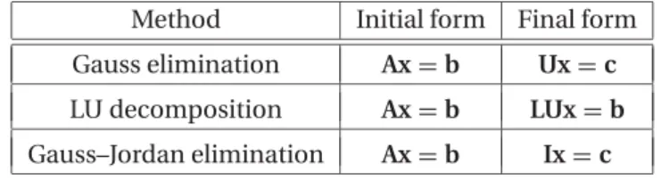
Table 2.1 lists three popular direct methods, each of which uses elementary operations to produce its own ﬁnal form of easy-to-solve equations.

Method Initial form Final form

Gauss elimination Ax=b Ux=c

LU decomposition Ax=b LUx=b

Gauss–Jordan elimination Ax=b Ix=c

Table 2.1

In the above tableUrepresents an upper triangular matrix,Lis a lower triangular

matrix andI denotes the identity matrix. A square matrix is calledtriangular if it

contains only zero elements on one side of the leading diagonal. Thus a 3×3 upper

triangular matrix has the form

U=   

U11 U12 U13

0 U22 U23

0 0 U33

(41)

and a 3×3 lower triangular matrix appears as

L=   

L11 0 0

L21 L22 0

L31 L32 L33

  

Triangular matrices play an important role in linear algebra, since they simplify

many computations. For example, consider the equationsLx=c, or

L11x1=c1

L21x1+L22x2=c2

L31x1+L32x2+L33x3=c3

.. .

If we solve the equations forward, starting with the ﬁrst equation, the computations are very easy, since each equation contains only one unknown at a time. The solution would thus proceed as follows:

x1 =c1/L11

x2 =(c2−L21x1)/L22

x3 =(c3−L31x1−L32x2)/L33

.. .

This procedure is known asforward substitution. In a similar way,Ux=c,encountered

in Gauss elimination, can easily be solved byback substitution, which starts with the

last equation and proceeds backward through the equations.

The equationsLUx=b, which are associated with LU decomposition, can also

be solved quickly if we replace them with two sets of equivalent equations:Ly=b

andUx=y. NowLy=bcan be solved foryby forward substitution, followed by the

solution ofUx=yby means of back substitution.

The equations Ix=c, which are produced by Gauss–Jordan elimination, are

equivalent tox=c(recall the identityIx=x), so thatcis already the solution.

EXAMPLE 2.1

Determine whether the following matrix is singular:

A=   

2.1 −0.6 1.1

3.2 4.7 −0.8

3.1 −6.5 4.1

(42)

Solution Laplace’s development of the determinant (see Appendix A2) about the ﬁrst

row ofAyields

|A| =2.1

4.7 −0.8 −6.5 4.1

−(−0.6)

3.2 −0.8

3.1 4.1

+1.1

3.2 4.7

3.1 −6.5 =2.1(14.07)+0.6(15.60)+1.1(−35.37)=0

Since the determinant is zero, the matrix is singular. It can be veriﬁed that the

singu-larity is due to the following row dependency: (row 3)=(3×row 1)−(row 2).

EXAMPLE 2.2

Solve the equationsAx=b, where

A=   

8 −6 2

−4 11 −7

4 −7 6

 

 b=

   28 −40 33   

knowing that the LU decomposition of the coefﬁcient matrix is (you should verify this)

A=LU=   

2 0 0

−1 2 0

1 −1 1

     

4 −3 1

0 4 −3

0 0 2

  

Solution We ﬁrst solve the equationsLy=bby forward substitution:

2y1=28 y1=28/2=14

−y1+2y2= −40 y2=(−40+y1)/2=(−40+14)/2= −13

y1−y2+y3=33 y3=33−y1+y2=33−14−13=6

The solutionxis then obtained fromUx=yby back substitution:

2x3=y3 x3=y3/2=6/2=3

4x2−3x3=y2 x2=(y2+3x3)/4=[−13+3(3)]/4= −1

4x1−3x2+x3=y1 x1=(y1+3x2−x3)/4=[14+3(−1)−3]/4=2

Hence the solution isx=

2 −1 3

T

2.2

Gauss Elimination Method

Introduction

(43)

formUx=c. The equations are then solved by back substitution. In order to illustrate the procedure, let us solve the equations

4x1−2x2+x3 =11 (a)

−2x1+4x2−2x3 = −16 (b)

x1−2x2+4x3 =17 (c)

Elimination phase The elimination phase utilizes only one of the elementary

op-erations listed in Table 2.1—multiplying one equation (say, equation j) by a constant

λand subtracting it from another equation (equationi). The symbolic representation

of this operation is

Eq. (i)←Eq. (i)−λ× Eq. (j) (2.6)

The equation being subtracted, namely Eq. (j), is called thepivot equation.

We start the elimination by taking Eq. (a) to be the pivot equation and choosing

the multipliersλso as to eliminatex1from Eqs. (b) and (c):

Eq. (b)←Eq. (b)−(−0.5)×Eq. (a)

Eq. (c)←Eq. (c)−0.25×Eq. (a)

After this transformation, the equations become

4x1−2x2+x3=11 (a)

3x2−1.5x3= −10.5 (b)

−1.5x2+3.75x3=14.25 (c)

This completes the ﬁrst pass. Now we pick (b) as the pivot equation and eliminatex2

from (c):

Eq. (c)←Eq. (c)−(−0.5)×Eq.(b)

which yields the equations

4x1−2x2+x3 =11 (a)

3x2−1.5x3 = −10.5 (b)

3x3 =9 (c)

The elimination phase is now complete. The original equations have been replaced by equivalent equations that can be easily solved by back substitution.

(44)

would be written as

  

4 −2 1 11

−2 4 −2 −16

1 −2 4 17

  

and the equivalent equations produced by the ﬁrst and the second passes of Gauss elimination would appear as

  

4 −2 1 11.00

0 3 −1.5 −10.50

0 −1.5 3.75 14.25

  

  

4 −2 1 11.0

0 3 −1.5 −10.5

0 0 3 9.0

  

It is important to note that the elementary row operation in Eq. (2.6) leaves the terminant of the coefﬁcient matrix unchanged. This is rather fortunate, since the de-terminant of a triangular matrix is very easy to compute—it is the product of the diagonal elements. In other words,

|A| = |U| =U11×U22× · · · ×Unn (2.7)

Back substitution phase The unknowns can now be computed by back substitu-tion in the manner described in the previous article. Solving Eqs. (c), (b) and (a) in that order, we get

x3=9/3=3

x2=(−10.5+1.5x3)/3=[−10.5+1.5(3)]/3= −2

x1=(11+2x2−x3)/4=[11+2(−2)−3]/4=1

Algorithm for Gauss Elimination Method

Elimination phase

Let us look at the equations at some instant during the elimination phase. Assume that

the ﬁrstkrows ofAhave already been transformed to upper triangular form. Therefore,

the current pivot equation is thekth equation, and all the equations below it are still to

be transformed. This situation is depicted by the augmented coefﬁcient matrix shown

below. Note that the components ofAare not the coefﬁcients of the original equations

(45)

The same applies to the components of the constant vectorb.                    

A11 A12 A13 · · · A1k · · · A1j · · · A1n b1 0 A22 A23 · · · A2k · · · A2j · · · A2n b2 0 0 A33 · · · A3k · · · A3j · · · A3n b3

..

. ... ... ... ... ... ...

0 0 0 · · · Akk · · · Akj · · · Akn bk ..

. ... ... ... ... ... ...

0 0 0 · · · Aik · · · Ai j · · · Ain bi ..

. ... ... ... ... ... ...

0 0 0 · · · Ank · · · Anj · · · Ann bn                    

← pivot row

← row being

transformed

Let theith row be a typical row below the pivot equation that is to be transformed,

meaning that the elementAikis to be eliminated. We can achieve this by multiplying

the pivot row byλ=Aik/Akkand subtracting it from theith row. The corresponding

changes in theith row are

Ai j ← Ai j−λAkj, j=k,k+1, . . . ,n (2.8a)

bi ←bi−λbk (2.8b)

To transform the entire coefﬁcient matrix to upper triangular form,kandiin Eqs. (2.8)

must have the rangesk=1,2, . . . ,n−1 (chooses the pivot row),i=k+1,k+2. . . ,n

(chooses the row to be transformed). The algorithm for the elimination phase now almost writes itself:

if a[i,k] != 0.0: lam = a[i,k]/a[k,k]

a[i,k+1:n] = a[i,k+1:n] - lam*a[k,k+1:n]

b[i] = b[i] - lam*b[k]

In order to avoid unnecessary operations, the above algorithm departs slightly from Eqs. (2.8) in the following ways:

r _If_A_ik_{happens to be zero, the transformation of row}_i_{is skipped.}

r _{The index} _j _{in Eq. (2.8a) starts with}_k₊_{1 rather than}_k_{. Therefore,} _A_ik _{is not}

(46)

Back Substitution Phase

After Gauss elimination the augmented coefﬁcient matrix has the form

A b

=

       

A11 A12 A13 · · · A1n b1 0 A22 A23 · · · A2n b2 0 0 A33 · · · A3n b3 ..

. ... ... ... ...

0 0 0 · · · Ann bn        

The last equation,Annxn=bn, is solved ﬁrst, yielding

xn=bn/Ann (2.9)

Consider now the stage of back substitution wherexn,xn−1, . . . ,xk+1have been

already been computed (in that order), and we are about to determinexkfrom thekth

equation

Akkxk+Ak,k+1xk+1+ · · · +Aknxn=bk

The solution is

xk=

bk− n

j=k+1 Akjxj

1

Akk

, k=n−1,n−2, . . . ,1 (2.10)

The corresponding algorithm for back substitution is:

x[k]=(b[k] - dot(a[k,k+1:n],x[k+1:n]))/a[k,k]

gaussElimin

The function gaussElimin combines the elimination and the back substitution

phases. During back substitutionbis overwritten by the solution vectorx, so that

bcontains the solution upon exit.

## module gaussElimin ’’’ x = gaussElimin(a,b).

Solves [a]{b} = {x} by Gauss elimination.

’’’

from numarray import dot

def gaussElimin(a,b): n = len(b)

(47)

if a[i,k] != 0.0:

lam = a [i,k]/a[k,k]

a[i,k+1:n] = a[i,k+1:n] - lam*a[k,k+1:n] b[i] = b[i] - lam*b[k]

# Back substitution

b[k] = (b[k] - dot(a[k,k+1:n],b[k+1:n]))/a[k,k] return b

Multiple Sets of Equations

As mentioned before, it is frequently necessary to solve the equationsAx=bfor several

constant vectors. Let there bemsuch constant vectors, denoted byb1,b2, . . . ,bmand

let the corresponding solution vectors bex1,x2, . . . ,xm. We denote multiple sets of

equations byAX=B, where

X=

x1 x2 · · · xm

B=

b1 b2 · · · bm

aren×mmatrices whose columns consist of solution vectors and constant vectors,

respectively.

An economical way to handle such equations during the elimination phase is

to include allmconstant vectors in the augmented coefﬁcient matrix, so that they

are transformed simultaneously with the coefﬁcient matrix. The solutions are then obtained by back substitution in the usual manner, one vector at a time. It would

be quite easy to make the corresponding changes ingaussElimin. However, the LU

decomposition method, described in the next article, is more versatile in handling multiple constant vectors.

EXAMPLE 2.3

Use Gauss elimination to solve the equationsAX=B, where

A=   

6 −4 1

−4 6 −4

1 −4 6

 

 B=

  

−14 22

36 −18

6 7

  

Solution The augmented coefﬁcient matrix is 

 

6 −4 1 −14 22

−4 6 −4 36 −18

1 −4 6 6 7

(48)

The elimination phase consists of the following two passes:

row 2←row 2+(2/3)×row 1

row 3←row 3−(1/6)×row 1

  

6 −4 1 −14 22

0 10/3 −10/3 80/3 −10/3

0 −10/3 35/6 25/3 10/3

  

and

row 3←row 3+row 2

  

6 −4 1 −14 22

0 10/3 −10/3 80/3 −10/3

0 0 5/2 35 0

  

In the solution phase, we ﬁrst computex1by back substitution:

X31=

35

5/2=14

X21= 80/3+(10/3)X31

10/3 =

80/3+(10/3)14

10/3 =22

X11= −14+4X21−X31

6 =

−14+4(22)−14

6 =10

Thus the ﬁrst solution vector is

x1=

X11 X21 X31

T

=10 22 14 T

The second solution vector is computed next, also using back substitution:

X32=0

X22= −10/3+(10/3)X32

10/3 =

−10/3+0

10/3 = −1

X12= 22+4X22−X32

6 =

22+4(−1)−0

6 =3

Therefore,

x2=

X12 X22 X32

T

(49)

EXAMPLE 2.4

Ann×nVandermode matrixAis deﬁned by

Ai j =vni−j, i=1,2, . . . ,n, j=1,2, . . . ,n

wherevis a vector. Use the functiongaussEliminto compute the solution ofAx=b,

whereAis the 6×6 Vandermode matrix generated from the vector

v=1.0 1.2 1.4 1.6 1.8 2.0 T

and

b=

0 1 0 1 0 1

T

Also evaluate the accuracy of the solution (Vandermode matrices tend to be ill-conditioned).

Solution

#!/usr/bin/python ## example2_4

from numarray import zeros,Float64,array,product, \ diagonal,matrixmultiply

from gaussElimin import *

def vandermode(v): n = len(v)

a = zeros((n,n),type=Float64) for j in range(n):

a[:,j] = v**(n-j-1)

return a

v = array([1.0, 1.2, 1.4, 1.6, 1.8, 2.0]) b = array([0.0, 1.0, 0.0, 1.0, 0.0, 1.0]) a = vandermode(v)

aOrig = a.copy() # Save original matrix

bOrig = b.copy() # and the constant vector x = gaussElimin(a,b)

det = product(diagonal(a)) print ’x =\n’,x

(50)

print ’\nCheck result: [a]{x} - b =\n’, \ matrixmultiply(aOrig,x) - bOrig raw_input(’’\nPress return to exit’’)

The program produced the following results:

x =

[ 416.66666667 -3125.00000004 9250.00000012 -13500.00000017 9709.33333345 -2751.00000003]

det = -1.13246207999e-006

Check result: [a]{x} - b =

[-4.54747351e-13 4.54747351e-13 -1.36424205e-12 4.54747351e-13 -3.41060513e-11 9.54969437e-12]

As the determinant is quite small relative to the elements ofA(you may want to

printAto verify this), we expect detectable roundoff error. Inspection ofxleads us to

suspect that the exact solution is

x=1250/3 −3125 9250 −13500 29128/3 −2751

T

in which case the numerical solution would be accurate to about 10 decimal places.

Another way to gauge the accuracy of the solution is to computeAx−b(the result

should be0). The printout indicates that the solution is indeed accurate to at least

10 decimal p