Linear Program Construction Using Metamodeling

(1)

Abstract

PARKS, JUDITH-MARIE TYLER. Linear Program Construction Using Metamodeling. (Under the direction of Thom J. Hodgson.)

One of the most significant trends in data warehousing today is the integration of Metadata

into data warehousing tools. A data warehouse is an area which exists on computer systems

that is used for holding all of the data that an organization might possess. Metadata is ″data about data,″ a dictionary and summary of data, that is held in a system catalog that is contained in a data warehouse. The purpose of this dissertation is four-fold: to show that by

examining a database’s system catalog, information can be extracted from it that can be used

to develop a structure for building operations research applications. To show that a

database’s system catalog can be modified to hold the structure and the definition of a linear

programming model. To show that a data table containing the linear programming model

constraints can be automatically constructed based on the contents of the modified system

catalog. And finally, to show that the modified system catalog can be used to guide a user in

developing objective functions based on a given set of model constraints. Thus, the main

contribution of the work is that it furthers the hybrid area of information

technology/mathematical programming by exploiting metadata, as opposed to raw data, that

(2)

LINEAR PROGRAM CONSTRUCTION USING METAMODELING

By

JUDITH-MARIE TYLER PARKS

A thesis submitted to the Graduate Faculty of North Carolina State University

in partial fulfillment of the requirements for the Degree of

Doctor of Philosophy

INDUSTRIAL ENGINEERING

Raleigh 2002

APPROVED BY:

________________________________ _________________________________

________________________________ _________________________________

________________________________

(3)

ii

Biography

Judith-Marie T. Parks was born on June 16, 1972 in Chicago, Illinois. She attended

Rensselaer Polytechnic Institute in Troy, New York from 1990 – 1995 and graduated with a

Bachelor of Science degree in Decision Sciences and Engineering Systems. In August 1995,

Judith-Marie enrolled in graduate school at North Carolina State University where she earned

a Masters degree in Industrial Engineering in December 1997 and a Ph. D. in Industrial

(4)

iii

Acknowledgements

I would like to thank my family for being a constant source of support, in particular my

mother, Irma Parks. I would also like to thank “the best committee in the world” – Dr. Thom

Hodgson, Dr. Robert Young, Dr. Marc Cohen, Dr. Russell King, and Dr. Michael Kay - for

your many words of encouragement and support during the many tough times. In addition, I

would like to acknowledge the following people for their friendship, kindness, support,

patience, and understanding: Jennifer, Shona, Shree, Jodie, Andres, Ali, Don, and Chuck for

(5)

iv

Contents

List of Tables ... vi

List of Figures ... viii

1. Introduction... 1

2. Related Work ... 4

2.1 Model Formulation and Knowledge Acquisition ... 4

2.2 Model Management ... 6

3. Research Context ... 8

4. Objectives of This Dissertation... 10

5. An Example of a System Catalog ... 13

5.1 Illustration of the System Catalog... 14

5.2 Highlighting Information in a System Catalog... 25

5.3 Summary... 30

6. Analysis and Exploitation of the System Catalog... 31

6.1 The General Data Dependency Structure ... 31

6.2 The Linear Programming Model Dependency Structure... 34

6.3 The Correlation Between the Data Dependency Structure and the Linear Programming Model Dependency Structure ... 37

6.4 The Auxiliary Catalog... 39

6.5 Summary... 60

7. Analysis and Exploitation of a Large Database... 61

7.1 Issues Surrounding Large Databases ... 61

(6)

v

8. Summary ... 73

8.1 Features of the Methodology ... 73

8.2 Relation to Other Work... 74

8.3 Future Work ... 74

REFERENCES ... 75

(7)

vi

List of Tables

Table 5.1: Table describing the relationships among the tables in the Advertising database. 27

Table 6.1: Example model data in database table Cost_Data... 50

Table 6.2: Example model data in database table Demographics. ... 50

Table 6.3: LP Model Extraction Table. ... 50

Table 6.4: LP Model Extraction Table after Step 1. ... 52

Table 7.1: Subset of records from the Objective Function auxiliary system catalog table. ... 65

Table 7.2: Subset of records from the Constraint auxiliary system catalog table... 68

Table 7.3: Subset of Plants data... 69

Table 7.4: Subset of Fcost data ... 70

Table 7.5: Subset of Invcap data... 70

Table 7.6: Subset of Demand data ... 70

Table 7.7: LP Model Extraction Table. ... 71

Table A.1: Transportation database system catalog – Database Table Component. ... 77

Table A.2: Transportation database system catalog – Table Table Component... 78

(8)

vii Table A.3: Transportation database system catalog – Column Table Component... 82

Table A.3 (continued): Transportation database system catalog – Column Table Component.

... 85

Table A.4: Transportation database system catalog – Primary Key Table Component. ... 86

(9)

viii

List of Figures

Figure 5.1: Example system catalog metadatabase... 15

Figure 5.2: Changes to the system catalog tables after performing Action 1. ... 20

Figure 5.3 (a): Changes to the system catalog tables after performing Action 2. ... 21

Figure 5.3 (b): Additional changes to the system catalog tables after performing Action 2.1 ... 22

Figure 5.4 (a): Changes to the system catalog tables after performing Action 3. ... 24

Figure 5.4 (b): Changes to the system catalog tables after performing Action 3... 25

Figure 5.5: Entity-Relationship model of the Cost_Data and Demographics data tables. ... 29

Figure 6.1: General two-table example of a data dependency structure... 33

Figure 6.2: A general data dependency structure as it relates to our previous example... 33

Figure 6.3: The dependency structure of a linear programming model... 36

Figure 6.4: The correlation between the data dependency structure and the dependency structure of a linear programming model... 39

Figure 6.5: The auxiliary catalog including the new OBJECTIVE FUNCTION, CONSTRAINT, and MODEL MATCH components. ... 41

Figure 6.6: Example linear programming model formulation... 51

Figure 6.7: Linear programming model solution... 60

Figure 7.1: Example linear programming model formulation... 71

Figure 7.2: Linear programming model solution... 72

Figure A.1: Definition of the auxiliary component tables of the auxiliary system catalog. ... 88

(10)

1

Chapter 1

1. Introduction

A significant trend in the development of data warehousing is the integration of metadata into

warehousing tools (Ref. Poe et al., 1998). Metadata is defined as, ″data about data″, a

dictionary and summary of data, according Hsu (1996) and V. Poe et al. (1998). For example,

assume momentarily that data can be interpreted as a program for improving business

functions, then metadata is information about that program. Metadata is an account of what

the program does, and contains specifics on how it improves business functions. Contained

within the metadata are rules about, and relationships among, lower level data.

Metadata can be used as a tool used for analysis as well as for knowledge management.

Many companies find that after investing heavily in distributed computer networks in order

to give more people better access to business knowledge, the company’s goals are not

achieved because it is still too difficult to locate or develop the desired information. In

addition, company mergers can and have wreaked havoc on organizations' information

systems. Metadata is a consolidated representation of data and as such, it can be derived from

multiple data and knowledge systems. Consequently, a metamodel can handle multiple data

and knowledge systems, making the methodology useful across multiple data platforms.

Metadata provides organizations with a way to understand, organize, and exploit information

(11)

2 metadata to construct mathematical constraints is the purpose of the work proposed here. To

do this, we focus on one form of metadata associated with relational database systems.

In an attempt to develop enterprise models for analysis and optimization, information

technology consultants can spend months at client sites configuring and reconfiguring data

models (e.g., entity relationship models) in order to make sure the model contains business

rules that are valid for the client. These entity relationship models are also represented in the

database system catalog where the database tables are implemented. Thus, the database

system catalog holds valid business rules for a corporation. The information that is held in

the system catalog is referred to as metadata. Therefore, if the valid business rules needed for other types of modeling could be automatically inferred from the metadata, significant

timesavings in the development of those models could be achieved.

By using the information held in the system catalog to understand and analyze relationships

among data, a great amount of knowledge about an organization can be acquired.

Furthermore, analyzing and uncovering specific data relationships can contribute to the

information asset base of an organization either by helping it to operate more efficiently or

by discovering new information on which the organization can capitalize. Given sufficient

metadata, use of this higher level data can make the task of data relationship analysis more

time efficient than developing each model from the beginning using raw data.

Areas that can benefit from this work cover a wide range. They comprise areas that depend

(12)

3 such as bioinformatics where a potential use is reducing redundancy in experimentation by

electronically discovering genetic relationships that, at least mathematically, appear to yield

optimal results. Similarly, this concept has potential uses in the chemical and pharmaceutical

industries where discovering certain relationships, combined with optimization modeling can

lead to the discovery of new compounds or materials. The military may find it useful for

tasks such as targeting battlefields or strategic planning. The area of focus of this work is

enterprise strategic planning. Specifically, we will use metadata to understand and analyze

the relationships that exist among raw data, then use that information to construct linear

programming constraints related to optimal marketing strategies.

The remainder of this document is organized as follows: The Related Work section reviews work done in the area. The Research Context section provides background and sets the stage for our work. The Research Objectives section describes the objectives that need to be fulfilled in order to achieve our goal. The remaining sections provide a description of how

(13)

4

Chapter 2

2. Related Work

Research related to the area of metamodeling has been conducted in two main areas: model

formulation systems and model management systems. Each of these areas is described in

terms of the scope that they cover, the general backgrounds that support them, and their

historical contributions. We then highlight corresponding research issues, discuss the focus

of the research, and establish how the work contributes to the resolution of some of these

issues.

2.1 Model Formulation and Knowledge Acquisition

Model formulation is concerned with acquiring knowledge, developing computer systems

that use this knowledge as high-level input about a situation, and then formulating a

mathematical model accordingly. The input to the model is a representation of the physical

system rather than a math model itself, as is generally the case with modeling languages (e.g.

Lindo, GAMS, etc.). Research in this area has benefited primarily from the operations

research, statistics, and artificial intelligence disciplines. Literature discussing work of this

nature can commonly be found in operations research, management science, decision

(14)

5 In general, the research focuses on using techniques such as constraint satisfaction

(Raghunathan 1992) and structured modeling (Raghunathan 1996) to formulate models.

More recently, data visualization techniques such as metagraphs have been used for model

formulation (Basu and Blanning 1997, Dombrovskaia, Rodriguez, and Nussbaum 1998).

Raghunathan (1992) develops logical constraints based on a specific domain situation, as a

way to represent that situation in logical form. He then uses constraint satisfaction theory to

convert the logical constraints into the linear constraints that comprise a mathematical model.

In later work, Raghunathan (1996) uses the structured modeling framework together with

SML - Structured Modeling Language (Geoffrion 1987) - to model and design a decision

support system. Though these are valuable contributions, they lack robustness in that they are

limited to specific domains (e.g., the production domain) and certain classes of problems.

Research in this area has evolved to become more comprehensive in scope. Basu and

Blanning (1997) use metagraphs, a graph-theoretic construct, to visualize a knowledge base

structure whose information is then used as input to a model. The knowledge base consists of

data, decision models, and expert knowledge in the form of rules. The metagraphs are then

used to analyze the various components in order to make useful inferences during problem

solving. Similarly, Dombrovskaia, et. al (1998) illustrate a knowledge-based modeling

methodology that allows LP problems to be specified in a graphic and declarative way using

graphic objects and their semantics. These two approaches are more progressive than the

former approaches in that they show increased focus on data issues and relationships among

(15)

6 sophisticated approach to solving some of the data (knowledge acquisition) issues that are

present in model formulation.

2.2 Model Management

Model management research, in the context of decision support systems (DSS), deals with

allowing flexible accessing, updating, and altering of standard models (e.g., Linear

Programming) for the purpose of more efficient model use. Research in this area has

benefited from a hybrid of different fundamental technologies such as database management

systems, artificial intelligence, and the World Wide Web. Historically, numerous articles on

model management systems have appeared in the DSS literature. However, it is becoming

increasingly common for this type of research to be discussed in computer science journals as

well.

Model management systems have focused on managing the math modeling process

(Raghunathan 1992, Muhanna and Pick 1994) or the models themselves (Kwon and Park

1996). Recently, research has begun to look at the role that raw data play in model

management (Dolk 1999). For example, Raghunathan (1992) developed a modeling system

based on a model of an expert formulation process. A model of the knowledge about the

production domain, a metamodel, was the primary knowledge source that was used in

identifying constraints and dependency relations among entities in the production system. A

model revision component was then developed which uses a dependency network, generated

by the metamodel and a truth maintenance system, to reformulate and represent different

(16)

7 and Pick (1994) involves a framework that suggests a graph-oriented, non-procedural, and

hierarchical (i.e., top-down) approach for model synthesis. However, like Raghunathan

(1992), underlying the framework is a set of metamodeling concepts that capture the

semantics of the modeling process, as opposed to the semantics of the input data. Kwon and

Park (1996) focus on the concept of model re-use using a framework that facilitates

interpretation of models, extraction of model constructs, and model construction. They

collect modeling knowledge that is explicitly or implicitly associated with existing models.

The aforementioned work is among the many approaches that focus on the modeling process

as a foundation for model management. However, recent approaches focus more on the data

issues that surround the mathematical modeling. Dolk (1999) uses an approach that involves

the relationships between modeling and data warehouses. He develops decision metrics as a

foundation for what information a decision-oriented database should contain. Decision

metrics provide readily understandable problem identification cues that can then be tied to

decision models for subsequent problem diagnosis and sensitivity analysis. This is an

appealing approach, as it tackles an important area in optimization; good input data. This

(17)

8

Chapter 3

3. Research Context

Every relational database management system (RDBMS) must provide a catalog or

dictionary function to support all of the databases and tables that exist within the system. The

system catalog and the metadata information contained within it are both instantiated upon

initial creation of a database. The system catalog contains detailed information regarding the

various database objects that are of interest to the system itself. It holds information such as

indices, user security constraints, and integrity constraints. It also holds information

describing relationships and object existence conditions within the database tables, between

the tables, and between the databases. This system catalog information for a relational database is also held in a relational database. Because of this, as long as administrative privileges have been granted, a user can execute queries on the system catalog in the same

way that they execute queries on any relational database. This provides a user with access to

the system catalog and its metadata.

Date's (2000) description of a system catalog is a generic representation of the contents of

system catalogs in general. SQL Server, DB2, Sybase, and Oracle are the four major

commercially available relational database management systems, together comprising

roughly 90% of the DBMS market. Their system catalogs contain similar types of

information. For example, SQL Server contains a centralized system catalog that holds the

(18)

9 items such as database objects, constraints, user identities, and user permissions. In addition,

the centralized catalog contains some information about individual databases such as

database names, primary file locations, database configuration values, and login accounts.

Similarly, the knowledge base of every data object known to DB2 is stored in the DB2

system catalog. The contents of the catalog consist of entries such as system constraints,

update privileges held by a user, information about links between the catalog tables, stored

procedures, statistics on frequently occurring values in a column, and referential integrity for

every relationship defined in DB2. The Sybaseand Oracle system catalogs both function

in virtually the same way as the SQL Serverand DB2 catalogs, as they are similar in both

structure and content. In both cases the catalogs hold tables that contain constraints, indexes,

user privileges, database link information, and stored procedures. Another DBMS, SAS has

a relational database system catalog that is similar in structure and content as the four major

systems. The SAS system is the platform upon which a larger part of our work is built,

simply because that is the system that was available for us to use. That said, the previous

descriptions of the four major DBMS's are consistent with the description that Date (2000)

provides. As such, Date's (2000) description is a sufficient reference for future general

(19)

10

Chapter 4

4. Objectives of This Dissertation

There are four main objectives of this dissertation. They are as follows:

1. To show that by examining a relational database’s system catalog, information can be

extracted from it that can be used to develop a structure for building linear programs.

A system catalog is an administrative relational database that holds the identity and

structure of lower-level, relational databases. The characteristics of the system catalog are

such that it contains, among other things, information on the relationships and

dependencies within an individual database and between databases. It is because of the

linear nature of the relational database that it can be exploited and mapped into the

structure of linear programming models.

2. To show that a system catalog can be modified to hold the structure and the definition of

a linear programming model, and that the modifications are consistent with the intent and

structure of the original system catalog.

A model structure represents the basic form of a linear program, such as the decision

variables. A model definition represents that which explicitly identifies appropriate data

(20)

11

consistent with the original catalog refer to the part of the modified system catalog structure that is derived from the original system catalog structure. An example would be

a keyword structure that might describe the type of model being constructed. The remaining modified system catalog modifications result from translating the original

catalog entries into the structure and definition of a linear programming model.

3. To show that a data table containing the linear programming model constraints can

automatically be constructed based on the contents of the modified system catalog.

The basic model structure (i.e., formulation) can be extracted from the structure of the

modified system catalog as a foundation for the linear programming model. The model

coefficients can be extracted by using the modified system catalog model definitions as a

guide for identifying appropriate data to extract from individual database tables.

4. Finally, to show that the modified system catalog can be employed to guide a user in

developing objective functions based on a given set of model constraints.

The set of objective functions that can be combined with model constraints is based either

on an entire set of available constraints or a subset of constraints that are extracted from

the modified system catalog. Available constraints refers to the set of constraints that can be formulated based on both the contents of the individual database tables, and the level

(21)

12 Recall from the second objective that this knowledge is obtained by examining the

(22)

13

Chapter 5

5. An Example of a System Catalog

Now that we have defined a system catalog and established the purpose for its existence, we

describe an example of a catalog. We begin with an introduction of the example system

catalog that we use in the illustration. We offer brief descriptions of each catalog table as

well as how the tables relate to each other. We then take the reader, step by step, through an

illustration of how each table is populated. Finally, we show that queries can be executed on

the system catalog tables for the purpose of highlighting information that defines the

relationships among all of the tables in the database. However, prior to these tasks, we make

a clarification regarding the exhaustiveness of the list of tables in our example catalog.

Figure 5.1 lists all of the tables that exist in our example system catalog. This list is

non-exhaustive, as it represents only the portion of a system catalog that relates to inter- and

intra-relationships among the database tables. According to Date (1997), this portion of the system

catalog falls under the Base Table Definitions component of the entire system catalog. The other components of the system catalog include the following: Domain, View, Grant,

Constraint, Character Set, Collation, and Translation definitions. The scope of the work is limited to the Base Table Definitions category. As such, we do not elaborate on the other categories of definitions here. However, the interested reader may refer to Date (1997) for an

(23)

14

5.1 Illustration of the System Catalog

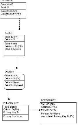
The example system catalog metadatabase, shown in Figure 5.1, consists of the following

tables: The Database table, the Table table, the Column table, the Primary Key table, and

the Foreign Key table. In the figure, these tables are represented by boxes, above which the

name of the table is shown. Within each box is a list of names which are the names of the

columns that are in the table. In each box the names are divided by a line. The purpose of that

line is to identify the names of the columns that comprise the primary key (PK) in each table

from the names of the columns that are non-keys in each table. The names of the columns

that comprise the primary key are above the line, while the names of the columns that are

non-keys are below the line. Further details on this topic can be found in the aside entitled “A

Note on Keys and Table Dependency”. Finally, a line that exists between boxes indicates that

there is a relationship between the tables that those boxes represent. For example, the first

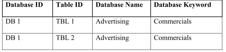
box in Figure 5.1 represents the Database table. The database table contains the columns

Database ID, Table ID, Database Name, and Database Keyword. The Database ID and Table

ID columns are above the line that is drawn inside of the box, indicating that they are the

primary keys in the Database table while the Database Name and the Database Keyword

columns are below the line indicating that they are non-keys. A line exists that originates at

the box representing the Database table and terminates at the box representing the Table

table, indicating that a relationship exists between the two tables. A detailed description of

(24)

15 (Note: The Associated Primary Key is the Primary Key ID inherited from the Primary Key table and renamed)

(25)

16 The system catalog, which is based on the SQL standard (Ref. Date 1997), consists of the

following tables:

• The DATABASEtable:

This table contains a unique identifier for each database held in the database

management system (Database ID), and a unique identifier for each table in each database (Table ID). Taken together, they uniquely associate a Database Name and

Database Keyword with these ID values. Therefore, when a database is created by a user, it is given a Database Name and a Database Keyword describing the purpose for database. All of this information is provided by the user. Subsequently, the

database management system generates a unique Database ID for each database that has been added, a unique Table ID for each table in each database, and associates them, through the DATABASE table, with a Database Nameand a Database Keyword.

• The TABLE table:

This table contains a unique identifier for each table held in a database (Table ID), and a unique identifier for each column in each table (Column ID). Taken together, they uniquely associate a Table Name, Database ID, and a Table Keyword with these ID values. When a table is created by a user, it must be created with at least one

column. The user then provides a Table Name, and a Table Keyword describing the purpose for the existence of the table. Subsequently, the database management system

(26)

17 added. It then generates a unique Column ID in the TABLE table for each column in the table. It migrates the unique Database ID and Table ID from the DATABASE

table. Finally, the database management system associates the Table ID and Column ID, through the TABLE table, to the Table Name, Database ID, and Table Keyword.

• The COLUMN table:

This table contains a unique identifier for each table held in a database (Table ID), and a unique identifier for each column in each table (Column ID). Taken together, they uniquely associate a Column Name and Column Keyword with these ID values. When a column is created by a user, the user provides it with a Column Nameand

Column Keyword describing the purpose for the existence of the column. Subsequently, as columns are added to tables, the database management system

generates a unique Column IDin the TABLEtable for each column that is added. It then migrates the unique Column ID(s) and Table ID from the TABLE table. The database management system then associates the Table ID and Column ID, through the COLUMN table, to the Column Name and Column Keyword.

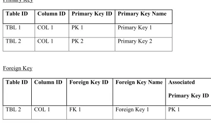
• The PRIMARY KEY table:

(27)

18 The primary key is a column or set of columns that comprise a set of values uniquely

identifying each row in a table. The user then provides the primary key with a

Primary Key Name. Subsequently, the system generates a Primary Key ID in the

PRIMARY KEY table, migrates the Table ID and the Column ID from the

COLUMN table, and associates these three fields with a Primary Key Name.

• The FOREIGN KEY table:

This table contains a unique identifier for each table held in a database (Table ID), a unique identifier for each column in each table (Column ID), and a unique identifier for each foreign key held in a table (Foreign Key ID). Taken together, they uniquely associate a Foreign Key Name, and the associatedPrimary Key ID (Associated Primary Key ID) with these ID values. When a table is fully defined, and if any part of it is derived from another table, it is given a foreign key that is provided either by

the user or the system. Similar to a primary key, a foreign key is defined as a column

or set of columns that comprise a set of values that uniquely identifies a row in a

table. The difference between the two is that a foreign key exists if the user has

created a table from a previously established table using the previously established

table’s primary key columns as some of its columns. Upon creating the foreign key,

(28)

19

ID from the PRIMARY KEY table, and associates these four fields with a Foreign Key Name.

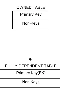
A Note on Keys and Table Dependency: If a table derives any part of its primary key (PK)

from the primary key of another table(s), that table is said to be dependent on the table(s)

from which it derives all or part of its primary key which is indicated by a dotted line relating

the tables. The effect of this is that a data record that exists in a dependent table cannot exist

without first existing in the independent table. If a table derives 100% of its primary key as a

foreign key (FK), then that table is said to be fully dependent on the table from which it

derived its key. In Figure 5.1, this scenario is identified by a solid line connecting the tables.

Conversely, if none of the components of a table’s primary key is derived from another table,

that is no foreign key(s) exist within it, the table is said to be an owned or fully independent

table. An owned or fully independent table is a table that can exist in a database independent

(29)

20 The following is an illustration of how the example system catalog is populated:

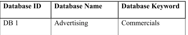
Action 1. We establish the existence of a new database called Advertising. We do this by

logging onto a database management system and opening a new database. This action

prompts the following changes, shown in Figure 5.2, to the tables of the example system

catalog.

Database

Database ID Database Name Database Keyword

DB 1 Advertising Commercials

(30)

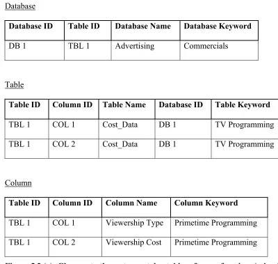
21 Action 2. We establish the existence of a new table called Cost. We do this by executing

the following SQL statement:

CREATE TABLE Cost_Data ([Viewership Type] TEXT (32), [Viewership Cost] TEXT (32), Constraint Names_Pk Primary Key ([Viewership Type]));

This action prompts the following changes, shown in Figures 5.3 (a) and 5.3 (b), to the

tables of the example system catalog.

Database

Database ID Table ID Database Name Database Keyword

DB 1 TBL 1 Advertising Commercials

Table

Table ID Column ID Table Name Database ID Table Keyword

TBL 1 COL 1 Cost_Data DB 1 TV Programming

Column

Table ID Column ID Column Name Column Keyword

TBL 1 COL 1 Viewership Type Primetime Programming

TBL 1 COL 2 Viewership Cost Primetime Programming

(31)

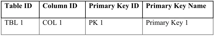
22 In addition, with respect to identifying the primary key this action prompts the following

changes, shown in Figure 5.3 (b), to the tables of the example system catalog.

Primary Key

Table ID Column ID Primary Key ID Primary Key Name

TBL 1 COL 1 PK 1 Primary Key 1

Figure 5.3 (b): Additional changes to the system catalog tables after performing

(32)

23 Action 3. We establish the existence of a second new table called Demographics. We do

this by deriving it from the Cost_Data table executing the following SQL statement:

CREATE TABLE Demographics ([Viewership Type] TEXT (32), [Female Viewership] TEXT (32), [Male Viewership] TEXT (32), [Viewership Requirement] TEXT (32), Constraint Names_Fk Foreign Key ([Viewership Type]) References Cost_Data);

This action prompts the following changes, shown in Figures 5.4 (a) and 5.4 (b), to the

(33)

24 Database

Database ID Table ID Database Name Database Keyword

Table

Table ID Column ID Table Name Database ID Table Keyword

TBL 2 COL 1 Demographics DB 1 Gender

Column

Column ID Table ID Column Name Column Keyword

COL 1 TBL 1 Viewership Type Primetime

COL 2 TBL 1 Viewership Cost Range

COL 1 TBL 2 Viewership Type Primetime

COL 2 TBL 2 Female Viewership Range

COL 3 TBL 2 Male Viewership Range

COL 4 TBL 2 Viewership Requirement Capacity

(34)

25 Primary Key

Table ID Column ID Primary Key ID Primary Key Name

Foreign Key

Table ID Column ID Foreign Key ID Foreign Key Name Associated

Primary Key ID

TBL 2 COL 1 FK 1 Foreign Key 1 PK 1

Figure 5.4 (b): Changes to the system catalog tables after performing Action 3.

5.2 Highlighting Information in a System Catalog

In addition to holding information that describes how data are related to one another, another

functionality of the system catalog is its ability to have queries executed against it in order to

highlight specific information about the data using the conditions set forth in the query.

Recall that this functionality exists because the system catalog is itself, a relational database.

For example, by executing a series of SQL commands on a system catalog, we can generate a

list of all of the columns and tables that exist in a database, the table’s primary key, and the

foreign key(s) that is associated with the table(s). When taken together, this information

describes (in tabular form) how all of the data within a database are related to one another.

Therefore, if one needs to know how the COST_DATA and DEMOGRAPHICS tables from

(35)

26 other, executing a series of SQL commands on the system catalog will highlight such

information. It will list of all of the columns in the two tables, the primary keys

corresponding to each of the tables, and the foreign key for the DEMOGRAPHICS table.

Together, these results define how all of the data in the Advertising database, are related to

one another. The query is shown below:

SELECT

Column.[Column Name], Table.[Table Name], [Primary Key].[Primary Key ID],

[Foreign Key].[Foreign Key ID], [Foreign Key].[Associated Primary Key ID] INTO

[Relationship Table ]

FROM

[Database]

INNER JOIN

((([Table]

LEFT JOIN

[Column] ON (Table.[Column ID] = Column.[Column ID]) AND

(Table.[Table ID] = Column.[Table ID]))

LEFT JOIN

[Primary Key] ON (Column.[Column ID] = [Primary Key].[Column

ID]) AND (Column.[Table ID] = [Primary Key].[Table ID]))

(36)

27 [Foreign Key] ON ([Primary Key].[Column ID] = [Foreign

Key].[Column ID]) AND ([Primary Key].[Table ID] =

[Foreign Key].[Table ID]))

ON

Database.[Table ID] = Table.[Table ID]

WHERE

((([Database].[Database Name])='Advertising') AND (([Database].[Database

Keyword])='Commercial'));

The results of this query are shown in Table 5.1.

Column Name Table Name Primary

Key ID

Foreign

Key ID

Associated

Primary Key

Viewership Type Cost_Data PK 1

Viewership Cost Cost_Data

Viewership Type Demographics PK2 FK 1 PK 1

Female Viewership Demographics

Male Viewership Demographics

Viewership Requirement Demographics

Table 5.1: Table describing the relationships among the tables in the Advertising

(37)

28 Using this information, a graphical representation of the data relationships (i.e., the data

structure) can be constructed. In general, this is done by first identifying, for every table in a

database, the independent table(s) and their corresponding dependent table(s). Based on

information such as that which is found in Table 5.1, an independent table is a table that is

listed in the Table Name column for which there is no associated foreign key. What this implies is that none of the columns comprising the independent table’s primary key is

derived from any other table. Conversely, a dependent table is a table listed in the Table Name column for which there is an associated foreign key. What this implies is that at least one of the columns comprising the dependent table’s primary key is derived from another

table. In addition, all of the columns that make up each table is identified. A line is drawn

between tables indicating that a relationship exists between them. The line originates at the

independent table and terminates at the dependent table. In cases for which there is no

relationship defined, a line does not exist. Such a figure is referred to as an ICAM Definition

Language, or IDEF1X, model and is a widely used entity attribute information modeling tool

(Ref. NIST 93 IDEF1X standard). In our example, the information found in Table 5.1

suggests that a line be drawn originating at the independent table, COST_DATA, and

terminating at the dependent table, DEMOGRAPHICS. Figure 5.5 shows the IDEF1X model

(38)

29

Figure 5.5: Entity-Relationship model of the Cost_Data and Demographics data tables.

As can be seen from the figure, the DEMOGRAPHICS table is created using the primary

key from the COST_DATA table. This makes the Viewership Type column in the

DEMOGRAPHICS table a foreign key whose associated primary key is the Viewership

Type column in the COST_DATA table. The primary key and the foreign key are denoted as

(PK) and (FK), respectively. Thus, the DEMOGRAPHICS table is fully dependent on the

COST_DATA table. As mentioned in the previous section, the owned or fully independent

table(s) in a database can be determined by identifying the table(s) for which the Primary

Key ID column contains a non-null value, while the corresponding Foreign Key ID column

contains a null value. Therefore, according to the information in Table 5.1, the COST_DATA

table is an owned table since it only has a primary key associated with it. The value of this

information will become more apparent in Section 6 where we explore modifying the system

(39)

30

5.3 Summary

After establishing the existence of a system catalog, we illustrated an example of how a

catalog works. In doing so, we showed the structure of our example catalog, provided a brief

description of the tables and columns it contains, and then showed step-by-step how the

system catalog tables are populated. Finally, we showed that by executing a series of SQL

commands on the system catalog, we can extract from the catalog, specific information

which describes the relationships that exists among all of the tables in a database. We further

showed how such information could be translated into an IDEF1X model that is a graphical

(40)

31

Chapter 6

6. Analysis and Exploitation of the System Catalog

In this section we present a picture of how the system catalog can be viewed as a tool for

efficiently defining linear programming models. We elaborate on the dependency structure of

data as determined from the system catalog. We explore the dependency structure of the

elements in a linear programming model. We then show the correlation between the two

structures. Finally, we show that the information about the correlation between the two

structures can be used to represent the fundamental elements of a linear programming model

within a system catalog component, and that this new component can be added to the existing

system catalog in such a way as to directly store all of the fundamental information that is

needed to construct a linear programming model, thereby creating the ability to extract linear

programming models from the system catalog.

6.1 The General Data Dependency Structure

In the previous section we established the fact that information describing the relationships

that exist among data, is held in a system catalog. We further established that fact that this

information can be isolated, extracted from the system catalog, and used to create a graphical

(41)

32 performed in order to show the process by which one can extract from the system catalog the

dependency structure of specific data, presenting it in both tabular and graphical forms.

The data dependency structure identifies, among other things, the owned table(s), fully

dependent table(s), and the level of dependency of all other table(s) within a database. Recall

from the previous section that an owned table is a table that can exist independent of any

other table in a database. It can do this because none of the components of its primary key or

non-key columns are derived from any other tables. Therefore, an owned table’s existence is

not derived from, or a function of, any other table in the database. Similarly, a fully

dependent table is a table whose existence is based entirely on another table or set of tables.

This is so because 100% of its primary key is derived from another table(s) as a foreign key.

As such, its existence is completely a function of at least one other database table. The level

of dependency for all other database tables varies depending on the proportion of the primary

key or the proportion of the total number of columns that are derived from other tables. The

level of dependency can also be dictated by the number of tables that a given table is dependent upon. Analyzing the level of dependency of a given table is an elaborate process

and is outside of the scope of this dissertation. As such, it will not be discussed further here.

Instead, our intention is to simply convey the idea that there is value in using the system

catalog to establish the dependency structure of data. A general, two-table example of a

(42)

33

Figure 6.1: General two-table example of a data dependency structure.

With respect to our previous example, this translates into the same dependency structure that

is shown in Figure 5.6. The details of the translation are shown in the following figure.

Figure 6.2:A general data dependency structure as it relates to our previous example.

Non-Keys Primary Key OWNED TABLE

Non-Keys Primary Key(FK) FULLY DEPENDENT TABLE

Cost

Viewership Type (PK) COST

Female Viewership Male Viewership Viewership Requirement Viewership Type (FK) DEMOGRAPHICS Non-Keys

Primary Key OWNED TABLE

(43)

34 In the next sub-section, we discuss the general dependency structure of a typical linear

programming model.

6.2 The Linear Programming Model Dependency Structure

In this sub-section, we explore the dependency structure of a linear programming model. We

use, as an example, a simple 2-variable, 2-constraint model.

The Linear Programming Model

Minimize z = c1×1 + c2×2 Subject to a11×1 + a12×2 ≥ b1

a21×1 + a22×2 ≤ b2

A number of dependencies and independencies exist in this model. They are as follows:

• The definition of the decision variables in the objective function are independent of the definitions of any other component in the model. That is, their definition is not a function

of, derived from, nor does it depend on any other component in the model. Therefore, the

definition of decision variables in the objective function are fully independent of all other

coefficients and variables in the model. Note that from here on out, when we refer to a

(44)

35 subscript, unless otherwise noted. Since the decision variable has no value before the

model is solved, it is more precise to say that it is the subscript accompanying the

decision variable that is independent. In the interest of clarity, we find it simpler to refer

to the object that the subscript accompanies and identifies with as opposed to the

subscript itself.

• The coefficients in the objective function are defined as a function of their corresponding decision variable. Therefore, the definition of the coefficients in the objective function is

dependent on the decision variables in the objective function.

• The decision variables in the constraints are, in this case, exactly the same as the decision variables in the objective function and as such, their definitions are fully dependent on

the objective function decision variables. In general, variables that are in constraints but

not in the objective function can be defined. These variables would then be indirectly

dependent on the decision variables in the objective function and defined based on

variables that are directly dependent on the decision variables in the objective function. A

constraint variable that does not meet this condition would have no relevance to the

model’s solution whatsoever and would thus be a trivial and unnecessary constraint.

• The coefficients in the constraints are defined as a function of their corresponding decision variable. Therefore, the definition of the coefficients in the constraints is

dependent on the decision variables in the constraints. Note that since it is the case here

that all of the constraint decision variables are fully dependent on the objective function

decision variables, the definition of the constraint coefficients is dependent on the

objective function’s decision variables, as is the case with the objective function

(45)

36

• The definition of the b-vector is a function of the left side of the constraint. That is, the decision variables in the constraints are the primary elements of the model upon which

the information that is used to define the b-vector is based.

In general, the dependency structure of a linear programming model is as follows:

Figure 6.3:The dependency structure of a linear programming model.

In the next sub-section, we discuss the correlation between the dependency structure of a

linear programming model and the dependency structure of data as described by the system

catalog.

A B X (FK) CONSTRAINT C

X

(46)

37

6.3 The Correlation Between the Data Dependency Structure and the Linear

Programming Model Dependency Structure

There is a correlation between the dependency structure of data as described in a system

catalog, and the dependency structure of a linear programming model. The structures

correspond in the following way:

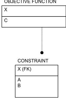
• The properties that define an owned table – as a table that is defined independent of any other table of a group of tables and is also the table from which all other dependent tables

are derived – also define an objective function, as its definition is fully independent of the

remaining components of a linear programming model. Similarly, the properties that

define the primary key in an owned table – as an entity that defines the fundamental

elements of a row in a table as well as helping to define dependent tables – also define the

decision variables in an objective function, as they define the fundamental elements of

the objective function as well as (either directly or indirectly) the constraints in a linear

programming model. Finally, the properties that define a non-key in an owned table – as

an entity whose definition depends only on, and is a function of the primary key in the

owned table – also holds for the coefficients in the objective function, as they are a

function of, and depend only on, the fully independent objective function decision

variables. This is consistent with third normal form in database management systems

(Ref. Date, 2000). Third normal form states that all elements in a row are uniquely

identified by the primary key in a table and nothing else. That is, there is no functional

(47)

38

• The property that defines the fully dependent table – as an entity whose definition is completely derived (either directly or indirectly) from another table – also holds for the

constraints in a linear programming model. Similarly, the property that defines the

primary key in a fully dependent table – as a table that fully derives its fundamental

components (i.e. primary key) from another table’s fundamental components – also holds

for the decision variables in the constraint that are defined by, and derived from, the

decision variables in the objective function. The property that defines the non-keys in a

fully dependent table – as an entity whose definition depends on the primary key in its

own table – also holds for the coefficients and the b-vector in the constraint, as they both

exist as a function of the fully dependent decision variables in the constraint.

(48)

39

Figure 6.4:The correlation between the data dependency structure and the dependency

structure of a linear programming model.

In the Section 6.4, we discuss how these elements are represented in new system catalog

components.

6.4 The Auxiliary Catalog

In this section, we show how the fundamental elements of a linear programming model can

be represented as additional components of a system catalog. We call these new components

auxiliary components. The auxiliary components are included as part of the existing system catalog and are indirectly related to the original system catalog components by way of

functional transformations and information mapping. Information is collected from the

original system catalog, transformed, and mapped into the auxiliary components. The A

B X (FK) CONSTRAINT C

X

OBJECTIVE FUNCTION

Non-Keys Primary Key OWNED TABLE

(49)

40 auxiliary components are held in the system catalog, however, as stand-alone entities

separated from the other catalog components. These auxiliary components store all of the

fundamental information that is needed for formulating linear programming models. The

auxiliary components identify all of the datasets that are used to populate the model, as well

as the elements that define the conditions pertaining to the objective function and the

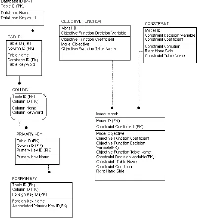
constraints. Figure 6.5 shows the new system catalog with the three new auxiliary

components included– the OBJECTIVE FUNCTION component, the CONSTRAINT

component, and the MODEL MATCH component. We call this new system catalog the

(50)

41 (Note: AS in Figure 5.1, the Associated Primary Key is the Primary Key ID inherited from the Primary Key

table and renamed)

Figure 6.5: The auxiliary catalog including the new OBJECTIVE FUNCTION,

(51)

42

The auxiliary catalog includes the following additional information:

• The OBJECTIVE FUNCTIONtable:

This table contains a unique identifier for each model that holds an objective function

(Model ID), and a unique identifier for each database table column that represents a decision variable in an objective function (Objective Function Decision Variable). These columns uniquely associate a corresponding objective function coefficient

(Objective Function Coefficient), model objective (Model Objective), and name of the objective function table (Objective Function Table Name)with its ID value.

Therefore, after the system catalog is defined and a table containing relational

information about the database tables is generated (Ref. Table 5.1), the columns in the

table are queried in such a way as to identify the column names that identify the

Objective Function Decision Variable(s), Objective Function Coefficient(s), and

Objective Function Table Name after which the column names are inserted into the

OBJECTIVE FUNCTION table according to their respective categories. Note here

that the Objective Function Decision Variable column in the OBJECTIVE

FUNCTION table is synonymous with, and an alias for, the Column Name column in the COLUMN table. The Column Name column is defined in the OBJECTIVE FUNCTION table through the PRIMARY KEY table as the Objective Function Decision Variable column. The user provides the Model ID that uniquely identifies each model. In addition, the Model Objective column is defined by the user as either a Minimization objective or a Maximization objective with the Minimization objective

(52)

43

FUNCTION auxiliary component is defined through the Model ID, Objective Function Decision Variable, Objective Function Coefficient, Model Objective, and the Objective Function Table Name.

• The CONSTRAINTtable:

This table contains a unique identifier for each model that holds constraint (Model ID), a unique identifier for each database table column that represents a decision variable in a constraint (Constraint Decision Variable), and a unique identifier for each database table column that represents a coefficient in the constraint (Constraint Coefficient). These columns uniquely associate a corresponding constraint condition associated with the constraint (Constraint Condition), right hand side constant in the constraint (Right Hand Side), and name of the constraint table (Constraint Table Name) with its ID value. Taken together, they uniquely identify a constraint.

Therefore, after the objective function table is defined, it is queried for to define the

Model ID. In addition, the information that was queried to define it is again queried in such a way as to identify the column names representing the Constraint Decision Variable, Constraint Coefficient, Right Hand Side constant, and the Constraint Table Name. The names are then inserted into the auxiliary component according to their respective categories. The Constraint Condition is defined by the user as either Greater-Than/Equal-To (GE) (the default), Equal-To (EQ), or Less-Than/Equal-To

(LE). Subsequently, the CONSTRAINT auxiliary component is defined through the

(53)

44

• The MODEL MATCHtable:

This table contains a unique identifier for each model that holds constraint (Model ID), and a unique identifier for each database table column that represents a

coefficient in a constraint (Constraint Coefficient). These columns uniquely associate a corresponding model objective (Model Objective), objective function coefficient (Objective Function Coefficient), decision variable in an objective function (Objective Function Decision Variable), the name of the table that holds the objective function data (Objective Function Table Name), decision variable in a constraint (Constraint Decision Variable), the name of the table that holds the constraint data (Constraint Table Name), the constraint condition associated with the constraint (Constraint Condition), and the right hand side constant in the constraint (Right Hand Side) with their ID values. Taken together, they uniquely identify a linear programming model.

Therefore, after the objective function and constraint tables are defined, they are

queried in such a way as to identify the column names representing a particular Model ID, Constraint Coefficient, Model Objective, Objective Function Coefficient,

Objective Function Decision Variable, Objective Function Table Name, Constraint Decision Variable, Constraint Table Name, Constraint Condition, and Right Hand Side constant. The names are then inserted into the auxiliary component according to their respective categories. Subsequently, the MODEL MATCH auxiliary

component is defined through the Model ID, Constraint Coefficient, Model Objective,

Objective Function Coefficient, Objective Function Decision Variable, Objective Function Table Name, Constraint Decision Variable, Constraint Table Name,

(54)

45 The following is an illustration of how the auxiliary components are defined including a

restatement of the preliminary actions:

Action 1. Define the original system catalog. Section 5.1 explains how this is done, the

results of which can be found in Figures 5.4 (a) and 5.4 (b).

Action 2. Highlight relational information about the database. Section 5.2 explains how this

is done, the results of which can be found in Table 5.1.

Action 3. Define the auxiliary components. At this point, the reader may find it helpful to

review sections 6.1 – 6.3, and Figure 6.2 in particular, for background information.

A. The OBJECTIVE FUNCTION table:

1. Define the model ID and insert it into the Model ID column. In this case the

Model ID is defined as “1”.

2. Identify the name of the column that represents the Objective Function Decision Variable by identifying, in Table 5.1, the primary key in the owned database table, and inserting the result, the column named “Viewership Type”,

into the Objective Function Decision Variable column.

(55)

46 table, and inserting the result, the column named “Viewership Cost”, into the

Objective Function Coefficient column.

4. Define the Model Objective as “Minimization” and insert it into the Model Objective column.

5. Identify the column that represents the Objective Function Table Name that corresponds to the Objective Function Decision Variable and Objective Function Coefficients by identifying this association, in Table 5.1. Insert the result, the table named “Cost_Data” into the Objective Function Table Name

column.

B. The CONSTRAINT table:

1. Identify the column that represents the model ID by extracting it from the

OBJECTIVE FUNCTION table, and insert it into the Model ID column. The result, “1”, is inserted into the Model ID column.

2. Identify the name of the column that represents the Constraint Decision Variable by identifying, in Table 5.1, the primary key in the dependent table, and inserting the result, the column named “Viewership Type”, into the

Constraint Decision Variable column.

3. Identify the name of the column(s) that represent the Constraint Coefficient(s) and Right Hand Side constant(s) by identifying, in Table 5.1 and in the

(56)

47 “Range” or a “Capacity” type. A “Range” data type is one that does not

inherently place operational limits on a system, such that altering the data

doesn’t fundamentally alter a system. Such a data type, if used in a constraint,

is viewed as a left side coefficient. A “Capacity” data type on the other hand,

inherently places operational limits on the system such that the only way to

alter the data and have the system remain valid is to alter the system. Such a

data type, if used in a constraint, is viewed as a right hand side coefficient.

Therefore, in our example, the results of the query used to identify the name

of the column(s) that represent the Constraint Coefficient(s) and Right Hand Side constant(s) are as follows: the columns named “Female Viewership” and “Male Viewership”, which are inserted into the Constraint Coefficient

column(s), and the “Viewership Requirement” column which is inserted into

the Right Hand Side column.

4. Define the Constraint Condition as Greater-Than/Equal-To (“GE”), and insert it into the Constraint Condition column.

C. The MODEL MATCH table:

1. Identify the column that represents the model ID by extracting it from the

OBJECTIVE FUNCTION table, and insert it into the Model ID column. The result, “1”, is inserted into the Model ID column.

2. Identify the following columns: the Constraint Coefficient, Model Objective,

Objective Function Coefficient, Objective Function Decision Variable,

(57)

48

Table Name, Constraint Condition, Right Hand Side by querying the

OBJECTIVE FUNCTION and CONSTRAINT tables based on the

definition of the Model ID column.

These actions prompt the changes to the auxiliary component tables of the auxiliary system

catalog that are shown in Figure A.1 in the Appendix.

Once the auxiliary system catalog components have been defined, the data that are identified

in the component definitions are extracted from a data table using in order to formulate a

linear programming model based on a given problem definition. Therefore, using the defined

auxiliary components, the following problem definition, and the resulting data held in Tables

6.1 and 6.2, we insert into our linear programming model data table, the data from Tables 6.1

and 6.2 according to how the model is defined in the auxiliary components. Table 6.3 in the

shows a linear programming model generated from the database after the model information

has been inserted into the auxiliary system catalog. We will show, in detail, how this table

(58)

49 Problem Definition

(59)

50

Viewership Type Cost

Comedy $50,000,000

Football $100,000,000

Table 6.1: Example model data in database table Cost_Data.

Viewership Type Female

Viewership

Male

Viewership

Requirement

Comedy 7,000,000 2,000,000 28,000,000

Football 2,000,000 12,000,000 24,000,000

Table 6.2: Example model data in database table Demographics.

Model Objective Objective Function Coefficient Objective Function Decision Variable Constraint Coefficient 1 Constraint Coefficient 2 Constraint Decision Variable Constraint Condition Right Hand Side

Minimization 50000000 Comedy 2000000 7000000 Comedy GE 28000000

100000000 Football 12000000 2000000 Football GE 24000000

(60)

51 Table 6.3 translates into the following linear programming model, shown below in Figure

6.6.

Minimize z = 50000000×1 + 100000000×2 Subject to 7000000×1 + 2000000×2 ≥ 28000000 2000000×1 + 12000000×2 ≤ 24000000

Figure 6.6: Example linear programming model formulation.

Here we show, step-by-step, how each column of Table 6.3 was created for this example. In

general, the queries and the modules that we used to execute each step can be found in the

Appendix section, along with the results of the execution of each step. The steps are as

follows:

Step 1. Create the LP Model Extraction Table Structure

A. A query is developed that creates a table called LP Model Extraction

Table. This table holds the columns Model Objective, Objective Function Coefficient, Objective Function Decision Variable, Constraint Coefficient

(1 through N) where N is the total number of records in the Constraint Coefficient column of the Constraint Table, the Constraint Decision Variable, Constraint Condition, and Right Hand Side.

B. The columns were formatted as follows:

(61)

52 - Objective Function Coefficient as a numeric column.

- Objective Function Decision Variable as a text column with a maximum spacing of 32 characters.

- Constraint Coefficient (1 through N) as a numeric column. - Constraint Decision Variable as a text column with a maximum

spacing of 32 characters.

- Constraint Condition as a text column with maximum spacing of 32 characters.

- Right Hand Side as a numeric column. The results of Step 1 are shown below in Table 6.4.

Model Objective Objective Function Coefficient Objective Function Decision Variable Constraint Coefficient 1 Constraint Coefficient 2 Constraint Decision Variable Constraint Condition Right Hand Side

Table 6.4: LP Model Extraction Table after Step 1.

Step 2. Populate the Model Objective Column

A query is developed that inserts into the LP Model Extraction Table, data selected