IC Design Analysis, Optimization and Reuse via Machine Learning.

(1)

ABSTRACT

QI, WEIYI. IC Design Analysis, Optimization and Reuse via Machine Learning. (Under the direction of Dr. Paul D. Franzon.)

Since the introduction of the Moore’s law in 1965, the integrated circuit industry has

successfully managed over 50 years of exponential growth in design complexity and the

transistor number has grown from thousands to billions on a single chip. Electronic design

automation (EDA) tools are among the biggest factors that keep this growth trend and lead

to the developments of cost- and energy- efficient robust electronic circuits and systems.

As technology node continues to scale down, the traditional EDA-based design

method-ology is challenged from many aspects. Firstly, the growing design complexity results in a

significant increase in the computational cost and human labor for conducting thorough

design analysis and optimization, both of which are keys to IC design successes. Secondly,

the sophisticated underlying physics of advanced technology nodes make the modeling

capability of the EDA tools questionable. In fact, most of the failures observed in

quali-fication tests are direct results from such modeling issues, examples include mistuned

analog circuits, signal timing errors, reliability problems, and crosstalk. The qualification

failures in fabricated chips imply additional rounds of designs, known asdesign respinsand it requires more efficient and reliable EDA tools to design high-yield circuits and systems

aiming at the maximum utilization of the new technology and potentially eliminate the

need for design respins.

In this work, we demonstrate how machine learning helps to alleviate the bottlenecks

mentioned above. We particularly focus on the enhancement of simulation-based

method-ology for efficient design analysis, modeling, optimization, and yield estimation.

(2)

simulation-based design methodology is to harness the statistical models’ capability of extracting

information from the limited data set and make fast predictions about unobserved designs

as well as accurately quantify the prediction uncertainty. The model can be used either as a

direct surrogate of the expensive simulator or as a guide for the design decision-making

process.

In this work, we demonstrate the efficacy of the proposed methodology through several

circuit and system designs. Examples include the calibration of reliability-related

degrada-tions in mixed-signal circuits, fast configuradegrada-tions of the physical design flow, automatic

analog circuit optimization and intellectual property (IP) reuse, and yield estimation of

(3)

(4)

IC Design Analysis, Optimization and Reuse via Machine Learning

by Weiyi Qi

A dissertation submitted to the Graduate Faculty of North Carolina State University

in partial fulfillment of the requirements for the Degree of

Doctor of Philosophy

Electrical Engineering

Raleigh, North Carolina

2017

APPROVED BY:

Dr. Brian A. Floyd Dr. William R. Davis

(5)

DEDICATION

To my parents, Baoxian Hao and Shuying Qi, who have taught me the virtues of

(6)

BIOGRAPHY

Weiyi Qi was born in Xingtai, Hebei Province, China on December 27th, 1989. He received

his Bachelor of Science (B.S.) degree in Electrical and Information Engineering from Dalian

Jiaotong University in 2011, and the Master of Science (M.S.) degree in Electrical Engineering

from North Carolina State University in 2013.

Weiyi joined Dr. Paul Franzon’s research group in February 2012, when he started his

Ph.D. research on surrogate modeling for the acceleration of computationally expensive

circuit simulation as a part of the self-HEALing mixed-signal Integrated Circuits (HEALICs)

project funded by DARPA. In 2016, he became a student member of the Center for Advanced

Electronics through Machine Learning (CAEML), with a research focus on machine learning

aided design analysis, optimization, and reuse of analog intellectual properties.

(7)

ACKNOWLEDGEMENTS

No man is an island, entire of itself.

John Donne

First of all, I would like to thank my advisor, Dr. Paul D. Franzon, for providing me with

such incredible research and study opportunities. Dr. Franzon gives me the freedom to

explore my ideas and the help when I am in the face of obstacles. His insights, enthusiasm,

supports, and encouragements inspire me and guide me through this wonderful journey.

To me, Dr. Franzon is more than an advisor in academics, but in life, too. Those wise words

and deeds will become invaluable assets for me, forever.

I want to express my deepest appreciation to Dr. Floyd, who serves as a role model

with his attitude and integrity to the academics; Dr. Davis, who gives me inspirations and

suggestions through many of our discussions; and Dr. Vatsavai, from whom I acquired my

rudimentary knowledge of machine learning and data mining. Also, my sincere gratitude

goes to them for serving as my committee members.

I am also grateful to the following people and organizations, without whom I could

not have made this accomplishment. These include Dr. Min Kang, who exposed me to the

beauty of math and probability; Dr. Steve Lipa, whose help and advice are crucial at the

beginning of my Ph.D. study; and my group fellows, Zhuo Yan, Jianchen Hu, Zhenqian

Zhang, Wenxu Zhao, Weifu Li, Jong Beom Park, Josh Schabel, Zhao Wang, Nazia Zannat,

Lee Baker, Kirti Bhanushali, Yi Wang, and Bowen Li, who have made special pieces of

the beautiful memory of the past years. My courteous acknowledgment goes to DARPA,

Raytheon, the CAEML center, and NSF for the supports of my research projects. I would

also like to express my best feelings to the Samsung Device Lab and my colleagues for their

(8)

Finally, I would like to give my most sincere gratefulness to my dear family. Oceans

(9)

LIST OF TABLES

Table 1.1 Comparative Study of Analog Optimization Techniques . . . 12

Table 1.2 Comparative analysis of Monte Carlo techniques . . . 23

Table 3.1 VCDL Inputs and Output Summary . . . 56

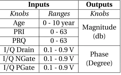
Table 3.2 Phase Rotator Inputs and Outputs Summary . . . 59

Table 3.3 CORTEX Physical Design Parameter Summary . . . 66

Table 3.4 Results of iteration 1 . . . 69

Table 3.5 Physical Design Iterations . . . 70

Table 5.1 Model parameter settings . . . 116

Table 5.2 Prediction Speed Comparison (107_{predictions) . . . 117}

Table 5.3 Cantilever Parameter Distribution . . . 117

Table 5.4 Prediction accuracy comparison . . . 118

Table 5.5 Cantilever performance comparison . . . 123

(13)

LIST OF FIGURES

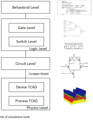
Figure 1.1 Levels of simulation tools . . . 4

Figure 1.2 Illustration of Surrogate Modeling . . . 6

Figure 1.3 Analog optimization tool categories . . . 12

Figure 1.4 General reliability design procedure . . . 14

Figure 1.5 General reliability design procedure . . . 23

Figure 2.1 Key surrogate modeling stages . . . 29

Figure 2.2 A 2-D example of latin hypercube sampling (10 points) . . . 32

Figure 2.3 Handling nonlinear data with Linear Regression, created with the scikit-learn package[109]. . . 39

Figure 2.4 Handling nonlinear data with Polynomial Regression, created with scikit-learn package . . . 40

Figure 2.5 Regression using RBF model, created with SciPy package[63]. . . 42

Figure 2.6 Under-fitting, desirable model, and over-fitting. Created with the scikit-learn package . . . 44

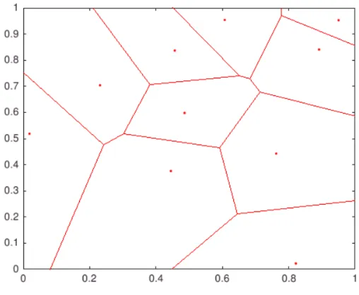
Figure 2.7 Regularization for over-fitting. Created with the scikit-learn package 45 Figure 2.8 2-D example of Voronoi tessellation . . . 49

Figure 3.1 Block diagram of the VCDL test infrastructure . . . 55

Figure 3.2 The parallel simulation flow . . . 57

Figure 3.3 Contour Plot of the VCDL Model . . . 58

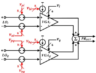
Figure 3.4 Block diagram the phase rotator design . . . 60

Figure 3.5 The point-by-point simulation of the phase rotator phase response surface . . . 61

Figure 3.6 Direct modeling lead to a smoothed response surface of the phase rotator phase . . . 62

Figure 3.7 LOLA-Voronoi HDMR Modeling Flow . . . 63

Figure 3.8 The Phase Rotator Phase Response Model . . . 64

Figure 3.9 The Phase Rotator Magnitude Response Model . . . 64

Figure 3.10 The Macro-Structure of the CORTEX SoC Platform . . . 66

Figure 3.11 Trivial Effects of sinkMaxTran and maxSkew on Congestion . . . 67

Figure 3.12 Trivial Effects of sinkMaxTran and maxSkew on Setup slack . . . 68

Figure 3.13 Significant Effects of sinkMaxTran and maxSkew on Hold slack . . . . 68

Figure 3.14 Congestion vs. Layers (CLKper=10, density=0.6) . . . 69

Figure 3.15 Final design details . . . 71

Figure 3.16 Snapshot of the final routed design . . . 72

Figure 4.1 Proposed work flow . . . 76

(14)

Figure 4.3 Design goal distribution and correlation . . . 96

Figure 4.4 Balun optimization comparison . . . 97

Figure 4.5 (a) Manual balun design in 8XP; (b) Balun redesign in 8XP; (c) Balun reuse in 9HP . . . 98

Figure 4.6 Power amplifier schematics . . . 99

Figure 4.7 PA Design parameter screening . . . 100

Figure 4.8 PA optimization comparison . . . 101

Figure 4.9 (a) Manual PA Design in 8XP; (b) PA redesign in 8XP; (c) PA reuse in 9HP; (d) Result comparisons (Simulated at 80GHz) . . . 102

Figure 5.1 Illustration of the symbolic regression tree . . . 107

Figure 5.2 Sample distribution of iteration 1, 2, 4, and 8 . . . 121

Figure 5.3 Convergence plot of the Cantilever example . . . 122

Figure 5.4 SRAM schematics . . . 124

(15)

CHAPTER

1 INTRODUCTION

Integrated circuit (IC) designs depend on sophisticated parameter tuning and decision

making with the help of software tools, commonly known as the computer aided design

(CAD) or electronic design automation (EDA) tools. Over the past few decades, the

ad-vancements in computing power has given rise to an explosion in the capability of the EDA

software that guarantees the IC industry to keep up with the Moore’s law[105]. Among all

the EDA tools, simulation is the key to drive the development of low-cost, safe and robust

(16)

obscure the lower level details in order to trade off the overall performances of simulation

speed and accuracy[19]. From bottom to top, these abstraction levels include:

1. Physics level:

At device physics level, the goal is to build technology CAD (TCAD) models of the

semiconductor fabrication and device operations. The former one is calledprocess TCAD, while the latter device TCAD [78]. Both process and device TCAD models have high fidelity at the physics level, but it is too expensive to be used directly in

circuit simulations, therefore, TCAD also produces compact models that capture the

electrical behavior as mathematical equations without resorting to the underlying

physics. A well known example of compact models is the SPICE transistor model.

2. Circuit level:

Circuit level simulators analyze transistors, wires, capacitors, resistors, and their

interconnectivity[19], then model the schematics or layout behaviors by solving

dif-ferential linear equations formed from operation principles such as the Kirchhoff’s

laws (KVL and KCL). Circuit level simulators produces accurate waveforms that

resem-bles the real world operation. Accurate as it is, this technique can be computationally

intensive, especially for larger designs, so it is usually used in the most critical blocks

of a system, often the analog and mixed-signal subsections.

3. Logic level:

Logic level simulations steer away from the continuous data and attempt to abstract

the behavior at the boolean level (1/0/X). Further assumptions are made to facilitate

(17)

At a lower logic level, each transistor is treated as a switch that has either 1 (on) or 0

(off ) states, this is called the switch-level simulation; at a a higher logic level, groups

of transistors, resistors, and capacitors are further abstracted to logic gates, flip-flops,

XOR, for instance, this is known as the gate-level simulations. Logic level simulators

makes it possible to efficiently study the behaviors of more complicated systems.

4. Behavioral level:

Behavioral level simulations are also known as the functional level simulations. These

simulations model the architectural operations and are accurate at cycle- or

interface-level[78]. Behavioral level simulations are useful as they provide an overall picture of

how design and control flows work and interact, thus making rapid prototyping and

path-finding possible. But as most details are hidden, behavioral simulations could

easily lead to infeasible designs or tedious lower-level implementations.

By representing the simulation levels as a stack structure, an illustration is shown in

Figure 1.1 below1_.

1.1 Motivation

Hierarchical simulation abstraction levels trade off simulation speed and accuracy by

gradually hiding away the details from lower levels. Still, simulation-based designs are

reaching their bottlenecks as the IC design complexity grows. On one hand, the overhead in

computational cost and the simulation speed has increased dramatically; on the other hand,

the simulation accuracy and model capability are severely challenged by the complicated

(18)

(19)

circuit behaviors. As a consequence, the design process based on simulation tools become

extremely inefficient, and there is an urgent need to bridge the different levels and create

models that are fast enough but without severely impair the accuracy.

We can achieve this goal using surrogate models, also known as meta-models or

re-sponse surface models (RSM)2. Such models seek to approximate the real and expensive simulation responses and make predictions of the unseen by augmenting the information

given by a limited number of observed data. A fundamental assumption of this approach is

that the surrogate models are orders of magnitudes faster while still being accurate enough

to use[33].

We show the general idea of surrogate models in Figure 1.2. Essentially, surrogate models

stems from the family of predictive models in supervised machine learning. The main

distinction of surrogate models from other supervised machine learning models is the

ability to cope with the scarcity of training data. Generally speaking, surrogate models

obscure the underlying physics and seek to represent the input-output relationships using

a "learned " mapping function. The input space is strategically sampled so as to minimize

the data consumption and improve the modeling efficiency while still ensuring enough

information being retrieved regarding the underlying "true" relation.

Surrogate models proves to be useful in various fields, such as aerodynamics[71],

struc-tural reliability[38], mechanical designs[120], I/O circuits[142], semiconductor device

mod-eling[137], microwave circuit optimiation[6],etc.

In this work, we try to harness the advantages of speed-accuracy trade-off associated

with surrogate models to tackle design exploration, optimization, and yield analysis of

2_{In the rest of this paper, we will use the terms "surrogate models", "predictive models", "metamodels"}

(20)

Figure 1.2Illustration of Surrogate Modeling

IC and system designs. In particular, this dissertation emphasizes on automatic analog

intellectual property (IP) reuse and reliability analysis of rare-event circuit failures. In the

rest of this chapter, we will conduct a literature review of the existing works on these two

topics. For the sake of brevity, interested readers are referred to[102]for a discussion on how

predictive models have been used in other EDA fields, such as circuit level and architecture

level path-findings.

1.2 Related Works I: Analog Optimization and IP Reuse

In recent years, considerable research efforts in both academic and industrial communities

are devoted to the computer-aided solutions of designing analog circuits. Aiming at full

functionality, these tools often cover the entire workflow of analog synthesis, including

topology selection, performance optimization, and layout generation. In this work, however,

(21)

consists re-optimization in the same process nodes (calledre-design) and migration to new nodes (orreuse). Note that, by "reuse", we assume the identical topology is maintained in both cases. We will discuss the most significant efforts in related fields in the next

sec-tions. Briefly speaking, these techniques can be broadly categorized into knowledge-based

approaches and optimization-based approaches[86].

1.2.1 Knowledge-based approaches

The main purpose of knowledge-based approaches is to encapsulate the designers’

knowl-edge, whether it be building a pre-design plan with design equations and a design strategy

that produces the component sizing[7]or representing the design procedure as a set of

flowcharts and converting the intrinsic dependencies of device parameters into graphs[46]

to guide the design and optimization, hence two main groups of knowledge-based

ap-proaches can be found in literature: design plan driven methods and operating point driven

methods.

A) Design Plan Driven

This method characterizes a complete design plan that describes how the circuit

com-ponents need be sized to reach the design specifications. Analytical or empirical equations

are often used to explore the design space and trade off performances.

Representatives of design plan driven knowledge-based approaches includes[24, 30, 48,

52, 79]. The main advantage of this method is that once the execution plan is defined, the

speed for sizing is very efficient and the solution quality only depends on the evaluator’s

accuracy. However, there are two significant drawbacks: (1) the overhead of defining and

(22)

topolo-gies[48]. Moreover, though satisfying the design specifications, there is no guarantee in

finding the optimum solution using the design plan drive approaches[89].

B) Operating Point Driven

More recently, works on the knowledge-aware analog synthesis and IP reuse are

pro-posed in[57, 59, 60]. The essential foundation of this approach is on the operating-point

driven formulation of analog CAD[46]and derived from traditional handcrafted analog

cir-cuit design method, where the operating points are calculated first, and then the attributes

(such as aspect ratios) can be determined from the operating points by inverting the

ana-lytic equations. The CAIRO+platform[56]uses bipartite graphs to express the operating

point dependency. Together with a group of operators for inverting the BSIM compact

models, this framework is able to determine the transistor aspect ratios. The advantage

of such knowledge-aware operating point drive approach is that designer can maintain

insights of the impacts of design variables (voltages, currents) on performances thus

en-hance the efficiency of circuit reuse in the same technology. However, the inverse operators

need to be updated or re-developed to support different compact models[55]. Therefore,

it is less generally applicable and also results in a long preparation time, similar to other

knowledge-based approaches.

1.2.2 Optimization-based approaches

Optimization-based approaches translate the analog optimization and IP reuse problem

to the minimization (or maximization) of objective functions, which is then solved by

numerical methods or optimization algorithms. Instead of using design plans, optimization

(23)

till the design meets particular specifications. Nowadays, optimization-based approaches

are widely accepted and used[117], mainly due to the automaticity characteristic that keeps

a human out of the loop. To form this automatic loop, optimization algorithms are paired

with performance evaluators that evaluate the quality of the design. Three main types of

performance evaluator are used,i.e.analytical equation, circuit simulator and behavioral models[7].

A) Analytical equations

The analytical equations are derived either manually or with automated tools. Relevant

works include[11, 40, 42, 49, 69, 88, 91, 95, 107]. Analytical equations are conceptually

mathematical representations of the circuit blocks and are known for their short evaluation

time which is a significant advantage in design space exploration and performance

opti-mization. However, despite recent advances in symbolic circuit analysis[87], not all design

characteristics are captured with equations. One reason is that there is a dilemma that

closed-form analytical equations call for simplifications, which in turn results in inaccuracy

and incompleteness in analytic equations. Using inaccurate or incomplete evaluators will

impose severe restrictions to the final optimized circuit performance.

Asides from the methods above,[1, 22]proposed to express analog designs and

opti-mization tasks in posynomial forms. As the posynomial expressions are intrinsically convex,

the global solution can always be found regardless of where the starting point is[11], thus

can be solved efficiently with geometric programming techniques. Nevertheless,

reformu-lating accurate device models in posynomial forms is challenging, as the author indicated:

“performance specifications and objectives that can be handled are far more restricted than

(24)

B) Circuit simulator

This method incorporates circuit simulators in the optimization loop to evaluate the

performances.[72, 73, 84, 86, 95, 106, 110, 127]cover various uses of circuit simulators as

performance evaluators. Clear advantages over the equation-based approach are (1) the

evaluation accuracy and flexibility for different kinds of analog design blocks, and (2) it

also allows reliability analysis such as the Monte Carlo and aging degradation analysis[112],

both with minimal setup time.

However, in spite of the clear advantages of simulator-in-the-loop methods, the

compu-tational cost of circuit simulators prohibits its further adaptability, as common optimization

algorithms (such as evolutionary algorithms) on analog circuit requires hundreds or even

thousands of function evaluations to achieve optimal designs[84].

C) Behavioral models

To address the accuracy issue in equation models and computational drawback in

the simulator-in-loop method, learning-based methods provide a promising solution to

enhance the efficiency of optimization-based methodology. The idea is to build behavioral

models from a set of training data which are sampled by executing circuit or system

simu-lations and then use machine learning techniques to model the input-output resimu-lationship

mapping. In[85], Liuet al.proposed data-mining based macro-modeling techniques for large analog design space exploration, and demonstrated the clear optimization efficiency.

Recent works regarding behavioral model-based techniques on analog optimization are

presented in[3, 23, 85, 133]. For example,[3]used neural-fuzzy models with

evolution-ary optimization strategies and[23]developed support vector machine (SVM) models to

(25)

macro-model was trained to be used for analog circuit synthesis, the macro-model can substitute for full

SPICE simulation and the inclusion of design rules for sizing and operating points also

substantially shrank the design space and ensured correct functionality.

Behavioral models are comparable to full circuit simulations in accuracy and have the

speed on a par with analytic equations. This characteristic makes it particularly favorable

for optimization-based approaches[133]. Successful applications of model-based analysis

have been demonstrated in[135, 137, 138, 142], which shows that behavioral models can

also characterize circuit variability and reliability to improve design robustness. Moreover,

in the case of analog IP reuse, behavioral models can additionally help alleviate the IP

bottleneck, in which surrogate models act as substitutes of the detailed schematics or

layouts.

To train such accurate predictive models, a set of training samples from the high fidelity

evaluators, such as SPICE simulators, are required. The number of training samples reflects

the trade-off between computational cost and model performance: for more complicated

circuits with higher dimensionality, the computational cost of maintaining a desirable

accuracy increases exponentially with the number of free parameters. This phenomenon is

known as “the curse of high dimensionality”[33].

1.2.3 Analog Optimization and IP Reuse Summary

The summarization of different analog optimization and IP reuse techniques in presented

Figure 1.3 with a comparative analysis in Table 1.1. In the table, "X", "-", and "Ø" stand for

"good", "moderate", and "bad", respectively. From this table, we notice that model-based

(26)

Figure 1.3Analog optimization tool categories

Table 1.1Comparative Study of Analog Optimization Techniques

Knowledge-based Optimization-based

Design Plan OP Driven Equation Simulation Surrogate Model

Setup Time X X Manual: X

Tool: - d

-Design Time _Ø _Ø _Ø X

-Accuracy - - - Ø

(27)

1.3 Related Works II: Yield Estimation

Yield estimation is also known as reliability analysis. It is an essential part of almost any

aspect of engineering design. Specifically, for IC designs, the designers need to take into

consideration of two kinds of variations: the variations during manufacturing and the

uncertainty during operations. The former one is known as the process variations (P) while

the latter includes voltage (V) and temperature (T). Reliability analysis for IC design thus

requires the identification of chances that the system enters a suboptimal situation under

PVT variations, or equivalently estimating the probability of failure (αf).

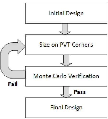
Reliability aware design is critical in all IC design tasks, including radio-frequency (RF),

analog, mixed-signal circuits, I/O designs, and memory, etc. The reliability aware design

flow usually consists of corner-based design followed by a Monte Carlo verification step[93],

with the flow diagram shown in Figure 1.4:

However, there are two main drawbacks associated with this procedure: corner models,

despite their appealing speed, usually lead to pessimistic designs that cause the over-design

problem; while the Monte Carlo step gives a better estimation of the final yield, but at the

cost of lengthy simulation and massive computational power.

Many alternatives are proposed in the literature, including sophisticated designs of

experiments (DoE), improved statistical estimation, and surrogate model enabled Monte

Carlo techniques. In the next sections, we will first discuss how crude Monte Carlo method

works and its bottleneck in estimating rare events, and then conduct a brief review of the

(28)

Figure 1.4General reliability design procedure

1.3.1 Crude Monte Carlo

Due to the black-box nature of the distribution of performance metrics, designers need to

rely on simulations to assess the design failure probability, which is typically done using the

Monte Carlo approach. Essentially, Monte Carlo method involves repeating the simulation

many times with different design or environment parameter settings and approximating

the failure rate by countering the observed failures against the total number of simulations

conducted.

Consider ad-dimensional random vectorX distributed according toPX with a

prob-ability density function (PDF)pX, these are the inputs (design parameters and/or PVT)

(29)

for simplicity, we only consider f as a scalar function, but it can be readily generalized to multiple-output cases. Suppose the system fails whenf (X)>u, whereu ∈Ris called the thresholddetermined from the design specifications. The failure region is therefore:

Γ ={x∈X|f(x)>u}. (1.1)

And the probability of failure:

αf =PX(Γ) =

Z

Γ

pX(x)d x =

Z

X

1_Γ(X)pX(x)d x. (1.2)

where 1_Γ(X)is an indicator function:

1_Γ(X) =

 



1 :x∈Γ 0 :x∈/Γ

(1.3)

With crude Monte Carlo,α_f is approximated as:

ˆ αf =

1

N N

X

i=1

1_Γ(X). (1.4)

According to the law of large numbers[58], this estimation is an unbiased estimate that

converges to the real probability as N increases. One usually use the relative error to quantify

the estimation efficiency[96]. The relative error (also known as the relative deviation) is:

R E(αˆ_f) = σαfˆ

E(αˆ_f). (1.5)

(30)

of proportion, we haveσαˆf =

Ç_αf_ˆ ₍ 1−ˆαf)

N , therefore,

R E(αˆf) =

Ç_αf_ˆ ₍ 1−ˆαf)

N

σαˆf =

v u

t(1−αˆf) ˆ αfN

≈ v u

t 1

ˆ αfN

.

(1.6)

To illustrates the inefficiency of crude Monte Carlo method under computational budget

when estimating a small probability of failure, suppose the estimation calls for 10% relative

error, for estimating

a l p h a=10−3_{, the total sample number needed from a crude Monte Carlo simulation is:} 100

ˆ

αf =105.

Another intuitive view of the inefficiency is that most simulations are wasted because

they don’t catch the failure cases. Again, suppose we want to verifyα=10−3, on average, 1000 simulations are needed in order to catch a single failure simulation.

1.3.2 Efficient Monte Carlo techniques

Efficient reliability analysis for small probabilities of failure is indispensable when designing

robust circuits and systems and has drawn significant attentions from people with different

backgrounds. The approaches are usually sorted into three main categories[8]: geometric

approximation in the distribution space, variations of the Monte Carlo approach, and

surrogate model assisted methods. In this section, we will review the representative works

(31)

1.3.2.1 Geometric Approximation

Geometric approximation methods aim at approximating the contour of the failure region

(Γ) geometrically with simpler shapes ˆΓ. An approximation of the integration in Equation

(1.4) is:

ˆ

αf(G e o)=PX(Γˆ)

=

Z

X

1ˆ_Γ(X)pX(x)d x.

(1.7)

An apparent advantage of this approach is that once we form ˆΓ, no further evaluation

is needed to estimateαf as it is calculated using probability calculus. In other words, all

function evaluations or simulations are spent in finding the contour approximation.

An example of the geometric approximation is the first/second order reliability methods

(FORM/SORM) which are prevalent in structural safety literature[83]. The typical steps for

conducting FORM/SORM involves four steps:

(1)Input distribution transformation:The input distribution is mapped fromPX into a standard multivariate normal distributionV.

(2)Search for the Most Probable Point (MPP) in V :The MPP is the point on the failure boundary that is closest to the distribution center (So it has the highest probability of failure

among all the points residing on the failure boundary).

(3)Geometrically approximating the failure boundary:This step can be regarded as a first-/second-order expansion of the failure boundary with respect to the MPP, in which

(32)

the true failure region.

(4)Calculating the probability of failure:With the approximated failure boundary, the calculation of failure probability inV is simply done using the standard normal pdf.

It is apparent that the success of this category of methods depends on the contour

approximation quality. Several factors limit this quality, however, such as the nonlinear

transformation in Step (1) or multimodality issues, where more than one MPP exists.

1.3.2.2 Variants of Monte Carlo Method

Many variants are proposed to overcome the inefficiency of crude Monte Carlo method.

Among all the techniques, we will discuss three most representative ones, includingquasi Monte Carlo methods,importance sampling, andsubset simulation.

(1)Quasi Monte Carlo methods

These methods are also known as low-discrepancy sampling and base themselves on

variance reduction techniques[116]. The main idea is to generate samples in the

distribu-tion space with a better spread, so as to achieve the same accuracy of crude Monte Carlo

simulation with fewer samples. For example,[50]and[27]demonstrated the use of Latin

Hypercube sampling and stratified sampling respectively. However, it doesn’t solve the root

problem regarding Monte Carlo simulation: for a one-in-a-billion failure case, one still

needs, on average, 1 billion simulations to capture a single failure point.

(2)Importance sampling

The core of importance sampling is to strategically modify the sampling distribution so

that the probability density function (PDF) can be shifted towards the failure region. As a

(33)

Leth be a proposal PDF, the failure probabilityαis written as:

αf =

Z

X

1_Γ(X)pX(x)d x

=

Z

X

1_Γ(X)pX(x)

h(x) h(x)d x

=Eh

1_Γ(X)pX(x) h(x)

.

(1.8)

whereEhdenotes the expectation with respect to the proposal PDFh. Now, with

impor-tance sampling:

ˆ αf(I S)=

1

N

X

i=1

N1_ΓpX(x)

h(x) . (1.9)

The primary challenge for importance sampling is to effectively determine the optimal

proposal density functionh∗_{. According to}_[₉₆_]_{, this optimal is reached by minimizing the} variance of ˆα_f₍_{I S}₎:

h∗=arg minV a r(αˆf(I S)) =

1_Γ(X)pX

R

X1Γ(X)pXd x

=1Γ(X)pX

α . (1.10)

Notice thath∗_{in turn depends on the unknown failure region}_Γ_{, so the minimization} problem is ill-posed. To overcome this dilemma,[116] introduced the adaptive

impor-tance sample technique that involves generating intermediate Monte Carlo simulations

with proposal densitieshi,i =1, ...,T to sequentially approachh∗, either parametrically or

non-parametrically. In parametric adaptive importance sampling, one uses a vector of

(34)

ap-proach, instead of estimating the density parameters, the density function itself is estimated,

such as with the Gaussian kernels[43]. In both methods, the quality of the approximation is

measured with the Kullback–Leibler divergence[96].

Importance sampling techniques is the state-of-the-art rare-event simulation algorithm

in lower dimensional cases. However, as dimensionality increases, finding good proposal

distribution functions becomes nontrivial, and therefore a screening step is necessary to

identify the most important features and reduce the dimensionality.

(3)Subset simulation

Instead of approximating the underlying distribution function, as with importance

sampling, subset simulation instead partitions the performance domain by dividing the

rare event into a series of nested less rare events, the failure probability is then a product of

the nested conditional probabilities.

Precisely, one builds a sequence of increasing thresholds_{ui}i=1,...,T , such that−∞< u1<u2<...<uT =u. This correspond to a decreasing sequence of failure regions{Γi}i=1,...,T,

whereX ⊇Γ1⊇Γ2⊇..._⊇Γ_T =Γ[83].

The probability of failure is therefore:

αf(SS)=PX(Γ)

=PX(Γ1) T−1 Y

t=1

PX(Γt+1|Γt)

=

T

Y

t=1

pt

(1.11)

For eachpt =PX(Γt+1|Γt), suppose we generate samples according toPX(.|Γt), then with

(35)

in subset simulation literature. In each iterationt, we keep the samples located inΓ_t₊₁and generate an i.i.d sample using the sequential Monte Carlo method[9].

Subset simulation uses the divide-and-conquer technique and efficiently decomposes

the complicated situation into a sequence of easier-to-solve problems. However, in each

decomposed step, even though the overall required number of samples is significantly

smaller than that of the crude Monte Carlo methods, the conditional probability is

usu-ally determined by Markov Chain Monte Carlo (MCMC) simulations that still requires a

relatively high simulation cost. This makes subset simulation unappealing characteristic

when handling expensive evaluations, such as radio-frequency circuits and electromagnetic

designs.

1.3.2.3 Surrogate model assisted methods

In the first part of related works, we have discussed the advantages of surrogate/behavioral

models for optimizing expensive simulation-based analog designs. Indeed, surrogate

mod-els also help Monte Carlo simulations: by modeling the expensive system with a

cheaper-to-evaluate surrogate, the reliability estimation is done either with a direct substitution or

guided by the surrogate.

When surrogate model is used as a direct substitution, it is called the response surface

Monte Carlo method. Earlier examples include[13, 29, 31], and some recent developments

are demonstrated in[39, 66, 139]. In[108]artificial neural network model is adopted, and

[54]utilizes the SVM model. The direct substitution method is a simple and straightforward

approach for incorporating surrogate models in the reliability estimation loop, but as with

(36)

results. Therefore, when handling higher dimensional or nonlinear response surfaces, the

performances of direct substitution is in doubt.

Instead of using surrogate models directly, one can also use the model to guide the

sampling steps. For example,[122]used a decision tree to block unnecessary simulations of

an SRAM cell, and[8]uses Gaussian process model for sequential Monte Carlo simulation. In

[9], Gaussian processes are incorporated in subset simulation, resulting in a technique called

theBayesian subset simulationthat avoids the cost of MCMC for conditional probability estimation at each step and instead use the information given by the Gaussian process

predictions. In[93], a symbolic regression model is trained to sort the simulation sample

sequence and perform data mining in the massive Monte Carlo samples.

1.3.3 Yield Analysis Summary

We summarize the categories of yield analysis techniques in Figure 1.5 and also present a

comparative study in Table 1.2. In the table, "XX" means extremely prohibitive, "X" and "Ø"

indicate bad and good, respectively, while blanks denotes "moderate" or hard to evaluate.

Again, we notice that model assisted Monte Carlo simulation is the most promising solution,

especially when computational resource is under tight budgets.

1.4 Disseration Organization

In the following chapters, we begin our discussion with an overview of the machine learning

and surrogate model fundamentals, including sampling plan, model constructions, and

(37)

Figure 1.5General reliability design procedure

Table 1.2Comparative analysis of Monte Carlo techniques

Crude MC

Quasi MC

FORM/ SORM

Importance Sampling

Subset Simulation

Direct Model

Model Assisted Computational

Cost XX X Ø Ø Ø

Estimation

Accuracy X X Ø

High

Dimensionality Ø X X X Ø X

Disjoint

Failure Region Ø Ø X Ø

(38)

design examples, including a voltage-controlled delay line (VCDL), a phase rotator, and a

physical design of the CORTEX processor. In Chapter 4, we present the automatic analog

design analysis, optimization, and reused flow with the core algorithm called Bayesian

optimization. We continue our discussion on how ensemble models enhance the efficient

yield estimation of SRAM circuits in Chapter 5. In the final chapter, a summary and an

outlook of future work are presented.

1.5 Research Contributions

The main contributions of this dissertation include:

1. Implemented a parallel model construction flow to facilitate the development of aging-induced degradation calibration algorithm.(Chapter 3)

Sequential surrogate modeling flow typically adds one new sample at each iteration,

in this parallel flow, we modified the sampling criteria so that more than one sample is

requested each round and implemented the multi-server parallel infrastructure to greatly

ex-pedite the model construction process. The flow is demonstrated with a voltage-controlled

delay line and a phase rotator design and is>10X speedup, compared with the original

flow in[141].

2. Proposed and implemented the High Dimensional Model Representation (HDMR) modeling flow for handling high-dimensionality in behavioral models.(Chapter 3)

When modeling the phase rotator problem, traditional predictive models tend to destroy

the desired response surface by smoothing out the nonlinear regions. We introduced the

(39)

of lower dimensional ones and was able to preserve the response surface trait to test the

robustness of the calibration algorithm.

3. Proposed and implemented an automatic flow for analog circuit design analysis, optimization, and intellectual property reuse.(Chapter 4)

Analog redesign and reuse between technology nodes are design-expertise intensive.

We advocate the use of Bayesian optimization along with Student-tprocesses to efficiently produce high-quality designs. Moreover, this is the first application of Student-tmodel based Bayesian optimization in engineering designs.

4. Improved the HSMC algorithm with ensemble models for the estimation of rare-event failures in SRAM.(Chapter 5)

We enhanced the high-sigma Monte Carlo (HSMC)[93]algorithm using ensemble

learn-ing models. The resulted algorithm proves to converge faster than the original one, and we

(40)

CHAPTER

2 SURROGATE MODEL FUNDAMENTALS

In this chapter, we will introduce the fundamental concepts in surrogate models, and lay

the foundation for in-depth discussions of different predictive modeling techniques along

with their applications in the follow-on chapters.

2.1 Introduction to Surrogate Modeling

Recall that the goal of surrogate modeling is to train a mapping function using limited

(41)

can be used as a surrogate to represent the original process. Precisely, suppose the original

expensive model is denoted asy =f(x), wherexis the input vector,f is the true function, andy is the output. We wish to "learn" an estimated function ˆf(x) +ε(x)of the original mapping from a small observed datasetDgenerated from f. This estimation contains two parts: ˆf (x)is the expected value from the surrogate model andε(x) quantifies the uncertainty of the estimation.

This is indeed a regression problem in the statistical learning realm, in which a good

paradigm for selecting the estimator ˆf is by solving the Tikhonov regularization prob-lem[113]:

min ˆ

f∈HZ( ˆ

f) = 1 Ns

Ns

X

i=1

L(y(i)−fˆ(x(i))) +λ Z

||fˆ(k)(x)_||Hd x. (2.1) whereNsdenotes the number observed data points;H is the set of all model candidates;

L(x)is the loss function that quantifies the differences between the true model and ˆf

estimation;λis the regularization parameter and ˆf(i)₍_x₎_{is the value for the}_m_{-th derivative}

of ˆf atx.

Of the two additive components in Equation 2.1, the first term represents the "closeness"

between ˆf and the true f, while the latter denotes the "smoothness" of ˆf , and these two terms are balanced withλ. Intuitively, this minimization problem favors smooth functions

that are close to the real function in the hypothesis family_H. Also note that increasingλ leads to preferring "smoothness" over "closeness" andvice versa. With this guideline, we can conduct more detailed analysis in the later chapters.

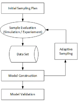
The key stages for constructing a surrogate model includes:

(42)

In this step, we create the initial sampling plan that ensures design space coverage

with limited number of samples.

2. Model Construction:

Using the available samples, we train a mapping function (the surrogate model)

that fits the observed data points well without losing its capability of predicting

unobserved ones.

3. Adaptive Sampling:

This stage identifies the design space regions that has suboptimal predictive

perfor-mance (due to nonlinearity, for instance), and sequentially add additional samples in

those regions.

4. Model validation:

In this steps, we evaluate the final model and validate its quality.

The flowchart is shown in Figure 2.1. We will discuss each of these procedures in detail

in the upcoming sections.

2.2 Sampling Plan

Compared to other supervised learning regression models, surrogate models emphasize on

data efficiency, as the amount of samples is severely limited by the computational expense.

Therefore, it is crucial to have a high-quality initial sampling plan or design of experiment

(43)

Figure 2.1Key surrogate modeling stages

As discussed in the introduction, we would like to define a sampling planX=_{x(1)_,_x(2)_{, ...,}_x(m)_{} ⊂}

D, and execute the expensive simulations/experiments to obtain the corresponding results y=_{y(1)_,_y(2)_{, ...,}_y(m)_}₌_f ₍_X₎_.

Several metrics exists to measure the goodness of a sampling plan. In this section we

will focus on a widely used scalar criterion proposed by Morriset al.[98].

For an existing sampling planXcomprised ofm n-dimensional samples,_{x(i)_}

(44)

we define the pairwise distance between two samples as thel-norm of their difference:

d(x(i),x(j)) =

n

X

d=1

|x_d(i)−x_d(i)|l

1 l

(2.2)

where x_d(i) is the d-th element of the i-the vector in X. Note whenl = 1 we have a

Manhattan distance, and whenl =2 aEuclidean distanceis defined.

Given this definition ofd(x(i),x(j)), we sort the thek= m₂pairwise distances in ascending order to form a distance vector{d1, ...,dk}, where in[98], and many other literatures, these

are named inter-site distances. Then let Ji be the number of sample pairs that can be

separated bydi, we have another vector(J1, ...,Jk)called theindex vector.

The DOEs are thus ranked with the following scalar metric where a lower value ofΦ_q

indicated a better design:

Φq(X) =

k

X

i=1

Jid_i−q

1 q

(2.3)

The issue of choosing an adequateq is still open in this definition. Whenq is large enough, the best plan found using Equation (2.3) will coincide with the well-knowmaximin

criteria proposed by Johnsonet al.[61], but suchΦq’s are difficult to optimize. Instead,q

can be 20 to 100, depending on the complexity of the experiment design problem[33].

With this scalar metric, the pursuit of a high quality DOE is then transferred to an

opti-mization task that can be handled with global optiopti-mization algorithms such as simulated

(45)

2.2.1 Latin Hypercube Sampling

Due to the limitation of computation, it is desirable to have a small sample number while

ensuring uniform coverage of the design space. A brute force way is to construct a full

factorial stratification, but it is too expensive to be feasible, hence fractional stratification

designs are more practical. In this section, we introduce the Latin Hypercube Sampling

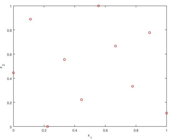
(LHS), a widely used technique for constructing sampling plans.

The primary goal of stratified sampling is to ensure the uniform distribution of

pro-jections on all variable axes[94]. To generate a sample plan with sizem and dimensionn, LHS evenly divides each dimension intom bins, and place samples in the bins such that each occupied bin can escape the design space along any dimension without encountering

other occupied bins.

For illustration, Figure 2.2 shows a 2-D LHS designs on the design space[0, 1]2_{using 10} points.

2.3 Model Construction

Based on the sampling plan introduced in the previous section, we can obtain the

cor-responding evaluations from simulations/experiments. In this part, we will conduct an

overview of the predictive model types used in this dissertation, while the details on each

model type are distributed throughout the following chapters.

Broadly speaking, there are two categories of models:parametricmodels and nonpara-metricmodels[36].

(46)

Figure 2.2A 2-D example of latin hypercube sampling (10 points)

the data under investigation. That is to say, once the parameterw is learned, all future predictions on the input variablex can be made without referring to the training data set

D:P(x|w,D) =P(x|w). Therefore, the complexity of parametric models is bounded by the parameter number, even if the data set is unbounded, but in return, it has a constant time

complexity regardless of how large the training set is.

On the other hand, nonparametric models assume that the intrinsic data distribution

cannot be defined using such a finite parameter set, the "parameter set" should have infinite

dimensions, another way of interpreting it is that it is a set of "functions". Nonparametric

models have better flexibility than parametric ones, but their speed and scalability is harmed

when dealing with big data set.

(47)

that can be extended to various more complicated forms - thelinear regressionmodel, and leave the discussion of nonparametric model including Gaussian processes and Student-t

processes in Chapter 4.

2.3.1 Linear Regression

Suppose the input dimension isn and we havem training samples, given the sample set(X,y) = (x(1)_,_y(1)₎_,₍_x(2)_,_y(2)₎_{, ...,}₍_x(m)_,_y(m)₎

, in whichX_∈R(m×n),x∈Rn,y∈ R(1×n), and y ∈R, our goal is to find a mapping function ˆf :Rd→Rthat represents the input-output

relationships and can be used to predict the results of unseen samples.

As a first step, we consider ˆf to be a linear combination of the inputs:

ˆ

f(x,w) =w0x0+w1x1+w2x2+... (2.4)

where the model parametersw=_{w0,w1,w2, ...}. In particular,w0is called the intercept term andw1,w2, ... are the weights of corresponding input variables (x1,x2, ...). We conven-tionally set a dummy variablex0=1 for the convenience of compact matrix multiplication notation, therefore, Equation (2.4) is rewritten as:

ˆ

f(x,w) =wTx. (2.5)

Intuitively, we can use the differences between model predictions and the true observed

results to quantify the quality of the linear model. Theloss function L(w)is:

L(w) =1 2

m

X

i=1

ˆ

(48)

Note, the coefficient 1₂ at the beginning is used for simplifying notations, as we shall see later. The "learning" process is essentially finding thewwhich minimizesL(w), this is commonly known asleast square estimation.

There are two ways of finding thewthat has the minimum loss: one can either derive thenormal equations, when the closed form equation is available, or use optimization algorithms such as gradient descent. Here we show the former approach.

First, rewrite Equation (2.6) in the matrix form below:

L(w) =1

2(Xw−y)

T₍

Xw₋y). (2.7)

To find the derivatives ofL(w)with respect tow, we have:

5wL(w) =5w

1

2(Xw−y)

T₍

Xw−y)

=1

25w(w

T_XT_Xw

−2yTXw+yTy)

=XTXw−XTy.

(2.8)

The second step holds becauseyT_Xw_{is a scalar.}

As the Hessian₅2

wL(w) =X

T_X_{is positive semi-definite, the}_w_{that minimizes}_L₍_w₎_is

indeed thewthat makes₅_wL(w) =0. Therefore:

w= (XTX)−1XTy. (2.9)

(49)

violated in real applications, and we will further address it in the next part.

2.3.2 Probabilistic View of Linear Regression

In the previous section, we formulated the linear regression problem using least square

approach. We now switch to the probabilistic formulation.

Assume the output is corrupted by random errors that contain random noise or

uncap-tured effects, denoted asε, we can update Equation (2.5) as:

y(i)=wTx(i)+ε(i). (2.10) In canonical statistical learning, aside from the assumption thatyhas linear relationship withx, four more assumptions about{ε(i)_}_{need to be satisfied, namely:}

1. Independence:_{ε(i)_}_{are independent}

2. Homoscedasticity:{ε(i)_}_{have constant variance}

3. Normality:_{ε(i)_}_{are Normally distributed with a zero mean}

It is reasonable to model these errors as identical and independently distributed (i.i.d)

(50)

Therefore:

ε(i)₌₍_y(i)₋_wT

x(i))∼ N(0,σ2) (2.11)

p(y(i)|x(i);w) =_p 1 2πσexp

−(y

(i)₋_wT_x(i)₎2 2σ2

. (2.12)

Here, the notationp(y(i)_|_x(i)_;_w₎_{means the probability is not conditioned on}_{w, as they}

are not random variables.

Equation (2.12) gives the probability thaty(i)_{happens when the the input}_x(i)_{is given to}

the model which is parameterized byw, this is the same as the probability that the model correctly predicts the result ofx(i). As the error termsε’s are i.i.d. distributed, the overall probability of a correct model is the probability product:

L(w) =

m

Y

i=1

(p(y(i)|x(i);w))

=

m

Y

i=1

1 p

2πσexp

−(y

(i)₋_wT_x(i)₎2 2σ2

(2.13)

Equation (2.13)is commonly known as thelikelihoodof the model, and the principle of

maximum likelihoodgives a way of choosing the best model by maximizing it. However, in practice, maximizing (2.13) directly will complicate derivation and give rise to arithmetic

underflow in floating number calculation, we instead use the strictly increasing natural

(51)

l(w) =logL(w)

=log

m

Y

i=1

1 p

2πσexp

−(y

(i)₋_wT_x(i)₎2 2σ2

=

m

X

i=1

log_p 1 2πσexp

−(y

(i)₋_wT_x(i)₎2 2σ2

=mlog_p1 2πσ−

1 2σ2

m

X

i=1

(y(i)−wTx(i))2

(2.14)

Apparently, maximizing (2.14) is equivalent to minimizing 1₂Pm_i₌₁(y(i)₋_wT_x(i)₎2_{, and} hence corresponds to the least-square loss function defined in (2.9). Thewobtained through maximizingl(w)is called themaximum likelihood estimate (MLE):

wM L E = (XTX)−1XTy (2.15)

Theoretically, the MLE estimate minimizes the Kullback-Leibler divergence (KL

diver-gence), which can be thought as the "distance" from the (true) underlying distribution to

the model distribution. The proof is beyond the scope of this dissertation and we direct the

interested readers to[10]for a thorough treatment.

2.3.3 Nonlinear Features and Basis Functions

In the previous section, we have discussed how to use linear regression to construct a

predictor based on the existing data. One of the biggest limitation of the simple linear

regression model is that it assumes the output to be a linear combination of the inputs,

(52)

section, we will start with polynomial linear regression models to discuss the methods for

handling nonlinearity with polynomial basis functions and then introduce the commonly

used radial basis function (RBF) kernel.

2.3.3.1 Polynomial Regression Model

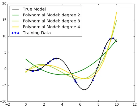
In Figure 2.3, we show the limitation of using simple linear regression model when

deal-ing with nonlinearity. A natural extension to linear regression model is to use nonlinear

combinations of the features. For instance, for a single variable (e.g. x), we can include higher-order terms such asx2_,_x3_,_etc._{to introduce "more" features into the linear model.} Figure 2.4 demonstrates the improved results by incorporating 2nd and 3rd order terms,

respectively.

Including higher order terms in the inputs is known asfeature mapping, by which the original (n-dimensional) inputs are mapped to a new (k-dimensional)feature space

with the mapping functionφ(x):_Rn_→

Rk, this mapping function is also called thebasis function. For instance, we can express the 3rd order case as:

φ(x) =

     x x2 x3      (2.16)

Exchanging thexin basic linear regression with the basis functionφ(x), the polynomial regression is then:

ˆ

(53)

Figure 2.3Handling nonlinear data with Linear Regression, created with the scikit-learn package [109]

If we let

Φ=



      

−φ1(x)− −φ2(x)−

...

−φk(x)−



      

(2.18)

Following the same procedure of deriving the normal equation, one can also obtain the

least-square solution for weightswwith respect to the basis function:

(54)

Figure 2.4Handling nonlinear data with Polynomial Regression, created with scikit-learn pack-age

This is indeed the result of substituting theXin Equation (2.9)/(2.15) withΦ.

2.3.3.2 Radial Basis Functions

There are many other basis functions besides polynomial , we will follow on by introducing

one of the most popular one called theradial basis functions. The radial basis function takes the following form:

φ(x) =exp

−(x−c) 2 σ2

(2.20)

(55)

while vanishes whenxmoves away from the center. The parameterσcontrols the decay rate ofφ(x)asxmoves away: a smallerσwill cause a faster decay.

Suppose we havek centers, the feature space is hencek-dimensional, and the approxi-mation function is:

ˆ

f(x,w) =wTφ(x) =

k

X

i=1

exp

−(x−c

(i)₎2 σ2

wi (2.21)

One can interpret this as a weighted sum of "bell-shaped" curves centered atcwhich can be randomly picked or simple use each sample as a center, but this will potentially

introduce the risk of overfitting. Besidesw, RBF regression adds one more parameterσ, a standard approach for picking the value ofσis through cross validation. Both overfitting

and cross validation will be covered later in this chapter.

The RBF model demonstration for the same 1-D dataset is shown in Figure 2.5.

2.3.4 Regularization

Recall that we mentioned the potential problem with the normal equation (2.9) in the linear

regression section, where(XTX)−1may not exist due to the poorly conditioned(XTX)matrix. For example, whenm=20 andn=2000,(XT_X₎_{will seldom be full-rank, and thus invertible.}

One way to handle this singular matrix issue is through adding small elements along the

matrix diagonal to "stabilize" it.

Another way to look at regularization is that it is trying to suppress the model

IC Design Analysis, Optimization and Reuse via Machine Learning.

ABSTRACT

DEDICATION

BIOGRAPHY

ACKNOWLEDGEMENTS

CONTENTS

LIST OF TABLES

LIST OF FIGURES

CHAPTER

1

INTRODUCTION

1.1

Motivation

1.2

Related Works I: Analog Optimization and IP Reuse

1.2.1

Knowledge-based approaches

1.2.2

Optimization-based approaches

1.2.3

Analog Optimization and IP Reuse Summary

1.3

Related Works II: Yield Estimation

1.3.1

Crude Monte Carlo

1.3.2

Efficient Monte Carlo techniques

1.3.3

Yield Analysis Summary

1.4

Disseration Organization

1.5

Research Contributions

CHAPTER

2

SURROGATE MODEL FUNDAMENTALS

2.1

Introduction to Surrogate Modeling

2.2

Sampling Plan

2.2.1

Latin Hypercube Sampling

2.3

Model Construction

2.3.1

Linear Regression

2.3.2

Probabilistic View of Linear Regression

2.3.3

Nonlinear Features and Basis Functions

2.3.4

Regularization