Backscattering Analysis for Snow Remote Sensing Model
with Higher Order of Surface-Volume Scattering
Syabeela Syahali1, * and Hong Tat Ewe2
Abstract—The study of earth terrain in Antarctica is important as this region has a direct impact on global environment and weather condition. There have been many research works in developing remote sensing technologies, as it can be used as an earth observation technique to monitor the polar region [11, 15]. In previous studies, remote sensing forward model has been developed to study and understand scattering mechanisms and sensitivity of physical parameters of snow and sea ice. This paper is an extended work from previous studies [16–19], where an improved theoretical model to study polar region was developed. Multiple-surface scattering, based on an existing integral equation model (IEM) that calculates surface scattering and additional second-order surface-volume scattering, were added in the model from prior research works [7] for improvement in the backscattering calculation. We present herein the application of this model on a snow layer above ground which is modeled as a volume of ice particles that are closely packed and bounded by irregular boundaries above a homogenous half space. The effect of including multiple surface scattering and additional surface-volume scattering up to second order in the backscattering coefficient calculation of snow layer is studied for co-polarized and cross-polarized returns. Comparisons with satellite data are also done for validation. Results show improvement in the total backscattering coefficient for cross-polarized return in the studied range, suggesting that multiple-surface scattering and surface-volume scattering up to second order are important scattering mechanisms in the snow layer and should not be ignored in polar research.
1. INTRODUCTION
In Antarctica, most parts of the continent are covered by layer of snow, and it is common to find snow layer on top of the sea ice. Understanding the interaction and scattering mechanisms between electromagnetic waves and snow is important to have improved interpretation of satellite images. This can be achieved by developing a reliable forward model where given physical configuration of snow layer characterized by a number of physical parameters, the model can be used to study the interaction of incoming microwave and the snow medium and calculate the backscattering of microwave from the medium to be received by remote sensing satellites. A remote sensing forward model is also useful in the development of an inverse model that allows retrieval of physical parameters of the medium from the measured satellite radar returns using microwave remote sensing [13], since it is also an important tool in studying the sensitivity of physical parameters in this area.
Snow area can be modelled as an electrically dense medium bounded on the top and bottom by irregular boundaries. A medium is considered electrically dense if the average separation between the scatterers (in this case ice particles in the background medium of air) is less than a wavelength of incoming microwave. In this layer bounded by top and bottom rough surfaces, in addition to the common direct surface scattering, volume scattering and first order surface-volume scattering, multiple surface scattering and second order surface-volume scattering may occur and contribute towards the
Received 26 December 2015, Accepted 9 April 2016, Scheduled 19 April 2016 * Corresponding author: Syabeela Syahali ([email protected]).
total backscattering coefficient. Incident waves on a surface are scattered and may be rescattered back to incident direction if the surface is rough. Incident wave may also be scattered twice by scatterers, in the surface-volume scattering process, when the medium is electrically dense.
It is essential to develop a reliable theoretical model to study the medium where multiple surface scattering and second order surface-volume scattering may be important, to better understand these effects. In a previous work [7], a backscattering model for an electrically dense medium was developed. It was modeled as a layer of a discrete inhomogeneous medium, where randomly distributed ice spherical scatterers are embedded in homogeneous medium in the layer. This layer is bounded on the top and bottom by irregular surface boundaries. Above the layer is air, and below the layer can be a homogenous half space where this can be used to represent earth ground layer beneath the snow or a very thick layer of sea ice beneath the snow layer with high attenuation rate of wave penetration. For ice shelf, this can be a very thick layer of compacted snow on top of the ocean. The spherical scatterer is modelled as a Mie scatterer characterized by Mie scattering. This medium is considered electrically dense where the spacing between the scatterers is comparable to the wavelength [6]. The modified phase matrix for Mie scatterers based on the dense medium phase and amplitude correction theory (DM-PACT) [4] were taken into account to consider the close spacing effects of the scatterers. Radiative transfer theory [3] was used to calculate the backscattering coefficient of this medium. The radiative transfer equation was solved iteratively up to the second order. Three major scattering mechanisms were derived based on [9], which are direct surface scattering, surface-volume scattering and volume scattering. IEM was used to calculate the top and bottom rough surfaces. However, the IEM used in [7] accounts for single scattering only, and this requires further improvement by also considering multiple surface scattering.
In this study, improvement is done in the surface scattering formulation by including the surface multiple scattering terms. Currently, many versions of IEM model for single and multiple surface scattering are available [2, 10, 21, 22]. In this study, we use the original IEM with both single and multiple scattering to model the top and bottom surfaces. The formulation of the surface scattering model is obtained from [9]. Improvement is also done in the surface-volume scattering formulation where additional surface-volume scattering terms up to second order are derived and also included in the model. The effect of including these terms in the backscattering coefficient calculation for total and each scattering mechanism is studied. Results from theoretical analysis experiment show improvement in the total backscattering coefficient mostly for cross-polarized return. Promising match is also observed from the results of comparing the developed model with satellite data.
2. MODEL FORMULATION
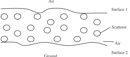
The cross section of the dense medium for snow layer used in the theoretical modeling is shown in Figure 1. The layer is modeled as a volume of randomly distributed ice particles as the Mie scatterers that are closely packed and bounded by irregular boundaries. Parameters such as radius, permittivity and volume fraction are used to configure these scatterers. The ground is treated as homogenous half space. The air-snow boundary and snow-ground boundary are labelled as surface 1 and surface 2 in Figure 1. Surface 1 and surface 2 are rough surfaces with parameters of surface root mean square (rms) height and correlation length. The surfaces are characterized by the roughness spectrum of the exponential correlation function, based on the correlation length and rms height of the surface. In electrically dense medium where there is more than one scatterer within the distance of a wavelength, the spatial arrangement of the scatterers has been shown to significantly affect its scattering properties [4, 5, 12, 20]. These effects are taken into account by applying the Dense Medium Phase and Amplitude Correction Theory (DM-PACT) [4, 5] for the phase matrix of the Mie scatterer. DM-PACT includes two types of correction which are phase correction and amplitude correction in the phase matrix. This is based on the concept of antenna array where instead of treating the scatterrers as independent scatterrers, the relative phase contributions of them are added up and included in the volume phase matrix.
The Radiative Transfer Equation [3] characterizes the propagation and scattering of specific intensity inside a medium and is given by
cosθdI¯
dz =−¯¯κeI¯+
∫
¯ ¯
Scatterer
Air
Surface 2 Surface 1
Ground
Figure 1. Cross section of snow layer.
where ¯I is the Stokes vector, ¯κ¯e the extinction matrix, and ¯P¯ the phase matrix of the medium. The
phase matrix ¯P¯ is given as ¯ ¯
P(θ, ϕ;θ′, ϕ′) =⟨|ψ|2⟩n·S¯¯= [
Pvv Pvh
Phv Phh ]
(2)
where ⟨|ψ|2⟩n is the dense medium phase correction factor [4], and ¯S¯ the Stokes’ matrix with close
spacing amplitude correction [8], and theta, phi, theta′ and phi′ are scattered and incident elevation and azimuth angles. Stokes’ matrix relates the scattered intensities to the incident intensities on a Mie scatterer. The Stokes’ matrix of the single scatterer is multiplied by a dense medium phase correction factor to get the phase matrix for a collection of scatterers. The close spacing amplitude correction appears inside the Stokes matrix, where the near-field terms of the scattered fields of a Mie scatterrer are included in it.
In [7] and [9], this radiative transfer equation was solved iteratively up to second order solutions. Zeroth order solutions characterize the scattering process without any scatterer involved whereas first and second order solutions characterize the scattering process involving one and two scatterers, respectively. Through this iterative solutions, many scattering terms were derived and calculated.
To understand the various scattering mechanisms involved in this, the solutions were grouped into three major scattering terms which contributes to the overall backscattering return. These are the surface scattering terms, surface-volume scattering terms and volume scattering terms. The upward scattered intensityI is related with the backscattering coefficient, σ, by this formula;
σpq =
4πcosθsT01I1+pq
Ii
(3)
2.1. Surface Scattering
The surface scattering term is the zeroth order solution of Equation (1) and is given by
σpqs =σspq1+σspq2 (4) whereσs1
pq andσspq2 are given by
σspq1(θs, ϕs;θi, ϕi) =σpqo1(θs, ϕs;θi, ϕi) (5)
and
σpqs2(θs, ϕs;θi, ϕi) = cosθsT1tp(θs, θts)Tt1q(θti, θi) secθtsLp(θts)Lq(θti)σpqo2(θts, ϕts;θti, ϕti) (6)
σpqs1andσspq2 are the scattering terms from the top and bottom surfaces, respectively. σpqo1 andσpqo2are the bistatic scattering coefficients of the top and bottom surfaces based on the IEM rough surface model.
θsandθi are the scattered and incident angles in the air, whileθts andθtiare the scattered and incident
angles in the layer. T10 and T01 are the transmissivity from the top boundary into the layer, and from
the layer into the top boundary, respectively, andLu is the attenuation of intensity through the layer.
The IEM rough surface model used in this study accounts for both single and multiple scattering. The formulation is obtained from [9] and given by
The first term is the Kirchhoff term and accounts for single scattering only. It is given by:
σqpk(s) = 0.5k2|fqp|2exp [
−σ2(ksz+kz)2 ]∑∞
n=1 [
σ2(kkz+kz)2 ]n
W(n)(ksx−kx, ksy−ky)
n! , (8)
where kx = ksinθcosϕ, ky = ksinθsinϕ, kz = kcosϕ, ksx = ksinθscosϕs, ksy = ksinθssinϕs,
ksz = kcosϕs, k is the incident wavenumber, σ2 the variance of the surface, fqp the tangential field
coefficient andW(n) thenth power roughness spectrum.
The second term is the cross term. The single-sum terms are single scattering terms, and the double-sum term represents multiple scattering; it is given by
σqpkc(s) = 0.5k2exp[−σ2(ksz2 +k2z+kzksz) ]
Re
{
fqp∗ [
Fqp(−kx,−ky) ∞ ∑
n=1 [
σ2ksz(kz+ksz) ]n
n! W
(n)(k
sx−kx, ksy−ky)
+Fqp(−ksx,−ksy) ∞ ∑
m=1 [
σ2kz(kz+ksz) ]m
m! W
(m)(k
x−ksx, ky −ksy)
+ 1 2π ∞ ∑ n=1 [
σ2ksz(kz+ksz) ]
n!
n∑∞
m=1 [
σ2kz(kz+ksz) ]m
m!
∫∫
Fqp(u, v)Wn(ksx+u, ksy+v)Wm(kx+u, ky+v)dudv ]}
(9)
where Fqp is the complementary field coefficient. Finally, the third term is the complementary term.
The single-scattering terms are the terms with one sum, and multiple scattering is represented by terms with more than one sum and given below:
σqpc (s) = 0.125k2exp[−σ2(k2sz+kz2)]·
{
|Fqp(−kx,−ky)|2 ∞ ∑
m=1
(σ2k2sz)m
m! W
(m)(k
sx−kx, ksy−ky)
+Fqp(−kx,−ky)Fqp∗(−ksx,−ksy) ∞ ∑
n=1
(σ2kzksz)n
n! W
(n)(k
sx−kx, ksy−ky)
+Fqp∗(−kx,−ky)Fqp(−ksx,−ksy) ∞ ∑
m=1
(σ2kzksz)m
m! W
(m)(k
sx−kx, ksy−ky)
+|Fqp(−ksx,−ksy)|2 ∞ ∑
n=1
(σ2k2z)n
n! W
(n)(k
sx−kx, ksy−ky) +
1 2π
∞ ∑
m=1
(σ2k2sz)m
m!
∞ ∑
n=1
(σ2k2z)i
i! ·
∫∫
|Fqp(u, v)|2W(m)(ksx+u, ksy+v)W(i)(kx+u, ky+v)dudv
+ 1 2π ∞ ∑ n=1 ∞ ∑ m=1
(σ2kzksz)n+m
n!m! ·
∫∫
Fqp(u, v)Fqp∗ [−(u+kx+ksx),−(v+ky+ksy)]
·W(n)(ksx+u, ksy+v)W(m)(kx+u, ky+v)dudv} (10)
2.2. Surface-Volume Scattering
After solving Equation (1) iteratively, the first order solution is given by:
Il+(0, θ, ϕ) =R12(θ, π−θ)S−(−d, π−θ,ϕ)e−K +
e secθ(d)+S+(0, θ, ϕ) (11)
where I+ is the upward intensity, R the reflectivity matrix, d the depth of the layer, Ke the volume
Layer
1 Layer 2
Figure 2. Scattering mechanisms from the first term of Equation (11).
1
Layer
2
Figure 3. Scattering mechanisms from the second term of Equation (11).
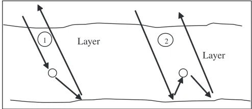
The first term describes the downward scattered intensity from the first scatterer being reflected into upward scattered intensity by the lower boundary, while the second term describes the upward scattered intensity from the first scatterer. The scattering mechanisms which can be derived from the first and second terms are illustrated in Figures 2 and 3, respectively. These terms yield the first-order surface-volume scattering components, which are grouped into the following terms [7];
σpqvs =σpqvs(m→s2) +σpqvs(s2→m) (12) and also the first-order volume scattering component, which will be described in Section 2.3. σpqvs(m→ s2) andσvspq(s2→m) are volume to surface and surface to volume interaction terms, illustrated as term 1 of Figure 2 and term 2 of Figure 3, respectively. The surface considered in surface-volume scattering process is the bottom surface. In this study, more surface-volume scattering terms up to the second order are included in the formulation. The first term added, which is of first order, is the surface to volume to surface interaction term illustrated by term 2 of Figure 2 and given by:
σ1pq(θs, ϕs, π−θi,ϕi) =
cosθs
4π T01(θs,θ1s)T10(π−θ1i,π−θi)L
−
q(θ1i)Lp+(θ1s) secθ1s 2π
∫
0 π 2 ∫
0 2π ∫
0 π 2 ∫
0
secθ′′sinθ′′dθ′′dϕ′′secθ′sinθ′dθ′dϕ′
∑
t=v,h ∑
..u=v,h
Ptu(π−θ′′, ϕ′′, θ′, ϕ′)σuq(θ′, ϕ′, π−θ1i,ϕ1i)σpt(θ1s, ϕ1s, π−θ′′, ϕ′′) [
1−L+u(θ′)L−t (θ′′) (Keu+ secθ′+Ket−secθ′′)
]
(13)
Layer
1 5
6 2 Layer
Layer
Layer Layer
Layer 3
4
Figure 4. Scattering mechanisms from the first term of Equation (14).
7 11
12
8 Layer
Layer
Layer
Layer Layer
Layer 9
10
Figure 5. Scattering mechanisms from the second term of Equation (14).
Next, second-order iterative solutions of the radiative transfer equation, which represent surface-volume scattering as mentioned above, are given by:
I2+(0, θ, ϕ) =R12(θ, π−θc)S1−(−d, π−θc, ϕc)e−K +
e secθ(d)+S+
1(0, θ, ϕ) (14)
are considered not important to be included. Term 1 is given by:
σ2pq(θs, ϕs, π−θi,ϕi) = cosθssecθ1sT01(θs,θ1s)T10(π−θ1i, π−θi) ∫ 2π
0 ∫ π
2
0
secθ′sinθ′dθ′dϕ′
2π ∫ 0 π 2 ∫ 0
secθcsinθcdθcdϕc ∑
t=v,h ∑
.u=v,h
(P2tu(π−θc, ϕc, π−θ′, ϕ′)Puq(π−θ′, ϕ′, π−θ1i, ϕ1i)
σpt(θ1s, ϕ1s, π−θc, ϕc)L+p(θ1s)L (15)
and term 3 is given by:
σ2pq(θs, ϕs, π−θi,ϕi) = cosθssecθ1sT10(π−θ1i, π−θi)T01(θs,θ1s) ∫ 2π
0 ∫ π
2
0
secθ′sinθ′dθ′dϕ′
2π ∫ 0 π 2 ∫ 0
secθcsinθcdθcdϕc ∑
t=v,h ∑
.u=v,h
P2tu(π−θc, ϕc, θ′, ϕ′)Puq(θ′, ϕ′, π−θ1i, ϕ1i)
σpt(θ1s, ϕ1s, π−θc, ϕc)L+p(θ1s)L (16)
The second term of Equation (14) describes the upward scattered intensity from the second scatterer. All the scattering mechanisms which can be derived from this first term are illustrated as terms 7 to 12 in Figure 5. Terms 7 and 9 are the terms for second-order volume scattering which will be described in Section 2.3. Term 12 is ignored due to high loss. Terms 8, 10 and 11 are derived in this study and given below respectively:
σ2pq(θs, ϕs, π−θi,ϕi) = cosθssecθ1sT10(π−θ1i, π−θi)T01(θs, θ1s) secθ′′ 2π ∫ 0 π 2 ∫ 0
secθ′sinθ′dθ′dϕ′
2π ∫ 0 π 2 ∫ 0
secθ′′sinθ′′dθ′′dϕ′′ ∑
t=v,h ∑
.u=v,h
P2pt(θ1s, ϕ1s, π−θ′, ϕ′)
Ptu(π−θ′, ϕ′, θ′′, ϕ′′)σuq(θ′′, ϕ′′, π−θ1i, ϕ1i)L−q(θ1i)L (17)
σ2pq(θs, ϕs, π−θi,ϕi) = cosθssecθ1sT10(π−θ1i, π−θi)T01(θs,θ1s) secθ′′ 2π ∫ 0 π 2 ∫ 0
secθ′′sinθ′′dθ′′dϕ′′
2π ∫ 0 π 2 ∫ 0
secθ′sinθ′dθ′dϕ′ ∑
t=v,h ∑
.u=v,h
P2pt(θ1s, ϕ1s, θ′, ϕ′)Ptu(θ′, ϕ′, θ′′, ϕ′′)
and
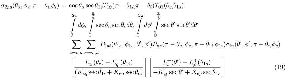
σ2pq(θs, ϕs, π−θi,ϕi) = cosθssecθ1sT10(π−θ1i,π−θi)T01(θs,θ1s) 2π
∫
0
dϕc π 2 ∫
0
secθcsinθcdθc 2π ∫
0
dϕ′
π 2 ∫
0
secθ′sinθ′dθ′
∑
t=v,h ∑
.u=v,h
P2pt(θ1s, ϕ1s, θ′, ϕ′)Puq(π−θc, ϕc, π−θ1i,ϕ1i)σtu(θ′, ϕ′, π−θc,ϕc) [
L−u(θc)−L−q(θ1i)
(Keq−secθ1i+Keu− secθc) ] [
L+t (θ′)−L+ p(θ1s)
−Ket+secθ′+Kep+secθ1s ]
(19)
2.3. Volume Scattering
The volume scattering term from the first- and second-order solution of Equation (1) can be regrouped based on different scattering processes of the scatterers and are shown as
σpqv =σvpq(up, down) +σpqv (up, down, down) +σpqv (up, up, down) (20) and illustrated in term 1 of Figure 3 and terms 7 and 9 in Figure 5, respectively. The first term describes the intensity being scattered by one scatterer, while the second and third terms describe the intensity being scattered by two scatterers. The arguments in the terms describe the upward and downward directions of the intensity throughout the scattering process, starting from the right to left.
3. RESULT AND DISCUSSION
3.1. Theoretical Analysis
The developed model is applied to the snow layer. The parameters are obtained from [7] and shown in Table 1. Backscattering coefficient is calculated for frequency 5 GHz, over an incident angle range from 10◦ to 60◦. The effect of including multiple surface scattering and additional surface-volume scattering up to second order in the backscattering calculation of snow layer is analysed for the co-polarized and cross-polarized return. Results from [7] are included in the figure for comparison. For the ease of reference, the model developed in this paper is referred to as Multiple Surface and Surface-Volume of 2nd Order (MSSV2) model.
Table 1. Model parameters for theoretical analysis.
Parameters Estimated Values
Frequency/GHz 5
Scatterer Radius/mm 0.5
Volume fraction/% 30
Effective relative permittivity of top layer (1.0, 0.0) Relative permittivity of sphere (3.15, 0.015) Background relative permittivity (1.0, 0.0)
Lower half-space permittivity (5.0, 0.0)
Thickness of layer/m 0.5
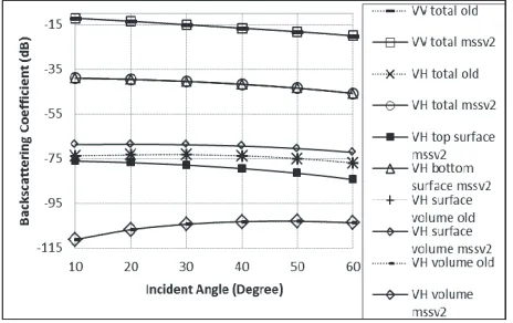
Figure 6 shows the total and each component of backscattering coefficient. For theV V polarized return, no improvement is seen as expected, because in co-polarized surface backscattering, single surface scattering is dominant instead of multiple surface scattering. Contribution from surface-volume scattering is also very small. On the other hand, significant improvement is seen for cross-polarized backscattering return as the effect of including multiple surface scattering and additional surface-volume scattering up to the second order. By studying each component, it can be seen that the current model with MSSV2 is able to calculate the cross-polarized surface scattering contribution since cross-polarized surface backscattering return results only from multiple surface scattering. Bottom surface scattering is dominating, indicating multiple surface scattering on the snow-ground interface is important. Significant improvement is seen in surface-volume scattering, indicating the presence of second-order surface-volume scattering in the snow layer. Surface-volume scattering is the next important scattering after bottom surface scattering. Therefore, the improvement seen in the total backscattering coefficient is due to multiple surface scattering on the bottom surface and second-order surface-volume scattering.
To study the effect for higher frequency, incident angle is fixed at 15 degrees, and backscattering return for total and each component of scattering for cross-polarization over frequency is plotted for frequency 5 GHz to 35 GHz in Figure 7. Further increase in frequency shows that bottom surface scattering contribution continues to drop. As snow becomes more lossy and electrically denser with increasing frequency, less energy is scattered directly from the bottom surface due to higher attenuation in the medium. Contribution from surface-volume scattering continues to increase until frequency is over 30 GHz. There is a significant difference between the two models for the total backscattering coefficient, until frequency is about 30 GHz. This difference is due to multiple scattering at the bottom surface at lower frequency and surface-volume scattering up to second order at higher frequency. At very high frequency, when volume scattering starts dominating, multiple scattering and surface-volume scattering up to second order are no longer important.
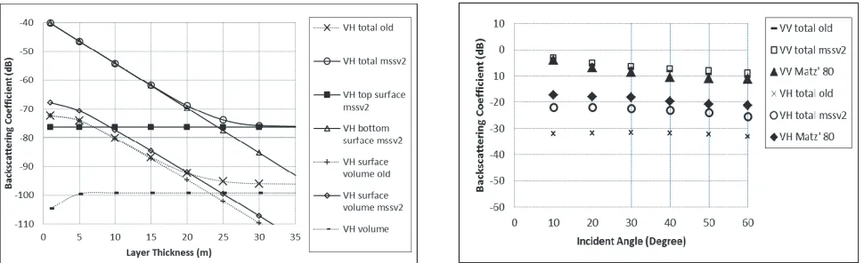
To study the effect of higher layer thickness, incident angle and frequency are fixed at 15 degrees 5 GHz, and V H backscattering return for total and each component of scattering over different layer thicknesses is plotted for layer thickness from 1 m to 35 m in Figure 8. For total backscattering return, there is significant change between the previous model and MSSV2 for all the layer thickness. For small thickness, the improvement in total backscattering is due to multiple scattering on the top and bottom surfaces and surface-volume scattering. It can be seen that contribution from the bottom surface and surface-volume scattering decreases as thickness increases, when less signal reaches the bottom surface. Volume scattering increases because of more scattering activity in the snow layer. After 5 m, the contribution from volume scattering becomes constant. The total scattering decreases as thickness increases, until about 30 m of layer thickness, after which it becomes constant due to multiple scattering on top surface alone.
Theoretical analysis shows that only MSSV2 gives return for cross-polarized surface scattering, since contribution from cross-polarized surface backscattering is only from the surface multiple scattering
Figure 6. Backscattering coefficient against incident angle.
Figure 8. Backscattering coefficient against layer thickness at 5 GHz frequency and 15◦ incident angle (V H polarized).
Figure 9. Backscattering coefficient of model prediction and measurements by Matzler et al..
process. Surface multiple scattering and surface-volume scattering up to the second order are very important in cross-polarized backscattering, when there is contribution from surface scattering and surface-volume scattering. However, as can be seen in Figures 7 and 8, as volume scattering increases, the improvement in total backscattering decreases. As expected, this MSSV2 model does not give any improvement to the total backscattering coefficient when the scattering mechanism is dominated by volume scattering. This shows that although this model gives significant improvement in snow area for cross-polarized scattering, higher order volume scattering may be added to improve the scattering for snow area with significant volume scattering contribution. For co-polarized backscattering, surface multiple scattering and surface-volume scattering up to second order are not important in the range studied.
3.2. Comparison with Measurement Results
This model is then compared with data from the ground truth measurement done on dry snow field by [14]. The input parameters used in the model are shown in Table 2 [9, 14]). Those measured parameter used by [14] are incorporated and other parameters are estimated based on [9] and normal range of values for physical parameter of snow layer on ground. Figure 9 shows the V V and V H
polarized returns of the previous model, MSSV2, and measurements by [14]. For V V return, it can
Table 2. Snow parameters used for data from Matzler et al.
Parameters Values Used
Frequency/GHz 10.4
Scatterer Radius/mm 0.78
Volume fraction/% 24
Effective relative permittivity of top layer (1.0, 0.0) Relative permittivity of sphere (3.2, −0.001) Background relative permittivity (1.0, 0.0)
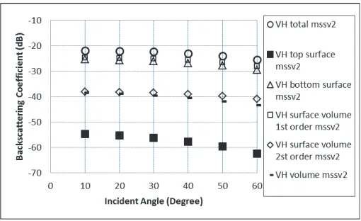
Figure 10. Backscattering coefficient of model prediction (MSSV2) in Figure 9 (V H polarized).
be seen that there is a good match between the model prediction and the measured data. For V H
return, there is significant improvement in the MSSV2. The match between MSSV2 and measurements is generally good, although it is not as good as for co-polarized return. By analysing each scattering component plotted in Figure 10, it is found that volume scattering is significant in this area. Including higher order terms for volume scattering calculation in the model may improve the model prediction.
Comparison with measurement results shows that the backscattering coefficient from MSSV2 gives good match with the measured backscattering coefficient for co-polarized return. The model also gives promising match for cross-polarized return, when surface-volume and volume scattering of higher order are not important scattering mechanisms. Compared with the previous model prediction, there is significant improvement in MSSV2 in cross-polarized scattering, indicating the importance of including surface multiple scattering and surface-volume scattering up to second order. However, this model can be further improved by including higher order solution to its iterative solution.
4. CONCLUSION
In this paper, an improved theoretical model to study snow area is presented. This model takes into account the surface multiple scattering and also the surface-volume scattering which are derived up to the second order. Experiment results from theoretical analysis show that bottom surface scattering and surface-volume scattering for cross-polarized return are important scattering mechanisms in snow area. Hence, it can be concluded that by including the surface multiple scattering terms and the additional surface-volume scattering terms in the theoretical modelling, the total backscattering coefficient in snow area can be improved for cross-polarized return. By comparing this model with the measurements by [14] for validation, promising match is observed. In future, this model can be further improved by considering higher order scattering in the surface-volume formulation, considering the advanced IEM (AIEM) [21] in the surface scattering formulation, and considering multilayer in the model development [1].
ACKNOWLEDGMENT
The authors are thankful for the financial support from the Asian Office of Aerospace R&D (AOARD) [Grant Number: FA2386-12-1-4082/FA2386-13-1-4140], Ministry of Science, Technology and Innovation Malaysia (MOSTI Flagship Grant Number: FP1213E037).
REFERENCES
2. Alvarez-Perez, J., “An extension of the IEM/IEMM surface scattering model,” Waves Random Media, Vol. 11, No. 3, 307–329, 2001.
3. Chandrasekhar, S.,Radiative Transfer, Dover, New York, 1960.
4. Chuah, H. T., S. Tjuatja, A. K. Fung, and J. W. Bredow, “The volume scattering coefficient of a dense discrete random medium,”IEEE Transaction of Geoscience Remote Sensing, Vol. 34, No. 4, 1137–1143, 1996.
5. Chuah, H. T., S. Tjuatja, A. K. Fung, and J. W. Bredow, “Radar backscatter from dense discrete random medium,”IEEE Transaction of Geoscience Remote Sensing, Vol. 35, No. 4, 892–899, 1997. 6. Ewe, H. T. and H. T. Chuah, “A study of dense medium effect using a simple backscattering model,” Proceedings of IEEE International Geoscience and Remote Sensing Symposium, Vol. 3, 1427–1429, 1997.
7. Ewe, H. T., H. T. Chuah, and A. K. Fung, “A backscatter model for a dense discrete medium: Analysis and numerical results,”Remote Sensing of Environment, Vol. 65, No. 2, 195–203, 1998. 8. Fung, A. K. and H. J. Eom, “A study of backscattering and emission from closely packed
inhomogeneous media,” IEEE Transactions on Geosciences Remote Sensing GE, Vol. 23, No. 5, 761–767, 1985.
9. Fung, A. K., Microwave Scattering and Emission Models and Their Applications, 164–275, Artech House, Norwood, MA, 1994.
10. Fung, A. K., W. Y. Liu, K. S. Chen, and M. K. Tsay, “An improved IEM model for bistatic scattering,”Journal of Electromagnetic Waves and Applications, Vol. 16, No. 5, 689–702, 2002. 11. Giles, A. B., R. A. Massom, and R. C. Warner, “A method for sub-pixel scale feature-tracking
using Radarsat images applied to the Mertz Glacier Tougue, East Antarctica,”Remote Sensing of Environment, Vol. 113, No. 8, 1691–1699, 2009.
12. Ishimaru, A. and Y. Kuga, “Attenuation constant of a coherent field in a dense distribution of particles,”Journal of Optical Society of America, Vol. 72, No. 10, 1317–1320, 1982.
13. Lee, Y. J., W. K. Lim, and H. T. Ewe, “A study of an inversion model for sea ice thickness retrieval in Ross Island, Antarctica,” Progress In Electromagnetics Research, Vol. 111, 381–406, 2011. 14. Matzler, C., E. Schanda, R. Hofer, and W. Good,Microwave Signatures of the Natural Snow Cover
at Weissfluhjoch, Vol. 2153, 203–223, NASA Conference Publication, 1980.
15. Park, H., H. Yabuki, and T. Ohata, “Analysis of satellite and model datasets for variability and trends in Arctic snow extent and depth, 1948–2006,” Polar Science, Vol. 6, No. 1, 23–37, 2012. 16. Syahali, S., H. T. Ewe, and S. A. Ibrahim, “Theoretical modeling and analysis of multiple surface
scattering and surface-volume scattering in snow layer,” AKEPTs 1st Annual Young Researchers
Conference and Exhibition (AYRC X3 2011), Kuala Lumpur, December 2011.
17. Syahali, S.,A Study of Surface and Surface-volume Scattering, Lap Lambert Academic Publishing, Germany, 2012.
18. Syahali, S. and H. T. Ewe, “Model development and analysis of multiple surface scattering and surface-volume scattering in sea ice layer,” IEEE Asia-Pacific Conference on Applied Electromagnetics (APACE 2012), Melaka, Malaysia, December 2012.
19. Syahali, S. and H. T. Ewe, “Remote sensing backscattering model for sea ice: Theoretical modelling and analysis,”Advances in Polar Science, Vol. 24, No. 4, 258–264, 2013.
20. Wen, B., L. Tsang, D. P. Winebrenner, and A. Ishimaru, “Dense medium radiative transfer theory: Comparison with experiment and application to microwave remote sensing and polarimetry,”IEEE Transactions on Geoscience and Remote Sensing, Vol. 28, No. 1, 46–59, 1990.
21. Wu, T. D. and K. S. Chen, “A reappraisal of the validity of the IEM model for backscattering from rough surfaces,”IEEE Transactions on Geoscience and Remote Sensing, Vol. 42, No. 4, 743–753, 2004.