Design and Stability Analysis of an Integrated Controller for Highly Flexible Advanced Aircraft Utilizing the Novel Nonlinear Dynamic Inversion

Design and Stability Analysis of an Integrated Controller

for Highly Flexible Advanced Aircraft Utilizing

the Novel Nonlinear Dynamic Inversion.

Thesis by Irene M. Gregory

In Partial Fulfillment of the Requirements for the Degree of

Doctor of Philosophy

California Institute of Technology Pasadena, California

2005

© 2005

v

To my family

I wouldn’t be where I am without you.

Grandpa,

vii

Acknowledgements

This is one section that in a course of writing the dissertation is typically relegated to be the last written and least thought out. I’m sure given some passage of time and reacquired perspective, I will find regrettable omissions both of the people and subjects, and for that I beg forgiveness and understanding.

First and foremost, I would like to thank my advisor, John Doyle, for affording me an opportunity to learn in an exciting and challenging environment and for taking a chance and letting me do a Ph.D. while working full time across the country. John taught me many lessons and exposed me to new experiences and ideas, and for that I will forever be grateful. I want to thank Richard Murray for his guidance through the long years, frankly many more than I thought likely. I love challenge and find life boring in its absence. Starting with my class work and continuing throughout my research, both John and Richard ensured that I was never bored. Thank you for proving once again the old maxim — “what doesn’t kill you, will make you stronger.”

Thank you Jerry Marsden for taking the time to offer a number of very helpful

suggestions in later part of my research. I want to thank John Davidson who was coerced into joining my committee at a very late date, but whose suggestions made this thesis much better. Thank you Charmaine Boyd for looking out for me across the vast distance of our great country; and Lori Brown for keeping an eye out closer to home.

I want to express my special thanks to Antonis Papachristodoulou who has worked hard with me long distance to make sure that a new tool for establishing nonlinear system stability was tried on a new application – an aircraft. I truly believe your help has made this a better piece of research. And thank you Dimitriy Kogan who had to run this tool for a class project and ended up with more than he probably bargained for in the begining.

I want to thank my friends and colleagues at NASA Langley for their support, even when that was a needed kick in the pants. I am grateful to Jim Batterson for trying to shield me from project demands to allow me time to complete my research. I particularly want to thank Tom Bundick, who has set an example of professionalism I aspire to imitate in my career and whose sense of humor has made me smile in the darkest of hours. I will miss our discussions when you retire. I want to thank Bart Bacon for being both a sounding board for my technical ideas and a great dance partner. Not many people can discuss nonlinear dynamic inversion implementation and tango’s death drop in the same sentence.

I want to thank my friends who have put up with me for years and are still my friends. Thank you for trying to keep me on an even keel and make my life fun. Anna, there’s way too much to thank you for in this limited space, but the world should know your MS Word guru status.

And now I come to the last and most important group of people to thank — my family. The full acknowledgement of their contributions would take too long and in some ways are too personal to include here. Words would be completely inadequate to give this justice but I will make an attempt. I can only say with complete certainty that I wouldn’t be the person that I am without your influence, guidance, and unconditional love. I have and will always strive to live up to the values you’ve instilled in me and hope my actions will be worthy of your pride and respect.

ix

Abstract

High performance aircraft of the future will be designed to be lighter, more maneuverable, and operate over an ever expanding flight envelope. This set of

conditions will necessarily mean highly flexible vehicles operating in nonlinear regimes. A methodology proposed to better optimize their responses to both pilot input and

external disturbances, as well as to decrease the cost of vehicle design is the novel dynamic inversion. The attractiveness of this methodology lies in the fact that the inherent nonlinearities of the problem and the coupled nature of flexible dynamics are explicitly considered.

The contribution of this work to the state of the art is predicated on the development and application of the novel dynamic inversion methodology to handle highly flexible aircraft in an integrated flight/structural mode control manner. The unprecedented small separation between rigid body and flexible dynamics as well as the reciprocal interaction between them due to flight control action are the key elements of the aircraft model. The novel approach to the nonlinear dynamic inversion allows the methodology to more intelligently handle flexible dynamics in the context of the dual objectives of integrated flight/SMC control by altering flexible mode damping without cancellation; thus, improving disturbance response and avoiding the potentially destabilizing effect of pole cancellation close to the jω-axis in case of modeling uncertainty. The necessary level of model complexity for design has been established with particular attention given to understanding physics. The effect of uncertainty in the structural mode dynamics has been addressed.

Further contribution of this work addresses the issue of stability of the dynamic systems driven by nonlinear controllers. One result shows how assessing stability of an n-dimensional system can be reduced to checking stability of a two-dimensional one using algebraic expressions that are based on the vehicle characteristics such as

xi

Table of Contents

Acknowledgements ... vii

Abstract... ix

List of Abbreviations ... xiv

List of Figures... xvii

1 Introduction... 1

1.1 Motivation ... 1

1.2 Integrated Flight/Structural Mode Control and Dynamic Inversion Literature... 5

1.2.1 Dynamic Inversion Aircraft Control ... 5

1.2.1.1 Dynamic Inversion for Aircraft ... 5

1.2.1.2 Dynamic Inversion Fighter Applications... 6

1.2.1.3 Control Law – Basics... 7

1.2.1.4 Control Law – Other Aspects ... 9

1.2.1.5 Robustness Issues ... 10

1.2.1.6 Global Stability Results ... 13

1.2.2 Integrated Flight/Structural Mode Control... 16

1.3 Contribution of This Work ... 21

1.4 Organization of the Thesis... 23

2 Introduction and Background to Dynamic Inversion ... 25

2.1 Introduction ... 25

2.2 Dynamic Inversion Brief Overview ... 25

2.2.1 Input-Output Linearization: SISO Case ... 25

2.2.1.1 Zero-Dynamics ... 30

2.2.2 Input-Output Linearization: MIMO Case ... 32

2.3 Dynamic Inversion for Aircraft ... 34

3 Model Development ... 37

3.1 General Equations of Unsteady Motion ... 37

3.2 Coupled Quasi-Steady/Dynamic Aeroelastic Equation Development ... 38

3.3 Aircraft Equations of Motion ... 41

3.4 HSCT Dynamic Behavior... 47

3.5 Summary... 56

4 Introduction to Novel Dynamic Inversion ... 59

4.1 Introduction ... 59

4.2 Novel Dynamic Inversion... 61

4.3 Novel Dynamic Inversion General Case ... 61

4.4 Model Selection... 62

4.5 Linear Case... 63

4.5.2 Case 2: Filter in the Flexible Dynamics Loop... 65

4.5.3 Case 3: Filters in Both Flight and Flexible Dynamics Loops ... 68

4.6 Nonlinear Case ... 70

4.6.1 Case 1: Standard Dynamic Inversion... 70

4.6.2 Case 2: Filter in the Flexible Dynamics Loop... 72

4.7 Standard Dynamic Inversion – Short Period ... 79

4.8 Novel Dynamic Inversion – Short Period. ... 81

4.9 Additional Flexible Modes ... 87

4.10 Adding Complexity ... 89

4.11 Adding Uncertainty in Flexible Mode... 91

4.12 Conclusion... 98

5 Dynamic Inversion Controller ... 101

5.1 Introduction ... 101

5.2 Control Problem Formulation... 102

5.3 Philosophy Behind Novel Dynamic Inversion ... 102

5.4 Controller Design ... 106

5.5 Controller Results... 111

5.5.1 Standard vs. Novel Dynamic Inversion... 111

5.5.2 Novel Dynamic Inversion Controller... 112

5.5.2.1 Turbulence Response... 113

5.5.2.2 Uncertainty Analysis... 119

5.5.3 Importance of Integrated Design... 120

5.6 Summary... 128

6 Stability ... 131

6.1 Introduction ... 131

6.2 System Stability... 132

6.3 System Equations of Motion ... 134

6.4 Equilibrium Set... 136

6.5 Dynamic Inversion ... 143

6.6 Stability of a 2-D System ... 147

6.7 Stability of a Standard Dynamic Inversion Controlled System... 157

6.8 Summary... 163

7 Stability for Novel Dynamic Inversion... 165

7.1 Stability - Analytical... 166

7.2 SOSTOOLS – Background ... 166

7.3 Model for SOSTOOLS... 171

7.4 SOSTOOLS Stability Analysis Results... 181

7.5 Conclusions ... 184

8 Conclusions and Future Research Recommendations ... 187

xiii

8.1.3 Integrated Dynamic Inversion Controller and Closed Loop Stability... 190

8.1.4 Integrated Novel Dynamic Inversion Controller and Closed Loop Stability.. 191

8.2 Contribution of This Work ... 192

8.3 Future Research ... 193

Bibliography ... 195

Appendix A – Aerodynamic Coefficients... 199

Appendix B – Flexible Modes ... 203

Appendix C – Alternative Dynamic Inversion Controller Strategies ... 207

C.1 Introduction... 207

C.2 One Actuator Multi-Objective Control... 207

C.3 Dual Actuator Multi-Objective Control... 211

C.4 Control Development... 211

C.4.1 Control Design - 1 Degree of Freedom Problem... 211

C.4.2 Control Design - 2 Degree of Freedom Problem... 216

Appendix D – General Derivation of div(G) for MIMO system ... 225

D.1 General Nonlinear System... 225

D.2 Application of Stability Criterion ... 232

Appendix E – Longitudinal plus Flexible Mode Model Stability Analysis... 241

E.1 Controller Structure and Closed Loop Dynamics ... 241

List of Abbreviations

6 DOF six degrees of freedom

AFRL Air Force Research Laboratories ASE aeroservoelastic

c.g. center of gravity

CD drag coefficient

CD,δ change in drag due to elevator deflection

CL lift coefficient

CL,δ change in lift due to elevator deflection

CM aerodynamic moment coefficient about y-axis

CV control variables

Cx aerodynamic force coefficient in x (longitudinal) axis Cz aerodynamic force coefficient in z (vertical) axis DASE dynamic aeroelastic

∆ uncertainty

δ elevator angle

E mean aerodynamic cord

( , )

E• • _{flexible dynamics coefficient}

EOM equations of motion

*

GW mass distribution

HARV High Angle-of-Attack Research Vehicle HSCT High Speed Civil Transport

Iy product of inertia about y axis

( ) f

L h x _{derivative of h(x) along f(x)}

LQR linear quadratic regulator

m vehicle mass

ma mean axis

xv

ω flexible mode frequency

'

φ _{modal slope}

PI proportional plus integral

ps pilot station

q pitch rate

q dynamic pressure

q _{rate of change of pitch rate}

QSAE quasi-static aeroelastic

RCV ride control vane

ρ density

S planform area

SAS stability augmentation system SISO single input single output SMC structural mode control T thrust

τ aerodynamic lag terms

θ pitch attitude

U velocity in longitudinal (x) axis UAV Uninhabited Aerial Vehicle

V velocity (speed)

w velocity in vertical (z) axis

W(x) dynamic matrix

x longitudinal

xf filter state in W

η flexible mode displacement

η rate of change of flexible mode displacement

/V

γ rate of change of flight path angle / velocity z vertical

xvii

List of Figures

Figure 1.1: Helios Prototype long duration solar powered flight ... 2

Figure 1.2: HSCT aircraft parked on the football field... 4

Figure 1.3: HSCT size comparison with B-1... 18

Figure 1.4: Multi-loop control law architecture... 20

Figure 2.1: Nonlinear system equations in normal form ... 28

Figure 2.2: Exact feedback linearization ... 29

Figure 2.3: Partial feedback linearization ... 29

Figure 2.4: Closed loop internal dynamics behavior ... 32

Figure 2.5: General scheme for dynamic inversion control for aircraft ... 36

Figure 3.1: Vehicle response to elevator deflection: (+) deflection (down) produces nose down moment... 44

Figure 3.2: HSCT configuration ... 45

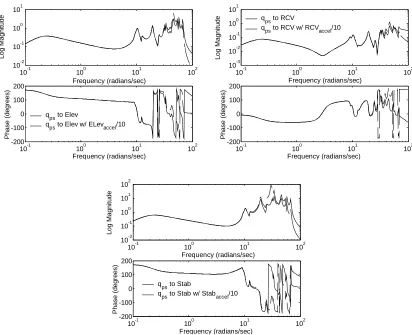
Figure 3.3: Open loop frequency response of pitch rate at the pilot station (qps) and mean axis approximation (qma) responses to control excitation at the back, elevon (solid), and the front, ride control vane (dashed), of the aircraft. ... 49

Figure 3.4: Open loop frequency response of pitch rate at the pilot station (qps) and mean axis approximation (qma) responses to control excitation at the back, all-movable tail (solid), and the front, ride control vane (dashed), of the aircraft 49 Figure 3.5: Open loop frequency response of normal acceleration at the pilot station (nzps) and mean axis approximation (nzma) responses to control excitation at the back, elevon (solid), and the front, ride control vane (dashed), of the aircraft (original response in g’s) ... 50

Figure 3.6: Open loop frequency response of normal acceleration at the pilot station (nzps) and mean axis approximation (nzma) responses to control excitation at the back, all-movable tail (solid), and the front, ride control vane (dashed), of the aircraft (original response in g’s)... 50

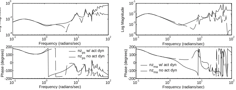
Figure 3.7: Pitch rate dynamics comparison of system with (solid) and without (dashed) actuator dynamics ... 51

Figure 3.8: Normal acceleration dynamic response to elevator excitation comparison of system with (solid) and without (dashed) actuator dynamics (original response in g’s) ... 51

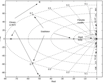
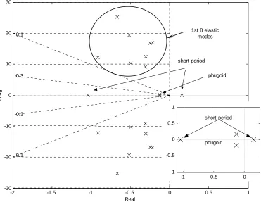
Figure 3.9: Open loop pole locations of a linear system at Mach =0.24 and 1,000 ft, Mass Cruise Final... 52

Figure 3.10: Enlarged area of the linear system above... 53

Figure 3.11: Effect on pitch rate at pilot station of inertial coupling terms of stabilator, elevon, and RCV... 54

Figure 3.12: Effect on normal acceleration at pilot station of inertial coupling terms of stabilator, elevon, and RCV ... 55

Figure 3.13. Third-order actuator model response for original δ and /10δ . ... 56

Figure 4.2: Novel dynamic inversion - introduction of a filter into the inversion loop –

linear case... 64

Figure 4.3: Novel dynamic inversion... 81

Figure 4.4: Short period closed loop poles as a changes ... 82

Figure 4.5: Flexible mode closed loop poles as b changes... 83

Figure 4.6: Novel dynamic inversion with dynamics in the dynamic matrix ( )W x ... 85

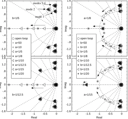
Figure 4.7: Closed loop poles for short period + 1 flexible mode with a changing, b=1/5 ... 86

Figure 4.8: Closed loop poles for short period + 1 flexible mode with b changing, a=1/8 ... 86

Figure 4.9: Longitudinal + 4 modes with a changing... 87

Figure 4.10: Longitudinal + 4 modes with b changing... 87

Figure 4.11: Longitudinal + 1 mode with a changing ... 91

Figure 4.12: Longitudinal + 1 mode with b changing ... 91

Figure 4.13: Closed loop poles for longitudinal + 1 flexible mode with {a,b,∆ζ} constant, ∆ω,vaying ... 95

Figure 4.14: Longitudinal + 1 mode with {∆ω,∆ζ}={-20%, -50%} a changing, b=(1/5, 1/12.5) ... 97

Figure 4.15: Longitudinal + 1 mode with {∆ω,∆ζ}={-20%, -50%} b changing, a=(1/8,1/15) ... 97

Figure 5.1: Sensors and actuators used in the study ... 106

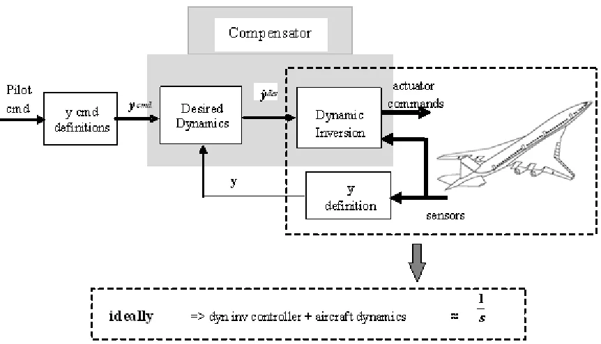
Figure 5.2: Conceptual dynamic inversion control law block diagram... 107

Figure 5.3. Standard vs. Novel dynamic inversion closed loop system. ... 111

Figure 5.4: Pitch rate and nz response to 0.5 stick pitch rate command with no vertical turbulence at pilot station (dashed) and mean axis (solid)... 113

Figure 5.5: Actuator displacement and rate response to 0.5 stick pitch rate command with no vertical turbulence... 113

Figure 5.6: Vertical turbulence in the severe and moderate range for saturated actuators and no saturation cases... 114

Figure 5.7: Pitch rate and nz response to pitch rate command in severe vertical turbulence to 0.5 stick at pilot station (dashed) and mean axis (solid)... 115

Figure 5.8: Actuator response to pitch rate command in severe vertical turbulence to 0.5 stick... 115

Figure 5.9: Pitch rate and nz response to pitch rate command in moderate vertical turbulence to 0.5 stick at pilot station (dashed) and mean axis (solid). ... 116

Figure 5.10: Actuator response to pitch rate command in moderate vertical turbulence to 0.5 stick... 116

Figure 5.11: Pitch rate and nz response to pitch rate command of full stick that saturates controls in severe vertical turbulence at pilot station (dashed) and mean axis (solid) ... 117

xix

Figure 5.13: Pitch rate and nz response to pitch rate command of full stick that saturates controls in moderate vertical turbulence at pilot station (dashed) and mean

axis (solid)... 119

Figure 5.14: Actuator response to pitch rate command of full stick that saturates controls in moderate vertical turbulence... 119

Figure 5.15: Robust stability analysis. (µ lower and upper bounds with µ =1 robust stability boundary) ... 120

Figure 5.16: Pitch rate response at the pilot station to 0.5 stick throw ... 122

Figure 5.17: Pitch rate response at the mean axis sensor to 0.5 stick throw... 122

Figure 5.18: Pitch rate response at the pilot station and measured mean axis of the dynamic inversion controller to 0.5 stick throw ... 122

Figure 5.19: Nz response at the pilot station to 0.5 stick throw... 123

Figure 5.20: Nz response at the sensed mean axis to 0.5 stick throw... 123

Figure 5.21: Actuator surface deflection ... 124

Figure 5.22: Actuator surface rates... 124

Figure 5.23: Frequency response pitch rate at the pilot station to stick input ... 125

Figure 5.24: Frequency response nz at the pilot station to stick input... 125

Figure 5.25: Frequency response of the pitch rate at the pilot station to vertical turbulence ... 126

Figure 5.26: Pole map of the entire 20 mode system with third order longitudinal dynamics. Progressively enlarged sections showcasing different dynamic aspects... 127

Figure 7.1: Trim Conditions ... 180

Figure 7.2: Stability region of (7.8) for variation in control command parameters

(

)

Figure 7.3: Velocity response of nonlinear system and its Taylor series expansions of linear, quadratic, and third-order. Figure on the right is an extract from the left ... 184

Figure 7.4: Angle of attack response of nonlinear system and its Taylor series expansions of linear, quadratic, and third-order. Figure on the right is an extract from the left. ... 184

Figure B1: Symmetric flexible modes of an HSCT vehicle ... 203

Figure B2: Symmetric mode shapes 1 through 5 and their respective frequencies ... 204

Figure B3: Symmetric mode shapes 6 through 10 and their respective frequencies ... 205

Figure C1: Pitch rate response, at mean axis and pilot station sensors, and elevator response to pitch rate command and impulse disturbance in elevator – elastic mode frequency ωe=23.1 rad/sec. ... 208

Figure C3: Pitch rate response, at mean axis and pilot station sensors, and elevator response to pitch rate command and impulse disturbance in elevator - elastic mode frequency ωe=7.7 rad/sec. ... 209 Figure C4: Pitch rate response, at mean axis and pilot station sensors, and elevator

response to pitch rate command - elastic mode frequency ωe=7.7 rad/sec... 210 Figure C5: Pitch rate at pilot station and mean axis to pitch rate command loop frequency

response for 3 different elastic mode frequencies... 212 Figure C6: Pitch rate at pilot station and mean axis to input disturbance loop frequency

response for 3 different elastic mode frequencies... 212 Figure C7: Open loop nominal 3 mode system eigenvalues. Modes enclosed in the box

used for controller design... 213 Figure C8: Sensors and actuators used in the study... 213 Figure C9: Conceptual dynamic inversion control law implementation. ... 214 FigureC10: Pitch rate time response of a 1 mode system with the K1 controller to a half

of a doublet pitch rate command (dashed - at pilot station; solid - at s7). .... 215 Figure C11: Pitch rate time response of a 3 mode system with the K1 controller to a half

of a doublet pitch rate command (dashed - at pilot station; solid - at s7). .... 215 Figure C12: Open loop modal deflection to 2.5 deg elevator command (solid - 3 mode

model; dashed - 1 mode model)... 216 Figure C13: Control law block diagram for a 2 dof dynamic inversion compensator. .. 217 Figure C14: Pitch rate time response of a 1 mode system with the K2 controller to a half

of a doublet pitch rate command (dashed - at pilot station; solid - at s7). .... 218 Figure C15: Elevator (solid) and trailing edge 1+8 (dashed) commanded response to

q_cmd with the K2 controller. ... 218 Figure C16: Gain (10.86dB) and phase (68.23 deg) margins for q_ps/q_cmd... 219 Figure C17: Gain (inf) and phase (72.73 deg) margins for q_s7/q_cmd. ... 219 Figure C18: Robust stability for ζ and ω variation in 1st elastic mode (ζo = 0.0463; ωo =

7.712 rad/sec) (uncertainty: [δζ δω]=[-50% -26%]; solid - (δR+α2δC); dashed -

δC). ... 220 Figure C19: Pitch rate time response of a 1 mode nominal and perturbed systems with the

K2 controller to a half of a doublet pitch rate command, [δζ δω]=[80% -26%]... 221 Figure C20: Nominal 1 mode system with K2 controller pole-zero map... 222 Figure C21: Perturbed 1 mode system with K2 controller pole-zero map [δζ δω]=[80%

-26%]... 222 Figure C22: Pitch rate time response of a 3 mode system with K2 controller to a half of a

doublet pitch rate command (solid - s7; dashed – ps)... 223 Figure C23: Pole zero map of a 3 mode system and effect of the K2 controller on its

elastic modes... 224

Chapter 1 – Introduction 1.1 Motivation

High performance aircraft of the future will be designed to be lighter, more maneuverable, and operate over an ever expanding flight envelope1. This set of

conditions will necessarily mean highly flexible vehicles operating in nonlinear regimes. In order to control these vehicles, new methods are being sought to better optimize their responses to both pilot input and external disturbances, as well as to decrease the cost of vehicle design. Over the last decade, dynamic inversion methodology has gained considerable popularity in application to highly maneuverable fighter aircraft2-5 , as underlying methodology to new generation of highly maneuverable vehicles under development6-9, and might be of benefit to highly flexible aircraft.

The attractiveness of this methodology lies in the fact that the inherent nonlinearities of the problem are explicitly considered. In other words, a nonlinear control law is designed that globally reduces the aircraft dynamics of interest into a set of integrators and, thus, allows one linear controller to provide desired response throughout the flight envelope. This eliminates the need for extensive linearization of the aircraft model for different flight conditions, design of individual controllers for each of these conditions, and finally performing gain scheduling, which is typically an ad hoc and time consuming procedure to link the individual controllers over the flight envelope. Despite these apparent advantages, dynamic inversion is not a panacea of high performance flight control. A number of issues dealing with global system stability and robustness have not been fully addressed. However, the fighter aircraft examples to which dynamic inversion had been applied have shown that this methodology works for current advanced

aircraft2, 3.

One type of aircraft that has gained prominence in recent years is an Uninhabited Aerial Vehicle (UAV). These vehicles span a great variety of missions and hence have a number of very different configurations. One such vehicle is a Helios Prototype designed for very long duration flight, non-stop at least 24 hours at 100,000 ft11. As can be seen from Figure 1.1, the aircraft is an ultra-lightweight flying wing, which is inherently very flexible. The wingspan is 247 ft, longer than the wingspans of U.S. Air Force C-5 military transport (222 ft) or Boeing 747 commercial jetliner (215 ft). The aircraft

recently crashed and an investigation to determine the causes of the control problems that led to the loss of the craft are still in progress.

Figure 1.1: Helios Prototype long duration solar powered flight (courtesy NASA Dryden Flight Test Center).

Furthermore, conceptual combat UAV designs may incorporate highly flexible delta-type wing shapes. The University of Bath and AFRL undertook an

experimental/computational research effort investigating flexible delta wings’ nonlinear aeroelastic response due to unsteady vortex flow12. And in a recent announcement, QinetiQ, the UK’s defense research agency, has designed a flying wing tail-less UAV with no external control surfaces, which uses wing twist and deformation for pitch and roll control. The UAV, called AEUAV-F, applies aeroelasticity to enhance the control power of these controls13. Consequently, in light of all these developments, the question of integrated flight/aeroelastic control assumes great prominence.

dynamics of interest because very extensive development in modeling and simulation has been performed over a number of years and the available models are of very high fidelity. This vehicle class is 300 ft in length with gross weight of 700,000 lbs. The sheer size of this vehicle is put in perspective by a drawing found in Figure 1.2 that places the aircraft on a football field inside a stadium. While this aircraft is not a traditional high

performance aircraft, it does operate over an extensive flight envelope and exhibits elastic characteristics expected of future advanced vehicles. The weight savings produced by lighter materials also result in low frequencies for elastic modes. Generally, these first modes occur around 1.5 Hz (9 - 10 rad/sec) with the first five under 4 Hz, while for a typical subsonic transport this value is 3.2 Hz (20 rad/sec). The implication for this class of vehicles is that the frequency separation between the fastest rigid body dynamics and the slowest elastic mode is less than 10 rad/sec. The lack of separation between rigid and elastic dynamics has significant consequences for flight control and is discussed in detail in later chapters.

If dynamic inversion is to be seriously considered as a methodology for control design of future advanced flexible aircraft, it must be able to deal with the small frequency separation between rigid and elastic modes. Before applying dynamic inversion to a high performance flexible fighter, which includes both elasticity and high performance over an extreme flight envelope, the issue of elasticity must first be

resolved. The HSCT class of vehicles mentioned above offers an opportunity to address elasticity through dynamic inversion while operating under a wide range of aerodynamic conditions but without adding the extra complexity of highly nonlinear post-stall

1.2 Integrated Flight/Structural Mode Control and Dynamic Inversion Literature The state of the art that has bearing on the research presented in this work falls into two separate fields: those of integrated flight/structural mode control and those of dynamic inversion application to aircraft control. The state of the art in dynamic inversion aircraft control is presented first.

1.2.1 Dynamic Inversion Aircraft Control

The application of direct dynamic inversion to aircraft control has reached its peak in open literature with the High Angle-of-Attack Research Vehicle (HARV) project2-5. Subsequent to that project, control involving dynamic inversion changed directions and the methodology became an underlying partner for direct adaptive control with neural networks6, 7. Dynamic inversion has also been used as the underlying methodology for indirect adaptive control to enhance survivability of the next generation of fighter aircraft and implemented online in real-time8, 9. The innovation in both of these methods dealt with adaptively regulating the error in the plant inversion of the rigid vehicles. This new turn did not advance the state of the art of dynamic inversion itself or improve the theoretical underpinning for the methodology beyond that developed in the HARV project, though it has provided some very interesting and useful results in aircraft

adaptive control. Consequently describing the state of the art for dynamic inversion itself is going to focus on the results produced for HARV, summarizing some work on

robustness issues5, and discussing the latest result in global stability for nonlinear rigid aircraft pitch-axis models14.

1.2.1.1 Dynamic Inversion for Aircraft

The nonlinear equations of motion for an aircraft can be written in the control input affine form:

( , )

( ) ( )

x F u x

f x g x u

=

≈ + (1.1)

where x is the vector of state variables and u is the vector of control effectors. It is often desirable to rewrite the above equation in a normal form, which is very useful in

nonlinear systems; but fortunately, for rigid body aircraft dynamics, it can always be completed. Note that any aircraft outputs are a function of the state variables and can be used as the control variables (CV) for (1.1):

( )

CV =CV x

where CV is the vector of control variables. Rewriting the equations in normal form for aircraft is always possible because (1.1) has CVs for the three axes (pitch, roll, yaw), each including a body rate, and control effectors primarily producing torque in the same three axes. However, in review of aircraft application, the original coordinates prove sufficient in considering the problem. Continuing with the idea that CVs are functions of state variables:

( ) ( )

CV CV CV

CV x f x g x u

x x x

∂ ∂ ∂

= = +

∂ ∂ ∂ (1.2)

Let ( )y CV x =h x( ) then (1.2) can be rewritten as ( )

( ) ( ) ( ) ( )

x x

h x

y x h x f x h x g x u

x

∂

= = +

∂ (1.3)

So the dynamic inversion part of the control law appears:

[

]

( ) ( ) ( ) ( )

cmd des

x x

u = h x g x − ⎡_⎣y −h x f x ⎤_⎦ (1.4)

with ( ) ( )h x g x_x invertible for all values of x. For an aircraft with multiple control effectors for a single axis,

(

)

The important generalization to notice is that the number of control effectors must equal the number of control variables. Since three control variables (one for each axis) have a strong angular rate content and conventional aircraft typically have three moment-producing controls (differential ailerons, symmetric horizontal tail, and rudder), this control handles conventional aircraft easily. For an aircraft that has multiple control effectors for a single axis, a method to allocate control requirements to the different effectors is required.

Honeywell was one of the participants and their dynamic inversion based control law was one of several utilized for this program. The HARV flight control is the most detailed, flight-ready set of control laws designed based on dynamic inversion2 that is available in open literature.

The Honeywell design methodology consisted of dynamic inversion for flight control laws. µ-synthesis was employed to determine optimal robust performance for special point cases against which the dynamic inversion based performance was compared. The control laws were analyzed using singular value and µ-analysis techniques. They were also extensively exercised with batch and piloted simulation.

1.2.1.3 Control Law – Basics

The conceptual development of the HARV control laws are presented here because these have become a standard initial starting point for other designs including the one pursued here for flexible aircraft. Some of the reasons for this formulation are elaborated upon in this subsection; some are further discussed in the next subsection.

In general, the control variables are modeled with the differential equations ( , )

y= f u x (1.5)

which depend on aircraft state variables x and the control effectors u. The differential equations are just the rigid body equations of motion. The state variables – roll, pitch, yaw rates, bank angle, angle-of-attack, sideslip, velocity, and flight path angle – are assumed measured (xmeas). The control effectors are aerodynamic surfaces (ua) and thrust vectoring (ut).

A desired rate of change of the control variable is selected to achieve satisfactory handling qualities in response to pilot commands. This is modeled with a first-order differential equation

1

( )

desired cmd meas

y y y

τ

= − (1.6)

with a specified time constant, τ, for each control variable based on the MIL-SPECS16

. The two differential equations for rate of change are then equated which leaves an expression

1

( cmd, meas) ( cmd meas)

f u x y y

τ

to be solved for the control effector commands. Desirable pilot handling qualities are achieved by precompensation of stick and pedal commands, and trim inputs. The pilot inputs are scaled with flight condition dependent gains and a first-order shaping filter to achieve time constants other than those resulting from feedback objectives.

To decrease the sensitivity of the closed loop response to modeling errors and low frequency atmospheric disturbances, integral feedback was incorporated into the desired dynamics without altering the handling qualities as seen by the pilot. With integral feedback, the desired dynamics for the control variables are

2 ( )

2 2

cmd meas cmd meas

c cdt

y= ω ⎡⎢y − y + y −y ω ⎤⎥

⎢ ⎥

⎣

∫

The integral term implies that the control variable will have zero steady state error in response to step commands in the presence of model errors and constant disturbances. Assuming perfect sensors(y= ymeas), the transfer function between ycmd and y is first

order with a time constant given by 2/ωc. Thus, the handling qualities are unaltered from

the first order characteristics of the proportional only feedback.

The value of the proportional feedback of the control variable sets the crossover frequency (ωc) or bandwidth. The bandwidth has an upper limit related to airframe

elasticity such that control action does not excite elastic modes.

Stability of the closed loop system is related to the selection of control variables. In the linear case, closed loop poles are equal to open loop zeros in the transfer function between control effectors and control variables5, 14.

Robust stability consists of basic loop properties that are degraded by high frequency lags; delays; details of the inversion, which depend on control variables and their

complements; and state estimation, if state variables are not measured directly.

Satisfactory basic loop properties are a prerequisite to achieving satisfactory robustness with respect to more detailed assumptions. The basic loop properties are a Bode gain plot that crosses over at ωc with a phase margin of 87 deg. This allows for 42 deg. of phase

whereB_a and B_t are control moment effectiveness divided by inertia; hence, they are dependent on the current state measurements. Control commands are given by

{

}

{

}

1

1 1

lim lim

cmd desired

a a

cmd desired cmd

t t t a a

u B y

u B y B B u

−

− −

=

= − (1.10)

where B_a =B_a unless division by B_a is unacceptable in which case B_a is set to a specified invertible matrix. Reversion to B_a typically takes place when either dynamic pressure is small or angle-of-attack exceeds stall. The control law is intended to operate only when thrust vectoring is available, so B_t is always an inevitable matrix. Note when aerodynamic surfaces are not limited, u_tcmd =0; otherwise, u_t is only required for what cannot be provided by aerodynamic control surfaces. This is essentially known as a daisy-chain method of control allocation. It is necessary to stop the integration of tracking error under limiting conditions to prevent integrator windup.

1.2.1.4 Control Law – Other Aspects

The special HARV linear model used for design assumes the time rate of change of the control variable is a nonlinear function of the measured state plus linear terms in the control effectors. The model subroutine is part of the implementation and computes the function of the state using aircraft equations of motion evaluated at the measured state.

A reduced aerodynamic data base was obtained with a least squares fit for HARV data with assumptions that aerodynamic coefficients are linear in everything except the angle-of-attack and have angle-of-attack dependent multipliers. The accuracy of the fit was deemed acceptable based on the performance and robustness tests of the computed control laws. This aircraft model database, in a sense, replaces the set of gain schedules regarding inner loop feedback gains that is present in existing flight control systems.

modified based on the physics of the high angle-of-attack problem17. Essentially, a “judicious” selection of CVs produced a control law that provided good behavior in all the categories mentioned in the above paragraph for HARV. Of course, the “judicious” selection was based on the physics not only of the aircraft generic relations but also on the specifics of the flight regime of interest.

Another example of dynamic inversion based control laws evaluated in a piloted simulation can be found in Reference 3. The control laws for the F-16 piloted evaluation example were designed based on the HARV report. The control laws produced for the HARV program were used with a change in the aerodynamic database to reflect a different vehicle. It is important to reiterate that, in both cases, the vehicles were described by rigid body equations that were an accurate representation of the physical system in the frequency range of interest, i.e., anything that can be affected by a pilot in combination with external inputs.

The question of robustness and stability were addressed, for both of the design examples, during the control law evaluation using µ-analysis, batch, and piloted simulations. The robustness issues associated with dynamic inversion were addressed more generically in Reference 5. These results are summarized in the next section. 1.2.1.5 Robustness Issues

Good nominal response and well-behaved zero dynamics are not enough for a good control law design. These qualities must also be robust with respect to various modeling errors inherent in aircraft systems. The inversion part of the control law produces the desired dynamics exactly only when f(x) and g(x) are known precisely.

For the rest of this section consider a perturbed model of the aircraft given by

( )( ) ( )

where ∆(s) is an arbitrary stable dynamic perturbation, small for low frequency signals, but increasing in size to unity and beyond as frequency increases. A short derivation shows that the resulting dynamic model for y=CV is then given by

( ) ( ) des

y=CV = δ f −Df + +I D y (1.13)

with

1 1 1

g g− δgg− δg g−

= ∆ + + ∆

D (1.14)

These equations replace the integrators as a new dynamic model for the CVs. Note that there are two major uncertainty terms. The first term, (δ f −Df), is a direct disturbance input to the integrators, while the second term, (I+D)ydes, is a multiplicative perturbation on the control inputs of the integrators. Both terms are correlated through their common perturbation operator D, and all functions in this operator, f, g,δf, and δg, remain dependent on the state vector x.

Note that the new model is still almost linear. Only the perturbation terms are not linear. If this fact is ignored for the moment, well-established design methods are available to construct robust controllers. Perhaps the simplest of these are loop-shaping methods, which satisfy norm-based robustness constraints on the CV-feedback loops 18. If the multiplicative and direct disturbance terms are re-written in terms of Da and Dm,

which are dependent on y and ydes terms, respectively (see Ref. 5 for details), then there are two basic constraints:

(1) sufficient conditions for robust stability with respect to the multiplicative term alone

[

]

1 max

max

1

( ( ) ( )) ( ) ( ) for all ( )

m

I K s P s K s P s s j

D s

σ ω

σ

−

⎡ ₊ ⎤_{< =}

⎣ ⎦ (1.15)

(2) sufficient condition for robust stability with respect to the direct disturbance term alone

[

]

[

]

min (I K s P s( ) ( )) ( ) ( ) max D s P sa for all s j

σ + > σ = ω (1.16)

High-frequency constraints are imposed by the multiplicative term, which requires that the loop be rolled off before the magnitude of Dm(s) exceeds unity. Low-frequency

constraints are imposed by the direct disturbance term, which calls for sufficient low-frequency gain to overpower any destabilizing effects of Da(s). Combining these two

extremes gives the familiar shaping requirements. Whenever the above loop-shaping constraints are widely separated, simple CV compensators suffice like the one employed for HARV aircraft2.

In more challenging situations, when the frequency-domain constraints are tight, the fact that the direct disturbance and multiplicative perturbations occur together and in a correlated way can no longer be ignored. Any of the sophisticated modern multivariable design tools could then be brought to bear to execute the design. Arguably, the most powerful of these is the µ-synthesis method 19, 20.

If the critical assumption of linearity is removed, the formal design options are much less powerful. This occurs because formal norm-based robustness conditions for general nonlinear perturbations are blunt instruments. Consider the following generalization of (1.15) and (1.16), derived from the small gain theorem (see Ref. 5 for more details).

(1) sufficient condition for robust stability with respect to the nonlinear multiplicative form alone

1 1

( )

m

I KP KP

D

−

+ < (1.17)

(2) sufficient condition for robust stability with respect to the nonlinear direct disturbance alone

1 1

( )

a

I KP P

D

−

+ < (1.18)

1

( ) ( ) m g x g x

−

= ∆

D (1.19)

The norm above is equal to the M-peak of the linear actuator/flex perturbation in the control channels of the aircraft and is typically much greater than unity.

Thus, (1.17) can be satisfied only if the M-peak of the CV-loop is much smaller than unity. This requires very small loop gains, i.e., |K(s)P(s)|<<1 for all s=jω. Unfortunately,

such gains cannot satisfy (1.18) because it requires large loop gains to make the M-peak of (1+KP)-1P small enough. Thus, the formal robustness guarantees of the nonlinear theory currently do not help in design.

1.2.1.6 Global Stability Results

One aspect of dynamic inversion concept is the presence of hidden zero dynamics. The zero dynamics15 is a set of system responses that is not observed in the output but is influenced by the control action. They may also present a problem to system

performance if not properly handled.

These dynamics are implicitly defined by the selected CVs and must be examined separately to ensure that they are stable and well behaved. While it is far from trivial to establish properties of zero dynamics globally, local properties obtained from

linearizations are often enough to identify potential problems5.

A recent global stability result for dynamic inversion applied to nonlinear rigid aircraft pitch-axis dynamics appeared in Reference 14 and is summarized in this section. Even though both the airplane model and the control law are somewhat simplified, the result is an important building block for future analysis. The following discussion is to establish under what circumstances can necessary and sufficient conditions for global stability of closed loop system with a dynamic inversion controller hold.

In practice, aircraft stability cannot be expected under all possible flight conditions. For the purpose of analysis, two different sub problems of stability are considered:

1. assume unlimited control authority and work globally, or

2. restrict attention to a subset of the states on which control authority is adequate. In what follows, only the first sub problem, i.e., the discussion of global results, is considered.

The control problem can be stated as follows:

Given an equilibrium state x, determine a controller u=K(x,x) so that x is a global attractor for the system

( , ( , ))

x= f x K x x (1.20)

Any global attractor must be an equilibrium state. This problem is addressed using dynamic inversion for vehicle models having a unique equilibrium point for appropriately chosen engine thrust, T.

The approach is to invert the rotational degrees of freedom to a set of stable, second order dynamics. The steps include constructing controller K, showing stability of the attitude dynamics, and addressing the stability of zero dynamics. A desired stable set of second-order linear dynamics for θ is

2

2 ( )

cmd cmd

q = − ξωq−ω θ θ− (1.21)

With this controller, the closed loop dynamics decouple into velocity dynamics (U,W) given by

, 2

, ,

sin( ) 1 /

cos( ) 2 ( ) 0

x y cmd x

z M

z

C I q

Wq g C T m

U

V S

C

Uq g m C cmC

W

δ δ δ

θ

ρ

θ α

− − ⎡ ⎤ ⎡ ⎤

⎡ ⎤ ⎡₌ ⎤ ⎡₊ ⎤_{+ + +}⎡ ⎤

⎢ ⎥ ⎢ ⎥

⎢ ⎥ ⎢ ⎥ ⎢ ⎥ ⎢ ⎥

⎣ ⎦ ⎣ ⎦ ⎣ ⎦

⎣ ⎦ ⎣ ⎦ ⎣ ⎦ (1.22)

and attitude dynamics (q,θ) given by

2

2 ( )

1 0

cmd

q

q

ξω ω θ θ

θ

⎡ ⎤

−

⎡ ⎤ ⎡₌ ⎤ − −

+ ⎢ ⎥

⎢ ⎥ ⎢ ⎥

⎣ ⎦ ⎣ ⎦ ⎣ ⎦ (1.23)

The dynamics of the attitude loop, (q,θ), have been reduced to linear by dynamic inversion and converge to (0,θcmd).

of initial and transient state conditions. The global stability result that follows provides an explanation for the above observations.

Theorem14: Assume that 1. the total drag coefficient

,

,

( )

( ) ( ) ( ) 0

( ) M

D D D

M

C

C C C

C

δ

δ

α

α α α

α

= − > (1.24)

2. the aerodynamic function satisfy the dissipative condition

3C_D( ) dCL( ) 0

d

α α

α

+ > (1.25)

3. for a given T and cmd, the following equation of

sin( _cmd) _z( ) cos( _cmd) _x( ) 0

T

C C

mg θ α θ α

⎛ ⎞

− − =

⎜ ⎟

⎝ ⎠ (1.26)

has only one solution α= α*.

Then, for a given T and θcmd, the closed loop system (1.22)-(1.23) has a unique equilibrium (θ*,q*,U*,W*) given by

, 0 cmd q θ∗₌θ ∗ ₌

and

2 cos( ) 2 cos( )

* cos( *), * sin( *)

( *) ( *)

cmd cmd

z z

mg mg

U W

SC SC

θ _α θ _α

ρ α ρ α

− −

= = (1.27)

where α* is the unique solution of (1.26).

Moreover any solution (θ(t), q(t), U(t), W(t)) of the closed loop system (1.22)-(1.23) satisfies

( )t _cmd, ( )q t 0, ( )U t U*, W t( ) W*

θ →θ → → →

as t→ ∞. That is to say (θcmd,0,U*,W*) is a global attractor of the closed loop system (1.22)-(1.23).

Now return to the question of stability of zero dynamics of the closed system (1.22). In the linear case, the issue of stability is related to right half plane zeros in the elevator to pitch angle transfer function. This transfer function has two such zeros21 and under typical flight conditions for rigid body aircraft, these are both minimum phase. It has been mentioned in Reference 5, as well as in Reference 14, that the zeros of open loop plant become poles of the closed loop system when dynamic inversion is employed. This result has been both observed in practice2, 5, including present work, and shown

mathematically14.

The stability robustness of the above result to uncertainty in the aerodynamic coefficients must be analyzed. If no uncertainty on the pitch moment exists, then the dynamics of the pitch attitude and the pitch rate are still decoupled from those of the velocities. The stability results for the nominal aerodynamic functions work immediately for the perturbed CL, CD, CL,δ and CD,δ. This generalization is significant because it is the

first result obtained for robustness of nonlinear dynamic inversion control laws for rigid fighter aircraft.

1.2.2 Integrated Flight/Structural Mode Control

The state-of-the-art for the second major issue for the research problem is discussed in this section. Since initial development and deployment of the B-1 bomber, which served as the most recent aircraft where structural modes had to be actively controlled, integrated flight/structural mode control (SMC) received limited coverage in open literature. The primary reason for this is unavailability of reasonable fidelity models that are not proprietary. In fact, the high fidelity HSCT model used as a proving ground for the research presented is restricted, though the results obtained with it are now

publishable. Hence, the work in this area, until very recently, has concentrated in those agencies and companies that deal with the next generation of supersonic transports and had access to good models (Aerospatiale, Boeing, NASA). Very recently, an interest in this area has reemerged with the advent of different types of UAVs under consideration and will be addressed later in this section.

mode dynamics. The first fuselage bending mode for the B-1 is at 18 rad/sec (2.8 Hz)22, which makes the rigid body flexible dynamics separation considerably larger than that for an HSCT-type vehicle. The structural mode control system developed for the B-1 was the first of its kind in that it actively managed the flexible dynamics. One of the

requirements for this system was that it was to be installed on top of an already existing flight control system and would not interfere with it in any way. Since the system was installed to provide a specific level of ride quality to the crew, the requirement of noninterference with flight control and the design of the two systems separately were consistent with the objective and the dynamics of the aircraft. This approach, while not optimal, was adequate for aircraft displaying the dynamic separation between rigid and flexible dynamics of the B-1. However, as discussed in later chapters and as been confirmed by other researchers23, 24, the unprecedented small separation between rigid body and flexible modes of the HSCT type vehicle would make this approach completely inadequate. Briefly the reasons for this are that the desired flight controller bandwidth, to satisfy the flying qualities criteria, has less than a decade frequency separation with the first elastic mode. Furthermore, compromising and reducing the controller bandwidth would still result in insufficient roll off to attenuate flexible mode excitation. The elastic modes themselves are too closely spaced to make notch filters, a popular device for vehicles with large dynamic separation and only one or two modes in need of attenuation, an attractive option. The HSCT vehicle is roughly 2.5 times the size of the B-1 (see Fig. 1.3), which partially accounts for the differences in flexible dynamics, but the similarity in shape also foreshadows the similar control problems.

A step towards integrated flight/SMC was taken in Reference 25 where quantitative feedback theory was used for design of a longitudinal pitch-axis flight control system for a highly flexible B-1 type vehicle. The aircraft model utilized in this work was an

Figure 1.3: HSCT size comparison with B-1.

Work on an integrated flight/SMC control for a highly flexible aircraft with significant cross coupling between flight mechanics and flexible modes appeared in Reference 26. Based on the published open loop poles, the vehicle under consideration was indeed an HSCT class vehicle. The model used for control design and analysis was linear and consisted of the longitudinal rigid body model linearized about a steady-state condition and the aeroelastic model that includes aerodynamic lag terms, τ, (a general discussion of aeroelastic models follows in Chapter 3). These two models are coupled by connecting their respective measured outputs at the same structural points on the aircraft. The combined model is given by

[

]

[

]

[

]

0

where ,

r r r r

q

e e e e

r

r e r e q

e

T _T

r e

x A x B

x A x B

x

y C C D D

x

x V q nz x

y nz q nz

δ δ

α θ η η τ η η τ

⎛ ⎞ ⎡ ⎤⎛ ⎞ ⎡ ⎤

= +

⎜ ⎟ ⎢ ⎥⎜ ⎟ ⎢ ⎥

⎝ ⎠ ⎣ ⎦⎝ ⎠ ⎣ ⎦

⎛ ⎞

= _{⎜ ⎟}+ +

⎝ ⎠

⎡ ⎤

=_{⎣ ⎦} =

⎡ ⎤

= ⎣ ⎦

∫

∫

…

(1.28)

stability and output feedback that tries to recover this performance. The full state feedback LQR is used on the combined rigid/elastic model and the performance index weighting matrices are manipulated to place rigid body poles into an eigenspace that would provide the desired performance. The resulting controller would then provide rigid body performance compatible with flexible mode stability. The next step is to obtain an output feedback controller whose resultant closed loop dynamics are as close as possible to the ones produced by the LQR. The approach chosen to produce this output controller is the constrained minimization of the difference between the actual and desired eigenstructure produced by LQR

1

min max

P

des i i i

i F

J p

K K K

λ λ

=

= −

< <

∑

(1.29)

where pi are scalar weights, and constraints on K are defined for practical consideration

of gain scheduling. The results for the model in (1.28) do provide stable pitch rate and normal acceleration response free of significant flexible mode dynamics to 0.1 g

command. However, the model does not reflect the inherent complexity of dynamics for the aircraft with cross coupling between rigid body flight dynamics and structural

dynamics so the proposed control technique cannot be adequately evaluated.

y1 (q_ps)

y2 (q_meas)

y3 y2cmd

(q_cmd)

K₂₂(s)

K₁₁(s) K₂₁(s) K₁₂(s)

A_δelev(s)

A_δrcv(s)

G(s) P₂(s)

y_stick

δrcv_c

δelev_c

-+

+

+ + +

Figure 1.4: Multi-loop control law architecture.

command shaping filter, Aδ(s) are actuator dynamics, G(s) is the plant, and Kij(s) are

individual dynamic filters. In the final result the Kij(s) filters are 3rd, 3rd, 3rd, and 4th order

respectively with a 4th order command prefilter P2(s).

The model used for design and analysis of this controller was similar to the one discussed in this work and is based on the integrated rigid/structural mode dynamics, though necessarily linearized for application of this methodology. The controller simulation results are very favorable in response to small input commands and provide good robustness to gain and phase perturbations in individual loops. Here the difficulty in designing all of the dynamic filters and command prefilter is balanced by a classical controller architecture. This methodology presents a potential linear alternative to the novel dynamic inversion methodology explored in this work.

based on the measured output, the regulated output, and the model inversion error. As in other adaptive control methods that utilize model inversion error and then use an adaptive neural network law to drive that error to zero6, 29, this attempts to do the same but it lacks the inversion error since the structural model is unknown. This inversion model error is provided by an adaptive observer described in detail in Reference 30. At this stage, this approach is a candidate approach to either reducing the dependence of existing design on structural model filtering or eliminating the need for structural filtering in the future design altogether.

1.3 Contribution of This Work

The contribution of this work to the state of the art is predicated on the development and application of dynamic inversion methodology to handle highly flexible aircraft in an integrated flight/structural mode control manner. The development and evaluation are performed on a sophisticated, high fidelity, nonlinear dynamic model across the frequency spectrum. The dynamic nature of structural modes and the flight control reciprocal interaction with flexible modes because of unprecedented small separation between rigid body and flexible modes are the key elements of the aircraft model. An innovation to the standard methodology of dynamic inversion has been introduced in the manner described in this work to accommodate the nature of the vehicle and fulfill the dual objectives of integrated flight/SMC control. These objectives constituted command following, disturbance rejection in the rigid body, improved structural dynamic damping to minimize excitation from turbulence, and rendering the aircraft rigid from the pilot station perspective.

potentially destabilizing effect of pole cancellation close to the jω-axis in case of modeling uncertainty.

The structural nature of the modification to the standard dynamic inversion

methodology and its effect on the necessary level model complexity for design has been established with particular attention given to establishing physical understanding of the control design process. Furthermore, the effect of uncertainty in the structural mode dynamics has been addressed as well.

Further contribution is addressing the issue of dynamic inversion and stability of highly flexible aircraft studied in this work from the mathematical perspective. The approach is rather straight forward. The vehicle driven by a controller must reach some equilibrium whose stability must be evaluated. The results show how assessing stability of an n-dimensional system can be reduced to checking stability of a two-dimensional one using algebraic expressions that are based on the vehicle characteristics such as aerodynamic coefficients. This reduces a complicated dynamical problem to something purely algebraic and manageably complex. The results presented are the first to include flexible dynamics in stability analysis of the dynamic inversion methodology. These form an initial basis to more complicated control problem formulation that includes the novel dynamic inversion methodology employed to design an integrated flight/SMC controller for a high fidelity model discussed earlier. The changes in dynamics attributed to the innovation in the inversion methodology are explored for both linear and nonlinear systems. This work has added to both analytical and physical insight regarding the nature of novel dynamic inversion applied to an integrated flight/structural mode control for a high flexible aircraft.

Furthermore, a new tool is introduced in an attempt to systematically find Lyapunov functions that would guarantee local stability for the nonlinear system with the novel dynamic inversion controller alluded to above. The tool, called SOSTOOLS, is based on the Sum of Squares decomposition for finding a Lyapunov function algorithmically.

1.4 Organization of the Thesis

This dissertation is divided into eight chapters each addressing a major component of the work. There are also five appendices each containing important information and results pertinent to the main results but not central to them. The chapters are divided as follows. Chapter 2 provides a brief overview to the dynamic inversion, discussing

necessary background for a reader who might not be familiar with the technique. Chapter 3 concentrates on the development of the sophisticated, high fidelity, nonlinear dynamic model of the highly flexible aircraft across the frequency spectrum. The development touches on the general unsteady aerodynamic influences on the structural modes and how his was incorporated in to the standard aircraft equations of motion that retained the reciprocal dynamic rigid body and flexible dynamics. The open loop nature of the vehicle class model such way is also presented.

Chapter 4 introduces the novel dynamic inversion methodology in detail and explores the influence it has on the closed loop system dynamics. The design and evaluation of the control law based on this methodology in the high fidelity, full nonlinear simulation in the presence of turbulence and flexible mode uncertainty is discussed in Chapter 5. Chapter 6 continues the analysis with theoretical stability result concerning dynamic inversion and highly flexible aircraft. Chapter 7 touches on newly evolving methodology of proving stability by finding Lyapunov function based on sum of squares and applying this methodology to the problem at hand. Finally, Chapter 8 contains the conclusions and suggestions for further research.

Chapter 2 – Introduction and Background to Dynamic Inversion 2.1 Introduction

Dynamic inversion, also known as feedback linearization, fundamentally is an algebraic transformation of a nonlinear system dynamics into a fully or partially linear and controllable one, so that linear control techniques can be applied. It deals with techniques for transforming original system models into equivalent models of a simpler form. The central premise of dynamic inversion control methodology is based on the idea that control effector commands are a sum of signals from essentially two different controllers that together comprise what is commonly known as a dynamic inversion controller. One part of the controller is based on the nonlinear model of the system and generates commands that would cancel the nonlinearities and make the actual system behave in the manner of first order linear dynamics, typically an integrator. The other part of the controller is linear in nature and issues commands that make the linear dynamics behave in a desired way. This linear controller is ideally the same throughout the region of interest, but in practice may be divided into two or three parts each

representing a distinct dynamic regime for better system performance. It is designed as any linear controller to provide robustness for dynamics mismatch between the nonlinear system model and the actual system dynamics. The robust performance analysis on the entire dynamic inversion controller can be conducted at different flight conditions using a very powerful linear technique of µ-analysis. However, since the controller is nonlinear in nature and spans the entire flight envelope, one would like to perform analysis that would guarantee stability in the entire operating regime. Part of the current work proposes such a stability test.

A number of references give details on the underlying theory and methodology of dynamic inversion15, 34. The brief overview in this chapter provides important highlights that should facilitate the motivation behind the research presented.

2.2 Dynamic Inversion Brief Overview 2.2.1 Input-Output Linearization: SISO Case

( , ) ( ) ( ) , ( )

n

x F x u f x g x u x u

y h x y

= ≈ + ∈ ∈

= ∈ (2.1)

In order to produce an input-output controller, an explicit relationship between input u

and output y must exist. At this point the notion of relative degree must be introduced. Informally, relative degree r is defined as exactly equal to the number of times one has to differentiate the output y(t) at t=to in order to have the value of u(to) of the input explicitly appearing. In a linear system this is equivalent to the difference between the number of poles and zeros. A system with a relative degree defined in some neighborhood of xo allows us to transform the nonlinear system into the normal form. Prior to giving a formal definition of relative degree some mathematical tools need to be defined.

Definition: Let h: n → be a smooth scalar function, and f : n → n be a smooth vector field on n, then the Lie derivative of h with respect to f is a vector field defined by

( ) ( )

f

h

L h x f x

x

∂ =

∂

Thus, the Lie derivative L h_f is simply a directional derivative of h along the trajectories of the systemx= f x( ). The new notation is convenient for repeated calculation of the derivative with respect to the same or a different vector field. For example, repeated Lie derivatives can be defined recursively

0

( ) ( ) f

L h x =h x

1

1 ( )

( ) ( ) ( )

k f

k k

f f f

L h

L h x L L h x f x

x

−

− ∂

= =

∂

Similarly, if g is another vector field, then the scalar function L L h x_{g f} ( ) is ( ( ))

( ) f ( )

g f

L h x

L L h x g x

x

∂ =

∂