www.hydrol-earth-syst-sci.net/12/727/2008/ © Author(s) 2008. This work is distributed under the Creative Commons Attribution 3.0 License.
Earth System
Sciences
On the measurement of solute concentrations in 2-D flow tank
experiments
M. Konz1, P. Ackerer2, E. Meier3, P. Huggenberger1, E. Zechner1, and D. Gechter1
1University of Basel, Departement Umweltwissenschaften, Switzerland
2Universit´e Louis Pasteur, Institut de M´ecanique des Fluides et des Solides, CNRS, UMR 7507,Strasbourg, France 3Edi Meier & Partner AG, Winterthur, Switzerland
Received: 30 October 2007 – Published in Hydrol. Earth Syst. Sci. Discuss.: 20 November 2007 Revised: 8 April 2008 – Accepted: 9 April 2008 – Published: 14 May 2008
Abstract. In this study we describe and compare
photomet-ric and resistivity measurement methodologies to determine solute concentrations in porous media flow tank experiments. The first method is the photometric method, which directly relates digitally measured intensities of a tracer dye to so-lute concentrations, without first converting the intensities to optical densities. This enables an effective processing of a large number of images in order to compute concentration time series at various points of the flow tank and concentra-tion contour lines. This paper investigates perturbaconcentra-tions of the measurements; it was found both lens flare effects and image resolution were a major source of error. Attaching a mask minimizes the lens flare. The second method for in situ measurement of salt concentrations in porous media ex-periments is the resistivity method. The resistivity measure-ment system uses two different input voltages at gilded elec-trode sticks to enable the measurement of salt concentrations from 0 to 300 g/l. The method is highly precise and the ma-jor perturbations are caused by temperature changes, which can be controlled in the laboratory. The two measurement approaches are compared with regard to their usefulness in providing data for benchmark experiments aimed at improv-ing process understandimprov-ing and testimprov-ing numerical codes. Due to the unknown measurement volume of the electrodes, we consider the image analysis method more appropriate for in-termediate scale 2D laboratory benchmark experiments for the purpose of evaluating numerical codes.
Correspondence to: M. Konz ([email protected])
1 Introduction
Laboratory experiments are an excellent way of providing data to develop transport theories and validate numerical codes. They have several advantages: boundary and ini-tial conditions are known, the porous medium properties can be defined separately and the experiments can be repeated if necessary. Excellent reviews of mass transfer in porous media at the laboratory scale can be found in Silliman et al. (1998) and Simmons et al. (2002). A variety of meth-ods exists for qualitative and quantitative determination of solute transport in porous media experiments. Tradition-ally this is done by intrusive methods where extracted flu-ids are analyzed in the laboratory (e.g. Swartz and Schwartz, 1998; Barth et al., 2001). These methods are work intensive and require a well-equipped laboratory for chemical analy-sis. Further, the temporal and spatial resolution of concen-tration determination is limited due to point sampling, and perturbations of the flow field cannot be excluded. Oost-rom et al. (2003) introduced the non-intrusive dual-energy gamma radiation system methods for 3D experiments. Os-wald et al. (1997) and OsOs-wald and Kinzelbach (2004) used the nuclear magnetic resonance (NMR) technique to derive concentration distributions of 3D benchmark experiments for density dependent flow. This method is very precise but it is limited to small flow tank experiments due to the size of the NMR tomograph.
al., 1993; Swartz and Schwartz, 1998; McNeil et al., 2006; Goswami and Clement, 2007).
Reflected light is used for image analysis in most interme-diate scale experiments (e.g. Oostom et al., 1992; Swartz and Schwartz, 1998, Wildenschild and Jensen, 1999; Simmons et al., 2002; Rahman et al., 2005; McNeil et al., 2006; Goswami and Clement, 2007). The advantage of this technique is that it can be used with non-transparent porous media material, e.g., sand and with thick flow tanks that prevent light trans-mission. However, the use of reflected light to quantify dye concentrations can lead to problems with image noise, re-flected and diffusive light from surroundings and can there-fore alter the image quality. A promising alternative is the light transmission technique to measure emitted light from behind the flow tank opposite the light source (e.g. Corap-cioglu et al., 1997; Detwiler et al., 2000; Huang et al., 2002; Theodoropoulou et al., 2003; Jones et al., 2005). Catania et al. (2008) provide an excellent literature review of trans-missive experiments and data processing techniques. These studies used very thin small-scale flow models of maximum 1 cm thickness, which enable light transmission.
Variations in lighting, exposure and film development re-sult in non-uniform image intensities between successive im-ages. Rahman et al. (2005) used theγ-calibration model to correct the color representation of images (Icorr):
Icorr=a+b·Iγ (1)
wherea, bandγ are correction parameters, assumed to be spatially uniform, andI is the measured intensity. The val-ues of the parameters are determined by fitting the measured intensities of color cards to the ideal model. Schincariol et al. (1993) and McNeil et al. (2006), amongst others, convert the measured intensities to optical density. Optical densityD
is non-linearly related to intensityI by:
D=log10(a/I ) (2)
wherea is a constant of proportionality. This involves the optimization of intensity vs. optical density standard curve of each image to be investigated and an optimization of op-tical density vs. concentration standard curve. However, the conversion of intensity to optical density or the application of theγ-calibration model is only necessary if:
1. Analogue images are taken and the film has to be devel-oped and scanned to convert the image to digital data ; 2. Automatically, non-linearly adjusted and compressed
images are used.
If only the spatial evolution of plumes at a limited number of timesteps is investigated, the computational efficiency is of minor importance because the intensity vs. optical density standard curve has to be optimized only for a small number of images. For the evaluation of numerical codes however, breakthrough curves at distinct points with a high temporal
resolution are necessary. This requires processing of a large number of images and the computational efficiency becomes a significant criteria. As opposed to Schincariol et al. (1993), Swartz and Schwartz (1998) and McNeil et al. (2006) we re-late linearly measured intensities directly to concentrations without standardization to optical densities to enable pro-cessing of a large number of images with the aim of deriving breakthrough curves of a high temporal resolution. In this study, we apply the light reflection technique because the back wall of our flow tank holds devices for measuring re-sitivity and pressure, which preclude the use of a light trans-mission technique. The light reflection technique is more appropriate if experiments are done with porous media that is more opaque then glass beads such as clayey inclusions and lenses. Therefore, this study aims to provide details on this technique. We investigate the impact of image resolution (pixels per length) on the precision of the results, and the im-pact of lens flare on intensity measurements. In the literature on photometric measurements of plume distribution in flow tanks, little attention has been paid to errors in concentration determination caused by these effects.
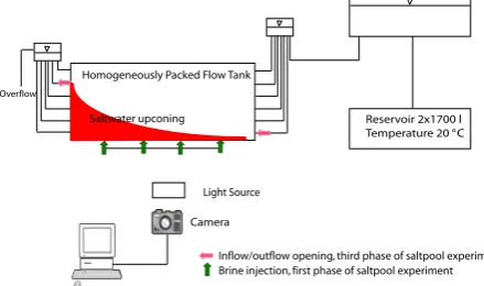
Light Source
Camera Homogeneously Packed Flow Tank
Reservoir 2x1700 l Temperature 20 °C
Inflow/outflow opening, third phase of saltpool experiment Brine injection, first phase of saltpool experiment
Overflow
[image:3.595.309.546.63.193.2]Saltwater upconing
Fig. 1. Schematic experimental setup.
2 Description of the experimental setup
The flow experiments were conducted in a Plexiglas tank with the dimensions (L×H×W) of 1.58 m×0.6 m×0.04 m (Figs. 1 and 2). The back of the tank holds measurement instruments, such as pressure sensors, electrodes of the resis-tivity measurement cell system (RMC) and temperature sen-sors. The front side of the tank consists of a clear Plexiglas pane facilitating visual observation of the tracer movement through the homogenous porous medium during the course of the experiments. The tank has four openings at the bot-tom, which are regulated by valves. Another six openings each are placed at the left and right side of the tank. These openings are also regulated by valves and connected to fresh-water reservoirs. The height of the reservoirs can be adjusted to adapt the velocity of the water inside the porous media. Two 1700 l deionized freshwater reservoirs, where the water temperature is kept constant at 20◦C to avoid degassing in the porous media, maintain water supply to the inflow reservoir. Tension pins with a diameter of 0.5 cm were installed within the tank to prevent the deformation of the Plexiglas wall. Be-cause these obstacles are minor, we assume that they do not perturb the flow. Glass beads with a diameter of 0.6 mm were used as a porous media. The tank was homogenously packed. During filling, there was always more water than glass beads in the tank in order to avoid air trapping. A neoprene sheet and air tubes were placed between the Plexiglas cover and the porous media. The air tubes can be inflated to compensate for the free space when the glass bead settles, preventing prefer-ential flow along the top cover of the tank. A supplementary experiment with traced water and horizontal flow conditions revealed that there are no preferential pathways and that the water flows homogenously through the porous media.
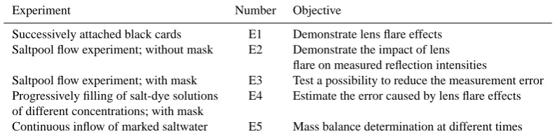
Five different experiments were conducted in order to as-sess the image analysis methodology and the resistivity mea-surement system. Table 1 summarizes the experiments. In the first experiment E1, we successively placed black cards on the front window of the tank to demonstrate the lens flare effect (Sect. 3.5). E2 and E3 are density-dependent flow
ex-Fig. 2. Tank of E3 with mask to reduce effects of flare and filling levels of E4.
periments using red dyed saltwater with a density of 1063 g/l. The experiments E2 and E3 in Table 1 (Sect. 3.5) consisted of four phases. The brine with an initial concentration of 100 g/l was marked with 1 g/l of the red food dye Cochineal Red A (E124). In the first phase of the experiment, the brine was pumped into the domain from four openings at the bottom of the tank, as indicated in Fig. 1 by the green arrows. Buoy-ancy effects forced the brine to move laterally in the second phase and form a planar brine-freshwater interface. No flow was applied in this second phase through any openings in the tank. At the end of this phase, the brine had equilibrated with a mixing zone of about 4 cm above 3 cm of brine with the initial concentration of 100 g/l. The head difference between inflow and outflow reservoirs generated a constant flow dur-ing the third phase of the experiment, which we refer to in the following as the flow phase. Flow through the inflow opening on the lower left side of the tank (11 cm above the ground, red arrow in Fig. 1), close to the brine and the outflow opening on the upper right side of the tank (45 cm above the ground, red arrow in Fig. 1), forced an upconing of the saltwater be-low the outlet as shown in Fig. 1. Mechanical dispersion and advection processes cause the upconing of the saltwater. The last phase is the calibration phase to enable the conversion of dye intensities to concentrations, (for details on this phase see Sect. 3.4).
[image:3.595.50.270.66.196.2]Table 1. Experiments conducted to assess the image analysis technique and the resistivity measurement cell (RMC) technology.
Experiment Number Objective
Successively attached black cards E1 Demonstrate lens flare effects
Saltpool flow experiment; without mask E2 Demonstrate the impact of lens
flare on measured reflection intensities
Saltpool flow experiment; with mask E3 Test a possibility to reduce the measurement error
Progressively filling of salt-dye solutions E4 Estimate the error caused by lens flare effects
of different concentrations; with mask
Continuous inflow of marked saltwater E5 Mass balance determination at different times
3 Concentration determination with photometry
3.1 Image acquisition and general concept of optical con-centration determination
The dense fluid was marked with a dye to visually differen-tiate the saltwater from the ambient pore water. Cochineal Red A (E124) was used as tracer. This food dye is non-sorbing, nonreactive with NaCl in concentrations used for the experiment (Rahman et al., 2005 and our own batch ex-periments). Photometric analysis of different dye-saltwater solutions revealed that there is no degradation or optical de-cay of dye over a period of up to 7 days. Different diffu-sivity could cause separation of dye and saltwater leading to erroneous concentration determinations. In the literature other authors have used various dyes, including food color, to track the movement of dense saltwater in laboratory-scale aquifer models. Neither Schincariol et al. (1993), Swartz and Schwartz (1998) nor Goswami and Clement (2007) re-ported difficulties due to dye-salt separation. The latter used a red food color comparable to Cochineal Red A. We con-ducted column experiments (1 m length) with different salt-dye solutions and compared breakthrough curves of salt and colour. The salt concentrations were measured using stan-dard resistivity cells (WTW) and the color concentrations were determined using a spectrometer (Shimadzu UV-1700 Pharma Spec). No separation could be observed. Further-more, differences in the diffusivity are of minor importance in experiments dominated by advection as is the case in our experiments.
To determine concentration distributions in the tank, we took photos with a digital camera (Nikon D70) using a re-producible illumination with a single light source placed right above the camera at a distance of∼3 m from the tank. The light source (EKON JM-T 1×400 W, E40) was adjusted and checked with a luxmeter to minimize spatial lightning nonuniformity. However, it was not possible to totally avoid lightning nonuniformity and a higher intensity remains in the center of the photographed domain. White, grey and black cards were attached on the front pane of the tank (Fig. 2). A dark curtain placed around the entire experimental setup
prevented reflections of any objects on the tank pane. Fur-thermore, in order to avoid lighting nonuniformity due to daylight, there were no windows in the laboratory. All cam-era parameters were set manually (shutter speed 1/8 s, aper-ture 13.0, ISO200). For image processing it is important that images, taken at different times, match on a pixel-by-pixel basis. A computer programme (Nikon camera control-PRO) controlled the camera, which was not touched or re-moved during the entire experiment including the calibration procedure. Therefore, neither rotation nor translation of im-ages is necessary. The digital camera stores linear raw data (.nef) beside the automatically non-linearly processed photos (.jpg). Raw data is the output from each of the original red, green and blue sensitive pixels of the image sensor, after be-ing read out by the array electronics and passbe-ing through an analogue-to-digital converter. A linear development means that no gamma correction has been applied yet, and thus lev-els are distributed along the histogram in a linear way being each of them proportional to the amount of light (number of photons) that the pixel was able to capture during the ex-posure. The used converter, dcraw, generates linear 16-bit tiff images from the raw data The 12-bit information gained from the camera is linearly spread along the 16-bit of the tiff image. This was necessary because standard PC systems either work on 8- or 16-bit but not on 12- bit. 16- bit was taken to preserve the information of the 12- bit data (e.g. http: //www.guillermoluijk.com/tutorial/dcraw/index en.htm).
The image-processing procedure includes the following steps: (1) data converting to 16 bit tiff images (65536 inten-sity values per channel of the RGB color space) with the free-ware dcraw (http://cybercom.net/∼dcoffin/dcraw/), (2)
3.2 Correction of fluctuations in brightness (Step 3) A constant light source is difficult to achieve because of fluc-tuations in energy supply. The first four graphs in Fig. 3 show the intensities of attached white, grey and black cards (see Fig. 2 for the position of the cards), which are strongly influenced by the fluctuations in lightning. The spikes in the raw data (first four graphs) could be caused by fluctua-tions in electricity supply. The intensities shown in the figure were recorded over two days including the night. 0–600 were taken in the evening and overnight, whereas 600 onwards are images taken in the morning and over the day. This could ex-plain the increased fluctuations in energy supply during the day. Existing methods of image processing convert measured intensities into optical densities based on intensity vs. op-tical density standard curve in order to correct fluctuations in brightness. The reference values of optical density are taken from the attached grey scales. This step is necessary if the raw data are non-linear because analogue photography is used and the photos are developed and scanned, or automati-cally pre-processed images are taken. Due to the linearity of our raw data, neither theγ-calibration model (Rahman et al., 2005) nor the translation to optical density (e.g. Schincariol et al., 1993) to correct fluctuations in brightness is neces-sary. The fluctuations can be corrected (Icorr(i, j )) using the
attached upper white card as reference value (Iref)for each
image:
Icorr(i, j )=I (i, j )/Iref (3)
The last three graphs in Fig. 3 show how the correction method works for the lower white card, the grey and the black cards (Fig. 2). We tested this approach for several points on the tank located not only in the center of the tank but also in the corner of the domain where illumination differences between the reference white and the observation points are highest. The method performs well at all observation points. As a consequence, the images are on the same intensity level after the correction step, and changes in intensity do result only from changes in dye concentration and not from fluc-tuation in lightning. Minor flucfluc-tuations still persist and are related to scattered reflection on the camera lens, which can-not be corrected. These uncertainties are treated in the error estimation in Sect. 3.6.
3.3 Impact of optical heterogeneity of porous media and determination of measurement area (Step 4)
The resolution of the images is crucial, especially in exper-iments where concentrations vary spatially with a steep gra-dient, e.g., in transition zones. In the literature, little atten-tion has been paid to analyzing the impact of the resoluatten-tion on the precision of the derived concentration data. Schin-cariol et al. (1993) suggested a general median smoothing (3×3 pixels) to reduce noise from bead size. The image res-olution of our digital images (approx. 0.31 mm2/pixel)
im-Raw Intens ity (-) 24000 26000 28000 30000 32000 34000 36000 Raw In te ns ity ( -) 30000 32000 34000 36000 38000 40000 42000 R aw In te ns ity ( -) 6500 7000 7500 8000 8500 9000 Raw Intens ity (-) 3000 3200 3400 3600 3800 4000 4200 R aw In te ns ity ( -) 1.176 1.178 1.180 1.182 1.184 1.186 1.188 1.190 1.192 R aw In te ns ity ( -) 0.254 0.255 0.256 0.257 0.258 0.259 Pictures
0 100 200 300 400 500 600 700 800 900 1000
Ra w In tens ity ( -) 0.1170 0.1175 0.1180 0.1185 0.1190 0.1195
Upper white card
Lower white card
Grey card
Black card
Lower white card corrected with upper white card
Grey card corrected with upper white card
[image:5.595.311.543.59.330.2]Black card corrected with upper white card
Fig. 3. Measured and processed intensity values of grey and black cards.
plies a high resolution of the concentration determination at a point. In order to assess the impact of resolution, we filled the tank with solutions of different concentrations, took im-ages of each solution and analyzed the intensity distributions in squares of 25 cm2 (8281 pixels) at different positions of the image. The squares were filled equally with the respec-tive solution and, due to the small extent of 25 cm2, the im-pact of uneven lighting can be excluded. As an example of this Fig. 4A shows the intensities of one of the squares for 100 g/l derived from 1×1 pixel and from the median over 5×5, 10×10 and 18×18 pixels. The fluctuation of inten-sities increases with increasing resolution due to the noise from bead size or the position of the beads.
Pixels
0 1000 2000 3000 4000 5000 6000 7000 8000 9000
P
ro
cesse
d i
nt
en
si
tie
s
(-)
0.00 0.02 0.04 0.06 0.08 0.10
1 pixel 5x5 median 10x10 median
Pixels
0 1 2 3 4 5 6 7 8 9 10 11 12 13 14 15 16 17 18 19
Pr
oc
es
sed
in
te
ns
ities
(
-)
0.02165 0.02170 0.02175 0.02180 0.02185 0.02190
A
B
Fig. 4. (A) Intensities of the 8281 pixels of a square of 5×5 cm2 of calibration image 100 g/l derived as median of squares of 1, 5 and 10 pixels edge length; (B) Median of squares of 1x1 to 18×18 pixels and 95% confidential interval.
Fig. 5. (A) Standard deviations of calibration images at observation point P1-P4 (Fig. 2); (B) Intensity vs. concentration calibration plot of P1-P4.
3.4 Image calibration and converting of intensities to con-centrations (Steps 5 and 6)
[image:6.595.52.286.62.266.2]In order to relate a given value of intensity to a concentra-tion of salt or dye, calibraconcentra-tion runs were made with solu-tions of predetermined dye-salt concentrasolu-tions. In the cali-bration experiment solutions of 0.5, 3, 5, 8, 10, 15, 20, 40, 70, 100 g/l of saltwater and the dye concentration of the re-spective solution at a ratio of 1/100 of the salt concentration
Table 2. Calibration parameters of second order exponential func-tion.
P1 P2 P3 P4
y0 –0.81727 –0.99127 –0.75114 –0.71146
A1 89.4648 580.7729 376.0868 120.6542
t1 0.04421 0.01295 0.01657 0.03952
A2 355.5046 111.7840 96.76833 417.4293
t2 0.01577 0.03839 0.04733 0.01368
R2 0.99997 0.99998 0.99998 0.99998
were pumped into the tank and photos were taken. Due to the higher ion activity of the saltwater we used salt-dye so-lutions for calibration. This accounts for possible intensity differences between equally concentrated solutions of dye-saltwater and dye-freshwater. The solutions were pumped into the tank from the bottom of the tank upwards in a se-quential order from low-density solutions to high-density so-lutions. This prevents instabilities and enables a uniform fill-ing of the domain. 50 photos were made of each calibration step. Since we use linear raw data the brightness-corrected intensities (see Sect. 3.2) can be translated directly to concen-trations based on intensity vs. concentration standard curves, which have to be derived for each point where concentrations are to be determined. In our experiment, the salt concentra-tion, and not the tracer concentraconcentra-tion, is of particular interest. Therefore, we relate intensities of the dye directly to salt centrations (Fig. 5B), which are just 100 times the dye con-centration. The plotted intensities vs. concentrations of ob-servation points P1, P2, P3 and P4 (Fig. 2) in Fig. 5B exhibit a non-linear relationship which agrees with observations by Catania et al. (2008) and Jones and Smith (2005) who used fluorescent dyes. The theoretical relation between intensity and concentration (in the case of transmittance) follows an exponential function. This relation is known as Lambert-Beer’s law and it is valid for monochromatic light and for solutions without porous media. Because this is not the case in our experiments, we tested various functions to relate in-tensity and concentration (power laws of higher order and exponential functions). A second order exponential function turns out to be the most suitable for relating intensities to concentrations (Eq. 4, Table 2).
C(t )i,j =A1i,j ·exp(Icorr(t )i,j/B1i,j)+A2i,j·exp
(Icorr(t )i,j/B2i,j)+y0i,j (4)
C(t )i,j Concentration at timet A1i,j,A2i,j,y0i,j,B1i,j, B2i,j Parameters; see Table 2 for valuesIcorr(t )i,j
Bright-ness corrected intensity at timet
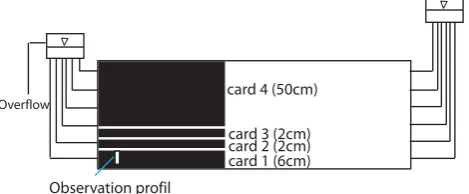
[image:6.595.325.528.97.187.2] [image:6.595.49.286.338.545.2]card 1 (6cm) card 2 (2cm) card 3 (2cm) card 4 (50cm)
[image:7.595.309.546.63.175.2]Observation profil Overflow
Fig. 6. Setup of the experiment E1. The cards are placed one after another right above each other, the heights of the cards are written in brackets.
high enough so that, even with a large dilution, e.g. 0.5 g/l salt (corresponding to 0.005 g/l color), the plume can be dif-ferentiated optically from the ambient pore water. However, the maximum concentration needs to be below intensity sat-uration to enable the correct resolution of the high concen-trations.
The parameters of the calibration curve had to be derived for each specific observation point (Table 2). Thus, back-ground levelling, as suggested in Schincariol et al. (1993) to compensate the spatially uneven lighting in the tank, was not necessary. This is an advantage because background level-ling can reduce the dynamic range and adds noise to the orig-inal data (Russ, 1999). Once the parameters of the standard curve are determined, they apply to all experiments if illumi-nation and camera position is constant. This approach offers a computationally effective way to derive the high-resolution time series of concentrations.
3.5 Impact of lens flare on measured intensities
The basis of photometry in terms of concentration measure-ments of fluids is as follows: the brightness of two solutions is of equal intensity during calibration and all stages of the experiment, provided that the solutions are equally concen-trated (Arnold et al., 1971). However, this prerequisite could become perturbed due to the effects of lens flare. Rogers (in Newman, 1976) stated: “one of the most usual prob-lems created by white backgrounds is that of flare, caused by excessive reflection from white surface into the camera lens [. . . ].” In porous media experiments, the artificial glass beads cause high reflection intensity and might generate flare effects, which have enough intensity to perturb the measure-ments. Regions of the photographed domain, which have a high dye concentration, might appear brighter because of the lens flare effects. That causes an underestimation of concen-trations. We conducted a series of experiments in order to investigate the impact of lens flare effects on reflected inten-sity measurements (Table 1).
In experiment E1, we successively placed four 70 cm long black cards one after another at the left side of the front win-dow of our tank as illustrated in Fig. 6. Fifty images were
Distance to upper edge of first card (cm)
0-0.5 0.5-1.0 1.0-1.5 1.5-2.0 2.0-2.5 2.5-3.0 3.0-3.5
Dev
iation (
%
)
0 2 4 6 8 10
[image:7.595.51.286.66.163.2]Deviation 1st setup to 2nd setup Deviation 1st setup to 3rd setup Deviation 1st setup to 4th setup
Fig. 7. Deviation (decline) of intensities taken at the profile in Fig. 6 when adding cards above card 1.
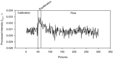
made of each of the 4 steps. Figure 7 shows the decline of intensities along a vertical profile on card 1 (Fig. 6) for the four steps of the experiment. Adding cards 2 to 4 above card 1 decreases the reflection from the porous media above card 1 and therefore the effect of flare was reduced and made card 1 appear darker. The fourth stage of E1 is comparable to the calibration phase of E2 (see Sect. 3.4) when the entire tank was filled with the dyed saltwater and lens flare significantly reduced. However, the dye tracer did not affect the largest portion of the tank during the flow phase of E2, and reflec-tion intensity of the porous media was high. The shape of the salt body during the upconing process of the flow phase of E2 is shown schematically in Fig. 1. Flare effects like in E1 can occur. In order to demonstrate the flare effects in E2 we derived intensities at a point 2 cm above the ground. The po-sition of this measurement point is equal to the observation hole P1 of E3 (Fig. 2). Concentration profiles showed that the transition zone of the saltwater at the end of the equili-bration phase, the second phase of the saltpool experiment, started 3 cm above the ground. Therefore, the concentration is necessarily 100 g/l at 2 cm above ground. Since the salt body moves upwards to the outlet during the course of the experiment, no concentration changes are expected at this point. The intensities in Fig. 8 show a clear shift from 100 g/l calibration to the equilibration phase (approximately 7% in-crease in intensity) and from calibration to the flow phase (approximately 3%). The intensity values decline during the upconing process of the flow phase. With the upconing of the saltwater, the dyed water affects a larger region around the observation point and reflection intensities are reduced. Therefore, the flare effects are reduced and the deviation be-tween calibration intensities for 100 g/l and the measured in-tensities during the flow phase decline to 3%. This effect is comparable to the effects observed in E1 when the black cards are attached above card 1.
Pictures
0 50 100 150 200 250 300 350 400 450 500
Pr
oc
es
sed inten
sity
(
Icorr
,
-)
0.018 0.019 0.020 0.021 0.022 0.023
[image:8.595.49.285.63.170.2]Calibration Equilibration Flow
Fig. 8. Intensities of P1 (without mask) where no concentration changes occur during the flow phase of the density flow experiment (constant concentration of 100 g/l).
Pictures
0 50 100 150 200 250 300 350
Pr
oc
es
se
d intens
ity
(
Icorr
,
-)
0.028 0.029 0.030 0.031 0.032 0.033 0.034
Calibration
Equil
ibratio
n
[image:8.595.310.547.63.106.2]Flow
Fig. 9. Intensities of observation point P1 with mask.
points where we wanted to derive breakthrough curves for the third experiment E3 (Fig. 2). The upconing took place at the left side of the domain below the outlet. Therefore, as many observation points as possible were distributed in or close to the area of the expected saltwater upconing. Fig-ure 9 shows the intensities of P1 during all stages of the ex-periment. It becomes evident that the effect of lens flare is strongly reduced, especially during the flow phase (0% in-tensity deviation between calibration and flow phase). How-ever, there is still an approximately 3% deviation between the intensities of the calibration and the equilibration phases of E3. We attribute this effect to the impact of the observa-tion points close to P1. These were not influenced by the dye and therefore reflection intensity was high and, hence, could cause lens flare effects. During the course of the experiment the salt plume rose and the points in the neighbourhood of P1 appeared darker, which reduced flare effects during the flow phase comparable to the effects observed in E1 and E2. Therefore, the attached mask helps to reduce flare effects.
[image:8.595.49.285.234.357.2]The experiment E4 was conducted to estimate the error caused by flare effects. Solutions of predetermined 5, 40, and 100 g/l (salt+dye) were progressively pumped into the tank from the bottom upward. Seven different filling levels with a horizontally planar salt water front were established so that all observation points in the same horizontal line were fully immerged in the solution. In order to estimate the impact
Fig. 10. Mass balance analysis of E5 after 10 min and 45 min.
of lens flare we derived intensities at all observation points visible in Fig. 2 (not only P1–P4) for all filling levels of the experiment of the three solutions and analyzed their develop-ment during the course of the experidevelop-ment. E4 revealed that the error depends on (i) the concentration of the solution, and the error increases with increasing concentration; and (ii) the intensity of the neighboring observation points, while the er-ror decreases with decreasing intensity. The maximal devi-ation of intensities for the 100 g/l solution in E4 amounted to 3%. This experiment shows only 1-D vertical movement of the brine, and 2-D plume shapes such as in the saltpool experiments E2 and E3 do not occur. Therefore, we used the results of E4 only to estimate the error caused by lens flare effects, and not to correct the measured data. We assumed a maximal error of 3% of overestimation (compared to calibra-tion) of the intensities during the flow phase caused by lens flare effects for E3 with the attached mask.
3.6 Error assessment
In order to estimate the precision of the photometric method, we calculated the standard deviation of the calibration im-ages for each calibration step (Fig. 5A). The maximum de-viation, which we consider as the accuracy of the measured intensities, occurs for salt concentration of calibration steps 70 g/l or 100 g/l. From the above discussion, we know that there is an additional error of +3% in the measured intensities due to the lens flare effect. Therefore, the concentrations are given with confident limits (see Fig. 16). The lower boundary is calculated from the processed intensityIcorrplus standard
deviation (%), whereas for the upper boundaryIcorr minus
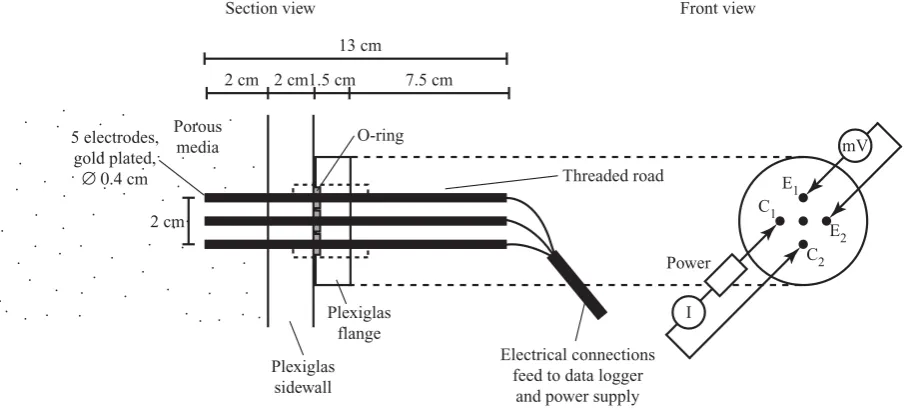
5 electrodes, gold plated,
∅ 0.4 cm
Section view
O-ring 13 cm
2 cm
2 cm 2 cm1.5 cm 7.5 cm
Front view
Electrical connections feed to data logger
and power supply Porous
media
Threaded road
Power
E1
C2
C1
E2
I
mV
Plexiglas flange
[image:9.595.71.526.66.271.2]Plexiglas sidewall
Fig. 11. Electrode array with two current electrodes (C1and C2), two potential electrodes (E1and E2)and grounding in the center of the array.
images after 10 and 45 minutes. Figure 10 shows the spatial distribution of the saltwater (red). The 10 min image deliv-ers an underestimation of the total mass of –4.2% compared to the mass entering the domain. This is within the range of expected lens flare error. After 45 min, the bright region of the tank is significantly reduced and the mass error accounts for 1.6% indicating that the method overestimates the total mass. On the basis of this analysis, the calibration parame-ters of Eq. 4 can be considered reliable, and possible errors can be explained by the impact of lens flare.
4 Concentration determination with resistivity
measur-ing cells (RMC)
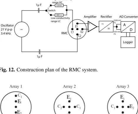
4.1 Technical setup of the RMC system
Each RMC consists of five gilded stainless steel electrodes (diameter 0.4 cm, length 13 cm, Fig. 11). We used gilded electrodes, because uncontrollable fluctuations in the resis-tivity measurement occur with ungilded stainless steel elec-trodes. The electrodes are equally spaced 1 cm around the center electrode and mounted on a Plexiglas flange. They are installed perpendicular to the flow direction through the back wall of the tank. Figure 12 shows the schematic con-struction plan of the entire RMC system. The system in-volves measuring the output voltage between the electrodes E1and E2while electrical current is caused to flow through
the porous media between the outer pair of electrodes C1and
C2. The grounding electrode is in the center. The
measur-ing principle is based on a 4-electrode resitivity measurement technique, where the current is supplied through a very pre-cisely regulated sinusoidal oscillator signal. The measured
AC voltage is rectified through a synchronous demodulator in phase to the oscillator. The resulting DC output voltage was recorded utilizing a micro-logger and a relais based mul-tiplexer to measure all the RMCs sequentially. An alternating current was applied in all measurements to minimize polar-ization within the cell and to prevent movement of the ions due to the presence of a voltage potential.
Since the measurement has to cover a wide range of volt-age values due to the high salt concentrations, two differ-ent input voltages are used at each time step. This enables measurements to be made in two measurement ranges, one for the high concentration, referred to as MR1, and the other for low concentrations, MR2. As this measuring method is sensitive to temperature variations, temperature sensors (YSI 4006; accuracy±0.01◦C) are also inserted into the porous medium.
4.2 Electrode arrays
Various electrode arrays were tested in preliminary experi-ments in a small container (35×16×9 cm3)filled with satu-rated porous media. Figure 13 shows the three investigated arrays. In array 1 all electrodes are uniformly placed in a line with the grounding electrode in the center. Array 2 is a cross-placement of C1,2(current electrodes) and E1,2
C1 C2 E1 E2 + - = ~ ~ D A 2500 mV FS 250 mV FS Logger Amplifier Rectifier AD Converter
Oscillator 21 V p-p 3.4 kHz 1µ F 1µ F High conductivity range HC Low conductivity range LC
6.8 kW
680 W
RMC
[image:10.595.50.287.63.166.2]Switch
[image:10.595.49.284.67.261.2]Fig. 12. Construction plan of the RMC system.
Fig. 13. Evaluated sets of electrode arrays.
front in the small experimental tank. Figure 14 shows the measured breakthrough curves of output voltages of the 8 different arrangements.
The breakthrough curves of array 1 and its clockwise ro-tated (by 90◦) setup clearly show the dependence of these alignments on the flow direction of the salt front. There is a temporal shift between both curves, and array 1 even shows a plateau of the curve. Array 2 delivers no analyzable break-through curve. In this setup, both electrodes should detect the same voltage under homogeneous conditions. The fact that a voltage change is visible might be due to local concentration differences or asymmetric manufacturing of the RMC. Array 3 and its rotated setups deliver curves less dependent on the flow direction of the front and a realistic shape of the curve is observed. As the result of these findings, we chose array 3 for measuring the resistivity.
4.3 Calibration of the RMC
The resistivity measured between two electrodes is a function of the porous material, porosity, temperature, geometrical ar-rangement of the electrodes, state of gold coating and the ion concentration (Telford et al., 1990). During an experiment, all factors apart from the ion concentration are kept constant and the measured resistivity can be related to the concentra-tion of the soluconcentra-tion surrounding the electrodes. This rela-tionship has to be determined via calibration experiments as described in Sect. 3.4. The output voltages of the two mea-suring ranges, MR1 and 2, are correlated with the concentra-tions using specifically fitted power laws for each RMC and measurement range. Figure 15 shows, by way of example, the calibration curves for MR1 and 2 of the RMC located at observation point P2 (Fig. 2).
Ou tp ut voltag e (m V) 0 200 400 600 800 1000 1200 1400 1600
Array 1 rotated clockwise by 90° Array 1 Ou tp ut v ol tag e (m V) -1000 -5000 500 1000 1500 2000 2500 3000 Array 3 rotated clockwise by 90° Array 2 Output v oltage (m V) 0 500 1000 1500 2000 2500 Array 3
Array 3 rotated clockwise by 180°
Brine inflow (min)
0 10 20 30 40 50 60 70 80 90 100 110 120 130 140 Output
v oltage (m V) 0 500 1000 1500 2000 2500 3000 Array 3
Array 3 rotated clockwise by 315° Array 3 rotated clockwise by 135°
Fig. 14. Measured breakthrough curves of output voltage (mV) for the different sets of electrodes and their clockwise-rotated arrange-ments.
Output voltage (mV)
0 50 100 150 200 250 300 350 400
Co nc en tr ation ( g/l) 0 20 40 60 80 100 120
Fitted curve for MR2 Fitted curve for MR1 Measurments MR1 Measurments MR2
Equation: C=A*V^B
C: Concentration (g/l) A, B: Fitting parameters V: Output voltage (mV)
R2
MR1=0.999
R2
MR2=0.999
AMR1 16808.93 +/- 1894.35
AMR2 756.92 +/- 76.56
BMR1 -1.3021 +/- 0.027
BMR2 -1.2171 +/- 0.027
Fig. 15. Calibration curves for the RMC at P2.
The errors associated with the concentration consist of two parts: measurement errors and parameter errors associated with the calibration curves. The measurement errors are small and the maximum error found during the calibration experiment was +/–0.5%. The errors associated with the cali-bration curve are within the range of –1.5 to +2.5%. Since the calculated error is small we do not show error bars in Fig. 16. Typically, systematic errors are caused by temperature fluc-tuations. However, these can be minimized for laboratory experiments due to controlled room and water temperatures.
5 Comparison of the two methods
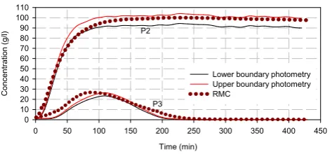
[image:10.595.311.545.67.231.2] [image:10.595.309.544.293.463.2]both independent methods reproduce the expected concentra-tions of 100 g/l at P2 when the saltwater rises, although the RMC shows a slightly earlier reaction than the image analy-sis approach, which can be explained by the larger measure-ment volume of the RMC (Fig. 16).
However, if the electrode is placed within the transition zone, where steep concentration gradients exist, the two methods differ significantly due to the different measurement volumes, as is the case at P3 (Fig. 16). The RMC measures an apparent resistivity of the environment around the elec-trodes. Thus, it is not a point measurement but an integral value. The measurement volume strongly depends on the ion concentration distribution and on the resistivity contrast dur-ing the experiment. Therefore, the measurement volume is not constant throughout the course of the experiment. This problem is the major drawback of the RMC method espe-cially for measuring points within the transition zone, where a concentration gradient occurs within the measuring volume of the RMC. However, especially for points such as P2 where the electrodes are surrounded by a uniform concentration, this problem is of minor importance. A numerical simulation of the resistivity field, the current density and of the voltage at the electrodes for heterogeneous resistivity distributions could enable the determination of the measurement volume. This work was beyond the scope of this study but we highly recommend further investigation in this field.
6 Conclusions
In this study we present a photometric methodology, which enables effective computation of high-resolution time series of plume concentrations. The method is capable of treat-ing a large number of images since only one optimization of the intensity vs. concentration standard curve is required. Once the parameters of this curve are known for the obser-vation point they can be used for a series of experiments, if the camera position and the tank position do not change and the images fit on a pixel-by-pixel basis. Beside the break-through curves contour lines of concentration can be deter-mined. The resolution of the observation point is crucial for the precision of the measured intensity values. Therefore, we suggest a statistical analysis for each experimental setup to determine the adequate resolution. A major source of error is the impact of lens flare. High reflections of bright regions of the photographed domain, which are not influenced by the dye, could generate flare effects that increase the measured intensity of dark, dye-influenced regions of the tank. This leads to an underestimation of the concentration. Attaching a mask at the front window of the tank, which reduces the percentage of bright regions, can minimize this effect. How-ever, information is available in this case only at the predeter-mined points, i.e., the observation holes in the mask. Since the mask itself influences the brightness of the observation holes, both the calibration and the flow experiments have to
Time (min)
0 50 100 150 200 250 300 350 400 450
Co
nc
en
tr
ation
(
g/l)
0 10 20 30 40 50 60 70 80 90 100 110
Lower boundary photometry Upper boundary photometry RMC
P2
[image:11.595.311.548.62.172.2]P3
Fig. 16. Breakthrough curves of P2 (100 g/l) and P3 (max. 30 g/l) derived from electrodes and from photometric method. The solid lines represent the range of error of the photometric method.
be conducted using the same setup with the mask. This min-imizes the flexibility of the experiment in order to run dif-ferent experiments with changing boundary conditions and therefore with different plume patterns.
Nevertheless, the precision of the measurement is high even without the mask. A successive filling of the tank with predetermined concentrations of salt-dye solutions enables an estimation of the error caused by flare effects. The suc-cessive filling gradually reduced the percentage of bright re-gions and therefore decreased the impact of flare effects at the observation points. The deviation between the measured intensity of the entirely filled tank and the partly filled tank was determined as maximal error.
In this study, the light reflection technique was used in-stead of the transmission technique because:
1. The back of the tank holds devices to measure resistiv-ity, temperature and pressure;
2. Applicability and limitations of the widely used reflec-tion method need to be assessed.
For future research, we suggest a direct comparison of the light reflection and the transmission techniques.
points within the tank. A numerical analysis of the measure-ment volume of the RMC system could help to improve the applicability of the technique for detailed laboratory-scale flow experiments. Regarding hydrogeological field observa-tions, the RMC method could be further developed for multi-level monitoring of electrical conductivities in the context of highly saline groundwaters mixing with groundwaters of low salinity. This is of special interest in active evaporite subro-sion and/or forced groundwater circulation systems (active pumping). Resistivity tomography could be tested and com-pared with the imaging method – viewing the results of the imaging method as “true” system behaviour.
Acknowledgements. The authors are grateful to Claude Veit (IMFS, Strasbourg) who constructed the Plexiglas flow tank and to Prof. Wieland for support during the development of the RMC method. Lukas Rosenthaler of the Imaging and Media Lab, University of Basel contributed significantly to the image analysis method. We acknowledge the valuable comments of two anonymous referees
and of the editor. This study was financed by the Schweizer
Nationalfond 200020-109200.
Edited by: C. Hinz
References
Arnold, C., Rolls, P., and Stewart, J.: Applied photography, The Focal Press, ISBN 0-240-50723-1, 1971.
Barth, G. R., Illangesekare, T. H., Hill, M. C., and Rajaram, H.: A new tracer-density criterion for heterogeneous porous media, Water Resour. Res., 37, 21–31, 2001.
Catania, F., Massabo, M., Valle, M., Bracco , G., and Paladino, O.: Assessment of quantitative imaging of contaminant distributions in porous media, Exp Fluids 44, 167–177, 2008.
Corapcioglu, M. Y., Chowdhury, S., and Roosevelt, S. E.: Mi-cromodel visualization and quantification of solute transport in porous media, Water Resour. Res. 33, 11, 2547–2558, 1997. Danquigny, C. Ackerer, P., and Carlier, J. P.: Laboratory tracer tests
on three-dimensional reconstructed heterogeneous porous media, J. Hydrol., 294(1-3), 196–212 Sp. Iss. SI JUL 15, 2004. Detwiler, R. L., Rajaram, H., and Glass, R. J.: Solute transport in
variable-aperture fractures: An investigation of the relative im-portance of Taylor dispersion and macrodispersion, Water Re-sour. Res. 36, 7, 1611–1625, 2000.
Goswami, R. and Clement, P.: Laboratory-scale investigation of saltwater intrusion dynamics, Water Resour. Res., 43, W04418, doi:10.1029/2006WR005151, 2007.
Hassanizadeh, S. M. and Leijnse, A.: A non-linear theory of high-concentration-gradient dispersion in porous media, Advances in Water Resour., 18(4), 203–215, 1995.
Huang, W., Smith, C. C., Lerner, D. N,. Thornton, S. F., and Oram A.: Physical modelling of solute transport in porous media: eval-uation of an imaging technique using UV excited fluorescent dye., Water Res 3(7), 1843–1853, 2002.
Jones, E. H. and Smith, C. C.: Non-equilibrium partitioning tracer transport in porous media: 2-D physical modelling and imaging using a partitioning fluorescent dye, Water Res 39(2)0, 5099– 5111, 2005.
McNeil, J. D., Oldenborger, G. A., and Schincariol, R. A.: Quan-titative imaging of contaminant distributions in heterogeneous porous media laboratory experiments. J. Contam. Hydrol., 84, 36–54, 2006.
Oostrom, M., Dane, J. H., Guven, O., and Hayworth, J. S.: Ex-perimental investigation of dense solute plumes in an unconfined aquifer model, Water Resour. Res., 28, 2315–2326, 1992. Oostrom, M., Hofstee, C., Lenhard, R. J., Wietsma, and T. W.: Flow
behavior and residual saturation formation of liquid carbon tetra-chloride in unsaturated heterogeneous porous media, J. Contam. Hydrol., 64, 93–112, 2003.
Oswald, S., Kinzelbach, W., Greiner, A., and Brix, G.: Observa-tion of flow and transport processes in artificial porous media via magnetic resonance imaging in three dimensions, Geoderma 80, 417–429, 1997.
Oswald, S. and Kinzelbach, W.: Three-dimensional physical bench-mark experiments to test variable-density flow models, J. Hy-drol., 290, 22–42, 2004.
Rahman, A., Jose, S., Nowak, W., and Cirpka, O.: Experiments on vertical transverse mixing in a large-scale heterogeneous model aquifer, J. Contam. Hydrol., 80, 130–148, 2005.
Rogers, G.: Photography in paediatrics, Published in photographic techniques in scientific research, Volume 2, edited by Newman, A., Academic Press, ISBN 0 12 517960, 1976.
Russ, J. C.: The image processing handbook, 3rd edn. CRC, Boca Raton, 1999.
Schincariol, R. A., Herderick, E. E., and Schwartz, F. W.: On the application of image analysis to determine concentration distri-butions in laboratory experiments, J. Contam. Hydrol., 12, 197– 215, 1993.
Silliman, S. E., Zheng, L., and Conwell, P.: The use of laboratory experiments for the study of conservative solute transport in het-erogeneous porous media, Hydrogeol. J., 6, 166–177, 1998. Simmons, C. T., Pierini, M. L., and Hutson, J. L.: Laboratory
investigation of variable-density flow and solute transport in unsaturated–saturated porous media, Transp. Porous Media 47, 15–244, 2002.
Swartz, C. H. and Schwartz, F. W.: An experimental study of mix-ing and instability development in variable-density systems, J. Contam. Hydrol., 34, 169–189, 1998.
Telford, W. M., Geldart, L. P., and Sheriff, R. E.: Applied geo-physics, – 2nd edition, Cambridge University Press, ISBN 0-521-33938-3, 1990.
Theodoropoulou, M. A., Karoutsos, V., Kaspiris, C., and Tsakiroglou, C. D.: A new visualization technique for the study of solute dispersion in model porous media, J. Hydrol., 27(1–4), 176–197, 2003.