Minimization of Portfolio Risk using Three Different
Methods (A Comparative Study)
Hegazy Zaher
Professor of Mathematical Statistics, Institute of Statistical Studies and Research (ISSR),
Cairo University, Egypt
Nisren Hassanen Mohamed
Ph.D. student, Dept of Operations Research Institute of Statistical Studies and Research
(ISSR), Cairo University, Egypt
ABSTRACT
Portfolio risk plays an important role in stock market decisions. This paper considers an alternative idea which is to compute the risk assuming fixed return. Three different methods used to study this problem. The given study suggests expressing the general index of a given stock market in terms of other countries stock markets. A comparison between the three proposed methods is conducted using three different measures of error (the Mean-Variance (MV), Mean-Absolute Deviation (MAD), Conditional Value-at-Risk (CVaR)). The obtained results show that there are significant differences between the used methods. It is recommended using the simplest one.
Keywords
Portfolio Risk, Risk Minimization, Stock Market Indicators, Absolute Deviation, Conditional Value-At-Risk, Mean-Variance, Return Maximization
1.
INTRODUCTION
Risk is one of the important factors in portfolio optimization problem [1]. Many studies have proposed alternative risk measures to overcome the drawbacks of variance. Individuals are trying to allocate their capitals to select the suitable securities in order to reach the investment goals. The first mathematical model considering both measures (minimize the risk and maximize the return) given by Markowitz [2, 3]. Konno and Yamazaki [4] introduced a linear optimization model for the given problem. In particular, when the returns of the portfolio are multivariate normally distributed, the model is equivalent to Markowitz's mean-variance model [5]. Based on absolute deviation, many models were developed such as [6, 7, and 8].The basic idea of this paper is to investigate the effect of changes in the global stock market indicator expressed in terms of other countries stock market indicators. The basic target is to increase the investor’s future confidence in stock markets decisions. This paper also finds the effect of changes in the foreign stock markets indicators on the local stock markets indicator as given by authors in [9]. The used data is the historical data of Gulf Area Stock Markets, (Bahrain Stock Exchange (BSE), Doha Securities Market (DSM), Abu Dhabi Securities Exchange (ADSM), Kuwait Stock Exchange (KSE), Muscat Securities Market (MSM), Dubai financial market (DFM), local stock markets, (Cairo & Alexandria Stock Exchange (CASE 30)). Moreover, International Stock Markets, (Brazil, Mexico, India, Malaysia, Canada, Switzerland (SWISS),United States of America (USA), United Kingdom (UK), South Korea, Indonesia, Norway, Singapore, Japan, Hong Kong, Germany, France, Australia. The used data in this study considers the time interval from December 21, 2005 to July 15, 2008 [9].
This work is based on two basic steps:
1- To select the most important indicators affecting the stock market indicator under consideration [9].
2- To use the selected indicators to attain the required objectives (min risk at certain return level).
The inputs will be indicators of the other countries, and the output will be the indicator of the country under consideration. MV, MAD, and CVaR techniques will be used to model the problem under consideration.
The General stock market Index can be computed using the following formula:
1
1
( ) ( ( )
(
)) / (
)
i
n
i
n
i
n
i
n
R t
P t
P t
P t
(1)For each asset, the expected returnfor n assets is estimated by
1(
)
n
P i i
i
E r
w E r
(2)
Where
:
n = the number of securities;
i
w
= he proportion of the funds investedin security i.
,
i P
r r
= the return on ith security andportfolio p.
E
=the expectation of the variable in the parentheses.
Pi = price of the ith security
and portfolio p.
Assuming the portfolio has N assets with returns Ri, i= 1... N.
2.
RISK MEASURES
2.1
Mean Variance (MV)
(3)
(4)
(5)
Where,
Ri= Return on asset i
Wi = Weight of component asset i (that is, the share of the asset i in the portfolio).
Wj = Weight of component asset j (that is, the share of the asset j in the portfolio).
ρij = correlation coefficient between the rates of return on
security i, ri , and the rates of return on security j, rj
i
= standard deviations of r
i.
j
= standard deviations of rj.
n = the number of securities. E = the target expected return.
The first constraint (4) refers to that the expected return on the portfolio should equal to the target return determined by a portfolio manager. The second constraint (5) indicates that the weights of the securities invested in the portfolio must sum to one [12]-[13]-[14].
2.2
Mean Absolute Deviation (MAD)
Konno and Yamazaki [4] use a linear programming model for portfolio optimization in which the risk measure is the mean absolute deviation (MAD). This model calculates the portfolio to minimizing MAD subject to a lower bound on the return. The model can be expressed by the following equation [4]:
1
1
min
|
(
( )
) |
i
N
w i i n i
n i s
w
R t
R
N
(6)
3.
CONDITIONAL VALUE-AT-RISK
(CVAR)
A risk minimization technique often used to reduce the probability that the portfolio will incur large losses. CVaR, also called Mean Excess Loss, Mean Shortfall or Tail VaR, presented by Rockafellar and Uryasev [15] introduced the notion of the expected loss when exceeding Value-at-Risk (VaR) [16]. The model can be expressed by the following equations [17, 18]:
The conditional value-at-risk for a portfolio , is defined a
( , ) ( )
1
( )
( , ) ( )
1
f x y VaR xCVaR x
f x y p y dy
(7)
Where:
α = the probability level such that 0 < α < 1.
f(x,y) = the loss function for a portfolio x and asset return y.
p(y) = the probability density function for asset return y.
VaRα = the value-at-risk of portfolio x at probability level α.
The value-at-risk is defined as
An alternative formulation for CVaR has the form:
1
( )
( )
max 0, ( ( , )
( )) ( )
1
rCVaR x
VaR x
f x y
VaR x
p y dy
(8)
The choice for the probability level α is exactly 0.9 or 0.95.
3.1
Models Experimentation
The Experimental data are gathered directly from daily stock market indices for a period of 663 days starting on December 21, 2005 till July 15, 2008. The following stock markets were included in this study with their global indicators: Cairo & Alexandria Stock Exchange (CASE 30), Bahrain Stock Exchange (BSE), Doha Securities Market (DSM), Dubai Financial Market (DFM), Kuwait Stock Exchange (KSE), Muscat Securities Market (MSM), USA, France (CAC40), United Kingdom (FTSE100), Norway, India, Hong Kong, Japan, Switzerland (SWISS), Singapore, and Canada. Second the following algorithm is used to generate solutions satisfying the model given in (3).
3.2
Solution Algorithm of:
Model 1 (MV) [2, 3]
Step 1
Find the mean, standard deviations and the variance of similar indices in other stock markets. Also find the Correlation coefficient and the Covariance [19, 20].
Step 2
Start with any portfolio weights.
Step3
Use equations (1), (2) and (3) from the previous section to compute the portfolio general stock market index, means variance and standard deviation.
Step 4
Calculate the minimum variance portfolio from (3).
Step5
2
1
1
subject to
(R )
1
1.0
1
n
n
Min
X
w w
i
j ij i
j
i
j
n
w E
I
E
i
i
n
w
i
i
Set the maximum satisfying minimum variance and specify the constraints as in equations (4) and (5). Select the range of the portfolio weights of the risky assets to reach the optimization solution. The solution is shown in tables 1, 2,3,4,5,6. Where the optimal portfolio risks (as measured by the standard deviation) and the corresponding portfolio expected monthly return. The weights in the optimal portfolio are also shown in Tables 1, 2,3,4,5,6 for each (16) countries.
Model 2 [MAD] [4]
Step 1
Find the mean, standard deviations and the variance of similar indices in other stock markets. Also find the Correlation coefficient and the Covariance.
Step 2
Start with any portfolio weights.
Step3
Calculate the minimum variance portfolio from (6) under the same constraints as in equations (4) and (5).
Step 4
Select the range of the portfolio weights of the risky assets to reach the optimization solution. The solution is shown in tables 1, 2,3,4,5,6. Where the optimal portfolio risks (as measured by the standard deviation) and the corresponding portfolio expected monthly return. The weights in the optimal portfolio are also shown in Tables 1, 2,3,4,5,6 for each (16) countries.
Model 3 (CVaR) [15, 16]
Step 1
Find the mean, standard deviations and the variance of similar indices in other stock markets. Also find the Correlation coefficient and the Covariance [21].
Step 2
Start with any portfolio weights. Step3
Calculate the minimum variance portfolio from (7) under the same constraints as in equations (4) and (5).
Step 4
Select the range of the portfolio weights of the risky assets to reach the optimization solution. The solution is shown in tables 1, 2,3,4,5,6. Where the optimal portfolio risks (as measured by the standard deviation) and the corresponding portfolio expected monthly return. The weights in the optimal portfolio are also shown in Tables 1, 2,3,4,5,6 for each (16) countries.
4.
EXPERMENTAL RESULTS
Table 1 portfolio risk with assuming fixed return
country
models MV MAD CVaR MV MAD CVaR 0.7051 (BSE) 0.7132 (BSE) 0.6954 (BSE) 0.5223 (BSE) 0.5224 (BSE) 0.5197 (BSE) 0.0282 (Brazil) 0.0283 (Brazil) 0.0265 (Brazil) 0.0002 (DSM) 0.0006 (DSM) 0.0011 (DSM) 0.0171 (CAC40) 0.0153 (CAC40) 0.0253 (CAC40) 0.2315 (KSE) 0.2363 (KSE) 0.2341 (KSE) 0.0847 (Mexico) 0.0809 (Mexico) 0.0885 (Mexico) 0.0166 (Singapore) 0.0149 (Singapore) 0.0160 (Singapore) 0.0069 (India) 0.0043 (India) 0.0065 (India) 0.1351 (Malaysia) 0.1323 (Malaysia) 0.1318 (Malaysia) 0.0195 (South Korea) 0.0181 (South Korea) 0.0157 (South Korea) 0.0171 (India) 0.0159 (India) 0.0193 (India) 0.0771 (Indonesia) 0.0782 (Indonesia) 0.0777 (Indonesia) 0.0242 (Indonesia) 0.0249 (Indonesia) 0.0266 (Indonesia) 0.0613 (China) 0.0616 (China) 0.0644 (China) 0.0530 (China) 0.0528 (China) 0.0513 (China) expected
return 0,0005 0,0005 0,0005 0,0005 0,0005 0,0005 portfolio
std.deviation 0,0049 0,0049 0,0049 0,0045 0,0045 0,0045 Singapore Hong Kong
Table 2 continue
country
models MV MAD CVaR MV MAD CVaR MV MAD CVaR 0.0553 (ADSM) 0.0550 (ADSM) 0.0557 (ADSM) 0.6000 (BSE) 0.6036 (BSE) 0.5951 (BSE) 0.7175 (BSE) 0.71499 (BSE) 0.7177 (BSE) 0.0686 (DSM) 0.0688 (DSM) 0.0658 (DSM) 0.0738 (CASE30) 0.0739 (CASE30) 0.0728 (CASE30) 0.0422 (DSM) 0.0440 (DSM) 0.0385 (DSM) 0.60100 (KSE) 0.6103 (KSE) 0.6116 (KSE) 0.2145 (KSE) 0.2106 (KSE) 0.2214 (KSE) 0.0556 (Brazil) 0.05602 (Brazil) 0.0568 (Brazil) 0.1695 (South Korea) 0.1695 (South Korea) 0.1712 (South Korea) 0.0878 (Norway) 0.0875 (Norway) 0.0884 (Norway) 0.1204 (SWISS) 0.1204 (SWISS) 0.1237 (SWISS) 0.0966 (China) 0.0965 (China) 0.0958 (China) 0.0239 (South Korea) 0.0243 (South Korea) 0.0223 (South Korea) 0.0642 (China) 0.0646 (China) 0.0634 (China) expected
return 0,0005 0,0005 0,0005 0,0004 0,0004 0,0004 0,0004 0,0004 0,0004 portfolio
std.deviation 0,0064 0,0064 0,0064 0,0046 0,0046 0,0046 0,0049 0,0049 0,0049 Norway United Kingdom United States of America
Table 3 continue
country
models MV MAD CVaR MV MAD CVaR MV MAD CVaR
0.0474 (ADSM) 0.0475 (ADSM) 0.0482 (ADSM) 0.1917 (ADSM) 0.1893 (ADSM) 0.192 (ADSM) 0.0257 (DSM) 0.0264 (DSM) 0.0262 (DSM) 0.0280 (DSM) 0.0314 (DSM) 0.0319 (DSM) 0.1177 (CASE30) 0.1152 (CASE30) 0.1176 (CASE30) 0.3608 (MSM) 0.3631 (MSM) 0.3606 (MSM) 0.0574 (CASE30) 0.0622 (CASE30) 0.0529 (CASE30) 0.4079 (Canada) 0.4074 (Canada) 0.4150 (Canada) 0.3623 (KSE) 0.3574 (KSE) 0.3625 (KSE) 0.4981 (KSE) 0.4924 (KSE) 0.5017 (KSE) 0.0129 (Norway) 0.0166 (Norway) 0.0110 (Norway) 0.0155 (Brazil) 0.0156 (Brazil) 0.0145 (Brazil) 0.2509 (Malaysia) 0.2489 (Malaysia) 0.2414 (Malaysia) 0.0702 (Japan) 0.0717 (Japan) 0.0690 (Japan) 0.1017 (Mexico) 0.0984 (Mexico) 0.1038 (Mexico) 0.0476 (SWISS) 0.0473 (SWISS) 0.0542 (SWISS) 0.1676 (SWISS) 0.1691 (SWISS) 0.1575 (SWISS) 0.0676 (Norway) 0.0676 (Norway) 0.0678 (Norway) 0.0706 (China) 0.0702 (China) 0.0698 (China) 0.0320 (Tasi) 0.0306 (Tasi) 0.0379 (Tasi) 0.0663 (South Korea) 0.0715 (South Korea) 0.0646 (South Korea) expected
return 0,0005 0,0005 0,0005 0,00020 0,00020 0,00020 0,0008 0,0008 0,0008 portfolio
std.deviation
0,0059 0,0059 0,0059 0,007 0,007 0,007 0,0053 0,0053 0,0053
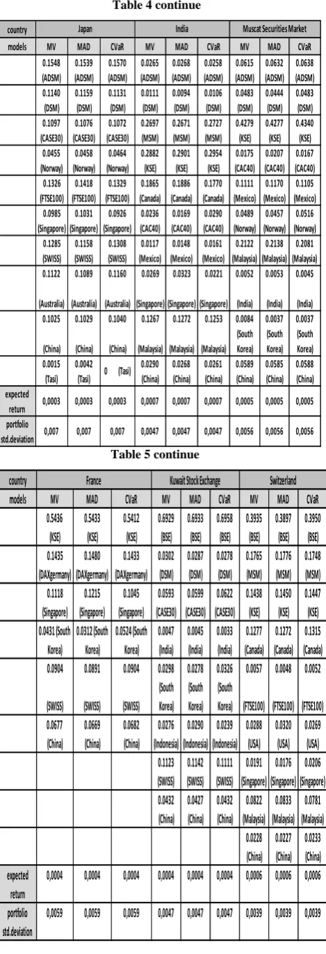
Table 4 continue
country
models MV MAD CVaR MV MAD CVaR MV MAD CVaR
0.1548 (ADSM) 0.1539 (ADSM) 0.1570 (ADSM) 0.0265 (ADSM) 0.0268 (ADSM) 0.0258 (ADSM) 0.0615 (ADSM) 0.0632 (ADSM) 0.0638 (ADSM) 0.1140 (DSM) 0.1159 (DSM) 0.1131 (DSM) 0.0111 (DSM) 0.0094 (DSM) 0.0106 (DSM) 0.0483 (DSM) 0.0444 (DSM) 0.0483 (DSM) 0.1097 (CASE30) 0.1076 (CASE30) 0.1072 (CASE30) 0.2697 (MSM) 0.2671 (MSM) 0.2727 (MSM) 0.4279 (KSE) 0.4277 (KSE) 0.4340 (KSE) 0.0455 (Norway) 0.0458 (Norway) 0.0464 (Norway) 0.2882 (KSE) 0.2901 (KSE) 0.2954 (KSE) 0.0175 (CAC40) 0.0207 (CAC40) 0.0167 (CAC40) 0.1326 (FTSE100) 0.1418 (FTSE100) 0.1329 (FTSE100) 0.1865 (Canada) 0.1886 (Canada) 0.1770 (Canada) 0.1111 (Mexico) 0.1170 (Mexico) 0.1105 (Mexico) 0.0985 (Singapore) 0.1031 (Singapore) 0.0926 (Singapore) 0.0236 (CAC40) 0.0169 (CAC40) 0.0290 (CAC40) 0.0489 (Norway) 0.0457 (Norway) 0.0516 (Norway) 0.1285 (SWISS) 0.1158 (SWISS) 0.1308 (SWISS) 0.0117 (Mexico) 0.0148 (Mexico) 0.0161 (Mexico) 0.2122 (Malaysia) 0.2138 (Malaysia) 0.2081 (Malaysia) 0.1122 (Australia) 0.1089 (Australia) 0.1160 (Australia) 0.0269 (Singapore) 0.0323 (Singapore) 0.0221 (Singapore) 0.0052 (India) 0.0053 (India) 0.0045 (India) 0.1025 (China) 0.1029 (China) 0.1040 (China) 0.1267 (Malaysia) 0.1272 (Malaysia) 0.1253 (Malaysia) 0.0084 (South Korea) 0.0037 (South Korea) 0.0037 (South Korea) 0.0015 (Tasi) 0.0042
(Tasi) 0 (Tasi) 0.0290 (China) 0.0268 (China) 0.0261 (China) 0.0589 (China) 0.0585 (China) 0.0588 (China) expected
return 0,0003 0,0003 0,0003 0,0007 0,0007 0,0007 0,0005 0,0005 0,0005
portfolio
std.deviation 0,007 0,007 0,007 0,0047 0,0047 0,0047 0,0056 0,0056 0,0056
[image:4.595.55.290.74.760.2]Japan India Muscat Securities Market
Table 5 continue
country
models MV MAD CVaR MV MAD CVaR MV MAD CVaR
0.5436 (KSE) 0.5433 (KSE) 0.5412 (KSE) 0.6929 (BSE) 0.6933 (BSE) 0.6958 (BSE) 0.3935 (BSE) 0.3897 (BSE) 0.3950 (BSE) 0.1435 (DAXgermany) 0.1480 (DAXgermany) 0.1433 (DAXgermany) 0.0302 (DSM) 0.0287 (DSM) 0.0278 (DSM) 0.1765 (MSM) 0.1776 (MSM) 0.1748 (MSM) 0.1118 (Singapore) 0.1215 (Singapore) 0.1045 (Singapore) 0.0593 (CASE30) 0.0599 (CASE30) 0.0622 (CASE30) 0.1438 (KSE) 0.1450 (KSE) 0.1447 (KSE) 0.0431 (South Korea) 0.0312 (South Korea) 0.0524 (South Korea) 0.0047 (India) 0.0045 (India) 0.0033 (India) 0.1277 (Canada) 0.1272 (Canada) 0.1315 (Canada) 0.0904 (SWISS) 0.0891 (SWISS) 0.0904 (SWISS) 0.0298 (South Korea) 0.0278 (South Korea) 0.0326 (South Korea) 0.0057 (FTSE100) 0.0048 (FTSE100) 0.0052 (FTSE100) 0.0677 (China) 0.0669 (China) 0.0682 (China) 0.0276 (Indonesia) 0.0290 (Indonesia) 0.0239 (Indonesia) 0.0288 (USA) 0.0320 (USA) 0.0269 (USA) 0.1123 (SWISS) 0.1142 (SWISS) 0.1111 (SWISS) 0.0191 (Singapore) 0.0176 (Singapore) 0.0206 (Singapore) 0.0432 (China) 0.0427 (China) 0.0432 (China) 0.0822 (Malaysia) 0.0833 (Malaysia) 0.0781 (Malaysia) 0.0228 (China) 0.0227 (China) 0.0233 (China) expected return
0,0004 0,0004 0,0004 0,0004 0,0004 0,0004 0,0006 0,0006 0,0006
portfolio std.deviation
0,0059 0,0059 0,0059 0,0047 0,0047 0,0047 0,0039 0,0039 0,0039 Switzerland France Kuwait Stock Exchange
Table 6 continue
country
models MV MAD CVaR MV MAD CVaR 0.0036 (ADSM) 0.0050 (ADSM) 0.0000 (ADSM) 0.0141 (ADSM) 0.0128 (ADSM) 0.0170 (ADSM) 0.4985 (BSE) 0.5006 (BSE) 0.5026 (BSE) 0.4998 (BSE) 0.5006 (BSE) 0.4999 (BSE) 0.0044 (DSM) 0.0000 (DSM) 0.0068 (DSM) 0.2027 (MSM) 0.2045 (MSM) 0.2020 (MSM) 0.2401 (MSM) 0.2419 (MSM) 0.2356 (MSM) 0.1262 (Canada) 0.1215 (Canada) 0.1257 (Canada) 0.1442 (Canada) 0.1446 (Canada) 0.1539 (Canada) 0.0264 (Norway) 0.0251 (Norway) 0.0310 (Norway) 0.0174 (Norway) 0.0147 (Norway) 0.0191 (Norway) 0.0271 (FTSE100) 0.0325 (FTSE100) 0.0182 (FTSE100) 0.0400 (Singapore) 0.0382 (Singapore) 0.0450 (Singapore) 0.0516 (USA) 0.0487 (USA) 0.0591 (USA) 0.0045 (Indonesia) 0.0051 (Indonesia) 0.0000 (Indonesia) 0.0009 (Japan) 0.0040 (Japan) 0.0000 (Japan) 0.0236 (SWISS) 0.0289 (SWISS) 0.0104 (SWISS) 0.0174 (Indonesia) 0.0143 (Indonesia) 0.0155 (Indonesia) 0.0237 (Australia) 0.0209 (Australia) 0.0266 (Australia) 0.0314 (China) 0.0338 (China) 0.0309 (China) 0.0024 (Tasi) 0.0023 (Tasi) 0.0006 (Tasi) expected return
0,0006 0,0006 0,0006 0,0006 0,0006 0,0006
portfolio std.deviation
0,004 0,004 0,004 0,0042 0,0042 0,0042 Dubai financial market Cairo & Alexandria Stock Exchange
5. DISCUSSION AND CONCLUSIONS
1- The notion of expressing the global indicator of any country in terms of the global indicators of other countries introduced in [9] is correct as explained in the following points.
2- This research considers three different models to minimize stock market risk and maximize return. 3- The new idea introduced by this work is to calculate
the risk equivalent to a fixed return level.
4- Experimental results for comparing the three introduced models using the proposed idea are given for 16 different countries.
5- The main conclusion is that the three methods approximately the same results.
6- It is recommended to use the simplest model introduced by Markowitz (MV).
6. REFERENES
[1] Lam, W. H., Jaaman, S. H., and Isa, Z. 2010. An empirical comparison of different risk measures in portfolio optimization.
[2] Markowitz, H., "Portfolio Selection," Journal of Finance, Vol. 7, No. 1, March 1952, pp. 77-91.
[3] Markowitz, H. 1959. Portfolio Selection: Efficient Diversification of Investments, , John Wiley & Sons, Inc. [4] Konno, H., and H, Yamazaki. 1991. Mean absolute deviation portfolio optimization model and its applications to Tokyo Stock Market, Management Science, vol.37,No.5, may 1991, pp.519-531.
[image:4.595.315.572.89.407.2][6] Cai, X., K. Teo, X. Yang, and X. Zhou. 2000. Portfolio optimization under a minimax rule, Management Science, vol.46, pp.957-972.
[7] Feinstein, C.D., and M.N. Thapa. 1993. A reformulation of a mean absolute deviation portfolio optimization model, Management Science, vol.39, pp.1552-1553. [8] Simaan, Y., 1997. Estimation risk in portfolio selection:
the mean-variance model versus the mean absolute deviation model, Management Sciences, vol.43, pp.1437-1446.
[9] Hegazy, Z., and naglaa, r., and nisren, h. 2014. Optimizing Local Portfolio Return Under Risk in Terms of International Stock Markets Indices.
[10]abhijit, r. ,and prof. Dr. Andras, p. 2012. markowitz’s portfolio selection model and related Problems.
[11]Irina, B., and Mikhail, K. 2009. Portfolio optimization problems: a survey.
[12]Simon, B. 1999. Financial modeling, The MIT press, Cambridge, Massachusetts, London, England.
[13]Simon, B. 2006. Principles of Finance with excel, oxford university press.
[14]Wei-Peng, C., Huimin, C., Keng-Yu Ho, T. 2010. Portfolio optimization models and mean-variance spanning tests.
[15]Rockafellar, R. T. and S. Uryasev, "Optimization of Conditional Value-at-Risk," Journal of Risk, Vol. 2, No. 3, Spring 2000, pp. 21-41.
[16]Rockafellar, R. T. and S. Uryasev, "Conditional Value-at-Risk for General Loss Distributions," Journal of Banking and Finance, Vol. 26, 2002, pp. 1443-1471.
[17]James, X., Xiong, T.I. 2010. Mean-Variance Versus Mean-Conditional Value-at Risk Optimization: The Impact of Incorporating Fat Tails and Skewness into the Asset Allocation Decision.
[18]Jonas, P., Stanislav, U., and Pavlo, K. 1999. Portfolio Optimization with Conditional Value-At-Risk Objective and Constraints.
[19]Hischberg’s, M., Y. Qi, and R.E. Steuer. 2007. Randomly generating portfolio selection covariance matrices with specified distributional characteristics, European Journal of Operational Research, vol.177, pp.1610-1625.
[20]Corazza, M., D. Favaretto. 2007. On the existence of solutions to the quadratic mixed-integer mean variance portfolio selection problem, European Journal of Operational Research, vol.176, pp.1947-1960.