Swarm Intelligence Optimization: Editorial Survey

(1)

International Journal of Emerging Technology and Advanced Engineering

Website: www.ijetae.com (ISSN 2250-2459,ISO 9001:2008 Certified Journal, Volume 3, Issue 1, January 2013)

217

Swarm Intelligence Optimization: Editorial Survey

Er. A.K.Mishra

1

, Dr. M. N. Das

2

, Dr. T. C. Panda

3

1,3_{Orissa Engineering College, Bhubaneswar} 2_{KIIT University, Bhubaneswar}

Abstract— This paper surveys the intersection of two fascinating and increasingly popular domains: swarm intelligence and optimization. Whereas optimization has been popular academic topic for decades, swarm intelligence is relatively new subfield of artificial intelligence which studies the emergent collective intelligence of groups of simple agents. It is based on social behavior that can be observed in nature, such as ant colonies, flock of birds, fish schools and bee hives, where a number of individuals with limited capabilities are able to come to intelligent solutions for complex problems. In recent years the swarm intelligence paradigm has received widespread attention in research, mainly as Ant Colony Optimization (ACO), Particle Swarm Optimization (PSO) and Artificial Bee Colony Optimization (ABC).These are the most popular swarm intelligence metaheuristics for Single Objective and Multi Objective Problems. This paper presents a comprehensive review of the various proposals on PSOs and ABCc for single and multi-objective optimization problems as reported in the specialized literature. As part of this review, we have attempted to identify the main features of each proposal. We have also discussed some of the key issues and sub-issues pertaining to PSO and ABC. In the last part of the paper, we have enlisted some of the topics within this field that we consider to be promising areas of future research.

Keywords— Swarm intelligence. Ant Colony Optimization, Particle Swarm Optimization.

I. INTRODUCTION

Several modern heuristic algorithms have been developed for solving combinatorial and numeric optimization problems. These algorithms can be classified into different groups depending on several criteria. The criteria can be population based, iterative based, stochastic based and deterministic. Another classification can be made depending on the nature phenomenon simulated by the algorithm. The population based algorithm can be classified into two categories i.e. evolutionary algorithms, Swarm intelligence based algorithms. Evolutionary algorithms mimic natural evolutionary principles to constitute search and optimization procedures in variety of ways. The most popular EA is genetic algorithm (GA) whose main driving force behind it is the combination of exchange of chromosomal material during breeding.

Swarm intelligence is a collective behaviour of decentralized, self organized systems natural or artificial. The concept is employed in work in artificial intelligence. The expression was introduced by Gerado Beni and Xing Wang in 1989.However the term swarm is used in a general manner to refer any restrained collection of interacting agents or individuals. The rest of the paper is organized as follows: section II gives basics of swarm intelligence, section III presents the basics about Particle Swarm Intelligence (PSO) and section IV presents Artificial Bee Colony Optimization (ABC). The Section V presents the conclusion.

II. BASICS OF SWARM INTELLIGENCE

The term swarm is used for an aggregation of animals such as fish schools, bird flocks and insect colonies such as ant, termites and bee colonies performing collective behaviour. The individual agents of a swarm behave without supervision and each of these agents has a stochastic behaviour due to her perception in the neighbourhood. Local rules, without any relation to the global pattern, and interactions between self-organized agents lead to the emergence of collective intelligence called swarm intelligence. Swarm intelligence works on two basic principles: self organization, stigmergy.

Self Organization:

Bonabeau et al., in Swarm Intelligence, 1999 defined the

self organization as, “Self-organization is a set of dynamical mechanisms whereby structures appear at the global level of a system from interactions of its lower-level components” [22]. A self-organized system can be characterized by three parameters structure, multi-stability, and state transaction.

Structure emerging from a homogeneous start-up state, e.g., foraging trails, nest architecture.

Multi-stability coexistence of many stable states, e.g., ants exploits only one of two identical food sources.

State Transitions with a dramatically change of the

system behavior. e.g., termites move from a

(2)

International Journal of Emerging Technology and Advanced Engineering

218 The rules specifying the interactions among the system‟s constituent units are executed on the basis of purely local information, without reference to the global pattern, which is an emergent property of the system rather than a property imposed upon the system by an external ordering influence. Bonabeau et al. (1999) interpreted the self-organization in swarms through four characteristics:[4]

 Positive Feedback, which is a simple behavioral “rules of thumb” that promotes the creation of convenient structures. Recruitment and reinforcement such as trail laying and following in some ant species or dances in bees, be an example of positive feedback.  Negative feedback, which counterbalances positive feedback and helps to stabilize the collective pattern. In order to avoid the saturation which might occur in terms of available foragers, food source exhaustion, crowding or completion at the food sources, a negative feedback mechanism is needed.

 Fluctuations such as random walks, errors, random task switching among swarm individuals are vital for creativity and innovation. Randomness is often crucial for emergent structures since it enables the discovery of new solutions.

 Multiple interactions, which occur since agents in the swarm use the information coming from the other agents so that the information and data spread to all network.

 The social insects achieve self-organization by

communication. There are two types of

communication direct and indirect communication.  Direct communication: through antennation,

trophallaxis (food or liquid exchange), visual contact, chemical contact etc.

 Indirect communication: two individual interact indirectly when one of them modifies the environment and the other responds to the new environment at a later time, which is called stigmergy.

Stigmergy:

Stigmergy is associated with two words stigma and ergon (stigma (sting) + ergon (work) = “stimulation by work”). Stigmergy is based on the principle that, an environment serves as a work state memory where work does not depend on specific agents.

Therefore, the coordination of tasks and the regulation of constructions do not depend directly on the workers, but on the constructions themselves.

The worker does not direct his work, but is guided by it. It is a special form of stimulation, called stigmergy. Stigmergy has the following characteristics:

 Work as Indirect agent interaction modification of the environment.

 Work as Environmental modification serves as

external memory.

 Work can be continued by any individuals.

 The same, simple, behavioral rules can create

different designs according to the environmental state.

There are different types of Stigmergy

1. Sign-based stigmergy: e.g., (i) trail following, (ii) ant foraging behavior,(iii) while walking, ant and termites – may deposit a pheromone on the ground, and follow with high probability pheromone trails they sense on the ground.

2. Sematactonics: e.g., (i) termites nest building. 3. Quantitative: e.g., (i) ants trail following behavior;

(ii) termites nest building. 4. Qualitative: e.g., Social wasps nest building.

Millonas (1994) also defined five principles to be satisfied by a swarm to have an intelligent behavior:[4]

1.The proximity principle: The swarm should be able to do simple space and time computations.

2.The quality principle: The swarm should be able to respond to quality factors in the environment such as the quality of foodstuffs or safety of location. 3.The principle of diverse response: The swarm

should not allocate all of its resources along excessively narrow channels and it should distribute resources into many nodes.

4.The principle of stability: The swarm should not change its mode of behavior upon every fluctuation of the environment.

5.The principle of adaptability: The swarm must be able to change behavior mode when the investment in energy is worth the computational price.

6.Investment in energy is worth the computational price.

(3)

International Journal of Emerging Technology and Advanced Engineering

219 TABLEI

DIFFERENT SWARM INTELLIGENCE ALGORITHMS

SL NO.

I. SWARM INTELLIGENCE

ALGORITHMS Name of Algorithm Year of Development Based on Technique 1 Altruism Foster KR,

Wenseleers T, Ratnieks LW (2006)

Hamilton‟s rule of kin selection

2 Ant colony optimization

Marco Dorigo (1992)

Ant

3 Artificial Bee Colony

Karaboga (2005)

Honey bee

4 Artificial Immune System

De Castro & Von Zuben's and Nicosia & Cutello's (2002) Abstract structure and function of immune system 5 Particle Swarm

Optimization (PSO)

Kennedy & Eberhart(1995)

Inspired by swarm 6 Charged System

search (CSS)

Kaveh A. & Talatahari S. (2010) Based on some principles from physics and mechanics 7 Cuckoo Search

(CS)

Yang Xin-she & Deb Suash (2009) Mimics the brooding behavior of some cuckoo species 8 Firefly Algorithm

(FA) Yang Xin-she (2008) Inspired by the flashing behavior of fireflies. 9 Intelligent Water

Drops (IWD) Shah-Hosseini Hamed (2009 Inspired by natural rivers and how they find almost optimal paths to their destination. 10 River formation

Dynamics (RFD)

Gradient version of ACO

Based on copying how water forms rivers by eroding the ground and depositing sediments. 11 Gravitational

Search Algorithm (GSA) Rashedi, Nezamabadi-pour & Saryazdi (2009)

Based on law of gravity and the notion of mass interaction

III. PARTICLE SWARM OPTIMIZATION

When an optimization problem, modeling a physical system, involves only one objective function, the task of finding the lone optimal solution is called single-objective optimization and the problem is called single-objective

optimization problem (SOP). A multi-objective

optimization problem (MOP) deals with more than one objective functions. In most practical decision-making

problems, multiple objectives are

evident.

In such

problems, the objectives to be optimized are normally in conflict with respect to each other, which means that there is no single optimum solution. Instead, we aim to find good “trade-off” solutions that represent the best possible compromise among the objectives. Particle Swarm Optimization (PSO) is a heuristic search method that simulates the movements of a flock of birds which aim to find food. The relative simplicity of PSO and the population-based technique and the information sharing mechanism associated with this method have made it a natural candidate to be extended for single as well as multi-objective optimization.

After the early attempt by Moore et al. [2], a great interest to extend PSO to MOPSO generated among researchers. Nevertheless, there are currently a large number of different proposals of MOPSO reported in the specialized literature. This paper provides a survey of this work attempting to enlist some of the topics within this field that could be considered to be promising areas of future research.

A single objective optimization problem can be stated in the following general form:

Minimize/Maximize f(x) (1)

Subject to g j (x) ≥ 0 j=1, 2,…j ; (2)

h

_k

(

x

)



0 k



1 ,

2 ,...

K

;

(3)

x

_i(L)



x

_i



x

_i(U)

i



1 ,

2 ,...

n

;

(4) Similarly, a multi-objective optimization problem can be stated in the following general form:

Minimize/Maximize

f

_m

(

x

),

m



1 ,

2 ,...,

M

;

(

5 )

Subject to

g

_j

(

x

)



0 j



1 ,

2 ,...

J

;

(6)

h

_k

(

x

)



0 k



1 ,

2 ,...

K

;

(7)

;

,...

2 ,

1

) ( ) (

n

i

x

i iU

L

(4)

International Journal of Emerging Technology and Advanced Engineering

220 A solution x is a vector of n decision variables:

.

)

...

,...

,

(

x

₁

x

₂

x

_n T

x



The last sets of constraints

are called variable bounds, restricting each decision

variable

x

_ito take a value within a lower

x

i(L) and an

upper

x

i(U) bound. These bounds constitute a decision

variable space D, or simply the decision space. Associated with the problem are J inequality and K equality constraints and the terms gj(x) and hk(x) are called constraint functions. Although the inequality constraints are treated as „greater-than-equal-to‟ types, the „less-„greater-than-equal-to‟ constraints can also be considered in the above formulation by converting those to „greater-than-equal-to‟ types simply by multiplying the constraint function by -1 [3].

In single objective optimization, there is one goal – the search for an optimum solution. Although the search may have a number of local optimal solutions, the goal is always to find the global optimal solution. However, most single-objective optimization algorithms aim at finding one optimum solution, even when there exists a number of optimal solutions. In a single-objective optimization algorithm, as long as a new solution has a better objective function value than an old solution, the new solution can be accepted. In single objective optimization, there is only one search space i.e. the decision variable space. An algorithm works in this space by accepting and rejecting solutions based on their function values.

In multi-objective optimization, the M objective

functions

f

(

x

)



(

f

1

(

x

),

f

2

(

x

),...,

f

_M

(

x

))

Tcan be either minimized or maximized or both. Many optimization algorithms are developed to solve only one type of optimization problems, such as e.g. minimization problems. When an objective is required to be maximized by using such an algorithm, the duality principle [3-5] can be used to transform the original objective for maximization into an objective for minimization by multiplying objective function by -1. It is to be noted that for each solution x in the decision variable space, there exists a point in the

objective space, denoted

by

f

(

x

)



z



(

z

₁

,

z

₂

,...,

z

_M

)

T. There are two goals in a multi-objective optimization: firstly, to find a set of solutions as close as possible to the Pareto-optimal front; secondly, to find a set of solutions as diverse as possible. Multi-objective optimization involves two search spaces i.e. the decision variable space and the objective space. Although these two spaces are related by an unique mapping between them, often the mapping is non-linear and the properties of the two search spaces are not similar. In any optimization algorithm, the search is performed in the decision variable space.

However, the proceedings of an algorithm in the decision variable space can be traced in the objective space. In some algorithms, the resulting proceedings in the objective space are used to steer the search in the decision variable space. When this happens, the proceedings in both spaces must be coordinated in such a way that the creation of new solutions in the decision variable space is complementary to the diversity needed in the objective space.

A multi-objective problem can be handled as a single objective optimization problem by using various classical methods such as weighted sum approach [6-8], є-constraint method [9], weighted metric methods [8], value function method [8,10] and goal programming methods [11-17]. In the weighted sum approach, multiple objectives are weighted and summed together to create a composite objective function. Optimization of this composite objective results in the optimization of individual objective functions. The outcome of such an optimization strategy depends on the chosen weights. The є- constraint method chooses optimizing one of the objective functions and treats the rest of the objectives as constraints by limiting each of them within certain pre-defined limits. This fix-up converts the multi-objective optimization problem into a single objective optimization problem. Here too the outcome of the single-objective constrained optimization results in a solution which depends on the chosen constraint

values. Weighted metric method suggests minimizing an lp

(5)

International Journal of Emerging Technology and Advanced Engineering

221 A multi-objective optimization is, in general, more complex than a single-objective optimization, but the avoidance of multiple simulation runs, no artificial fix-ups, availability of efficient population-based optimization algorithms, and above all, the concept of dominance helps to overcome some of the difficulties and give a user the practical means to handle multiple objectives.

Most multi-objective optimization algorithms use the concept of domination. In these algorithms, two solutions are compared on the basis of whether one dominates the other solution or not. The concept of domination is described in the following definitions (assuming, without loss of generality, the objective functions to be minimized). Definition 1: Given two decision or solution vectors x and y, we say that decision vector x weakly dominates (or simply dominates) the decision vector y (denoted by x≼y)

if and only if

f

_i

(

x

)



f

_i

(

y

)



i



1 ,....,

M

(i.e. the

solution x is no worse than y in all objectives) and

)

(

)

(

x

f

y

f

_i



_i for at least one

i





1 ,

2 ,....

M



(i.e. the solution x is strictly better than y in at least one objective).

Definition 2: A solution x strongly dominates a solution y (denoted by x≺y), if solution x is strictly better than solution y in all M objectives.

Figure 1 illustrates a particular case of the dominance

relation in the presence of two objective functions.

However, if a solution x strongly dominates a solution y, the solution x also weakly dominates solution y, but not vice versa.

Definition 3: The decision vector

x



P

(where P is the set of solution or decision vectors) is non-dominated with

respect to set P, if there does not exit another

x

t



P

such that f (xt) ≼ f (x )

Definition 4: Among a set of solution or decision vectors P, the non-dominated set of solution or

decision vectors P′

are those that are not dominated by any member of

the set P.

Definition 5: A decision variable vector

x



P

where P is the entire feasible region or simply the search space is Pareto-Optimal if it is non-dominated with respect to P.

Definition 6: When the set P is the entire search space, the resulting non-dominated set P′ is called the Pareto-Optimal

set. In other words,



x

P

xisPareto

Optimal



P







|



The non-dominated set P′ of the entire feasible search space P is the globally Pareto-Optimal set.

Definition 7: All Pareto-Optimal solutions in a search space can be joined with a curve (in two-objective space) or with a surface (in more than two-objective space). This curve or surface is termed as Pareto optimal front or simply Pareto

[image:5.612.61.224.448.698.2]

front. In other words,

PF





f

(

x

)

|

x



P





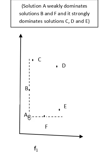
Figure 2 illustrates a particular case of the Pareto front in the presence of two objective functions

(Solution A weakly dominates solutions B and F and it strongly

dominatessolutions C, D andE)

f1 (minimize)





Fig. 2. The Pareto front in a two

objective space





































_

_













_























Pareto front

Dominated solutions

Pareto Optimal Solutions









f2

(

m

in

im

iz

e)

minimize f2

minimize

A B

F C

D

E

f

1

(minimiz

e)

f

2

(

m

ini

m

iz

e

)

[image:5.612.339.565.485.686.2]

(6)

International Journal of Emerging Technology and Advanced Engineering

222 We thus wish to determine the Pareto optimal set form the set P of all the feasible decision variable vectors that satisfy (6) to (8). It is to be noted that in practice, the complete Pareto Optimal set is not normally desirable (e.g. it may not be desirable to have different solutions that map to the same values in objective function space) or achievable. Thus a preferred set of Pareto optimal solutions should be obtained from practical point of view.

Particle Swarm Optimization (PSO)

James Kennedy and Russell C. Eberhart [1] originally proposed the PSO algorithm for single objective optimization. PSO is a population-based search algorithm based on the simulation of the social behavior of birds within a flock. Although originally adopted for neural network training and non-linear function optimization [18, 19], PSO soon became a very popular global optimizer, mainly in problems in which the decision variables are real numbers [19, 20]. It is worth noting that there have been proposals to use alternative encodings with PSO (e.g. binary [21] and integer [22]), According to Angeline [23] and as summarized by M. R. Sierra et al. [24], we can make two main distinctions between a PSO algorithm and an evolutionary algorithm (EA):

1.Evolutionary algorithms rely on three mechanisms in their processing: parent representation, selection of individuals, and the fine tuning of their parameters. In contrast, PSO relies on only two mechanisms, since it does not adopt an explicit selection function. The absence of a selection mechanism in PSO is compensated by the use of leaders to guide the search. However, there is no notion of offspring generation in PSO as with evolutionary algorithms.

2.Evolutionary algorithms use a mutation operator that can set an individual in any direction (although the relative probabilities for each direction may be different). PSO uses anoperator that sets the velocity of a particle toa particulardirection. This can be seen as a directional mutation operator in which the direction is defined by both the particle‟s personal best pbest and the global best (of the swarm) gbest. If the direction of pbest is similar to the direction of the gbest, the angle of potential directions will be small, whereas a larger angle will provide a larger range of exploration. In fact, the limitation exhibited by the directional mutation of PSO has led to the use of mutation operators similar to those adopted in evolutionary algorithms.

PSO has become so popular because its main algorithm is relatively simple and its implementation is, therefore, straightforward and it has been found to be very effective in a wide variety of applications with very good results at a very low computational cost [19, 25].

As a basic principle, in PSO, a set of randomly generated particles in the initial swarm are flown (have their parameters adjusted) through the hyper-dimensional search space (problem space) according to their previous flying experience. Changes to the position of the particles within the search space are based on the social-psychological tendency of individuals to emulate the success of other individuals. Each particle represents a potential solution to the problem being solved. The position of a particle is determined by the solution it currently represents. The position of each particle is changed according to its own experience and that of its neighbors. These particles propagate towards the optimal solution over a number of generations (moves) based on large amount of information about the problem space that is assimilated and shared by all members of the swarm. PSO algorithm finds the global best solution by simply adjusting the trajectory of each individual toward its own best location (pbest) and towards the best particle of the entire swarm (gbest) at each time step (generation). In this algorithm, the trajectory of each individual in the search space is adjusted by dynamically altering the velocity of each particle according to its own flying experience and the flying experience of the other particles in the search space.

The position vector and the velocity vector of the ith particle in the d-dimensional search space can be expressed

as

x

_i



(

x

_i₁

,

x

_i₂

,

x

_i₃

,...

x

_id

)

and

)

,...

,

(

_i₁ _i₂ _i₃ _id

i

v



respectively. According to a

user defined fitness function, the best position of each particle (which corresponds to the best fitness value

obtained by that particle at time t) is

)

,...,

,

(

i1 i2 i3 id

i

p



[It is also popularly

known as pbest] and the fittest particle found so far in the

entire swarm at time t is

)

,...,

,

(

_g₁ _g₂ _g₃ _gd

g

p



[It is also popularly known as gbest]. Then the new velocities and the new positions of the particles for the next fitness evaluation are calculated at time t+1 using the following two self-updating equations:

)) ( ) ( ()( 2 ))

( ) ( ()( 1 ) ( ) 1

(t wv t c1rand p t x t c2rand p t x t

vid   id  id  id  gd  id

(7)

International Journal of Emerging Technology and Advanced Engineering

223

x

_id

(

t



1 )



x

_id

(

t

)



v

_id

(

t

)

(10)

Where rand1 (.) & rand2(.) are two separately generated uniformly distributed random values in the range [0,1], w is inertia weight (or inertia factor) which is employed to control the impact of the previous history of velocities on the current velocity of a given particle, c1 & c2 are constants known as acceleration coefficients (or

learning

factors); c1 is the cognitive learning factor (or self confidence factor) which represents the attraction that a particle has toward its own success and c2 is the social learning factor (or swarm

confidence factor) which represents the attraction that a particle has toward the success of its neighbors. Normally, according to Hassan et al.[26], c1 ranges from 1.5 to 2, c2 ranges from 2 to 2.5 and w ranges from 0.4 to 1.4. From (9), it is observed that it has three components which are incorporated via a summation approach and effect the new search direction. The first component is known as current motion influence component which depends on previous velocity and provides the necessary momentum for particles to roam across the search space. The second

component is known as cognitive (or particle own memory

influence) component which represents the personal thinking of each particle and encourages the particles to move toward their own best positions found so far. The third component is known as social (or swarm influence) component which represents the collaborative effect of the particles, in finding the global optimal solution. This component always pulls the particles toward the global best particle found so far. PSO algorithms are quite promising in the applications to single objective optimization problems as compared to evolutionary algorithm (EA) techniques [19, 26, and 27]. These are very popular due to their simplicity in their implementations (a few parameters are needed to be tuned). A PSO algorithm is computationally cheap in the updating of the individuals per iteration, as the core updating mechanism in the algorithm relies only on two simple self-updating equations (9) and (10) as compared to using mutation and crossover operations in typical EA which requires a substantial computational cost.

PSO uses an operator that sets the velocity of a particle to a particular direction. This can be seen as a directional mutation operator in which the direction is defined by both the particle‟s personal best and the global best (of the swarm). If the direction of the personal best is similar to the direction of the global best, the angle of potential directions will be small, whereas a larger angle will provide a larger range of exploration.

In contrast, evolutionary algorithms use a mutation operator that can set an individual in any direction (although the relative probabilities for each direction may be different). In fact, the limitation exhibited by the directional mutation of PSO has led to the use of mutation operators (sometimes called turbulence operators) similar to those adopted in evolutionary algorithms.

The pseudo code for a basic PSO algorithm is illustrated in Algorithm 1.

Algorithm 1 General Single-Objective Particle Swarm Optimization Algorithm

01. Begin

02. Parameter settings and initialization of swarm 03. Evaluate fitness and locate the leader (i.e.

initialize pbest and gbest) 04. I = 0 /* I = Iteration count */

05. While (the stopping criterion is not met, say, I < Imax)

06. Do

07. For each particle

08. Update position & velocity (flight) as per equations (9) & (10)

09. Evaluate fitness

10. Update pbest

11. End For

12. Update leader (i.e. gbest) 13. I++

14. End While

15. End

First, the swarm is initialized. This initialization includes both positions and velocities. The corresponding pbest of each particle is initialized and the leader is located (the gbest solution is selected as the leader). Then, for a maximum number of iterations, each particle flies through the search space updating its position (using (9) and (10)) and its pbest and, finally, the leader is updated too.

Multi-Objective Particle Swarm Optimization (MOPSO)

(8)

International Journal of Emerging Technology and Advanced Engineering

224 However, since PSO and EA algorithms have structural similarities (such as presence of population searching for optima and information sharing between population members) and since EAs have already been successfully applied to multi-objective optimization problems, a transfer of PSO to the multi-objective domain can be a natural progression with some intelligent modifications in the basic PSO algorithm. Changing a PSO to a MOPSO requires a redefinition of what a guide is, in order to obtain a front of optimal solutions (Pareto front). In MOPSO, the Pareto-optimal solutions are used to determine the guide for each particle. A number of different studies have been published on Pareto approach based multi-objective PSO (MOPSO) [2, 27-48]

Each of these studies implements MOPSO in a different fashion. However, the PSO heuristic puts a number of constraints on MOPSO. In PSO itself the swarm population is fixed in size, and its members cannot be replaced, only adjusted by their pbest and gbest, which are by themselves easy to define. However, in order to facilitate an multi-objective approach to PSO, a set of non-dominated solutions (the best individuals found so far using the search process) must replace the single global best individual in the standard single-objective PSO case. Besides, there may be no single previous best individual for each member of the swarm. Choosing which gbest and pbest to direct a swarm member‟s flight is therefore important in MOPSO. Main focus of various MOPSO algorithms is how to select gbest and pbest with a separate divergence on whether an elite archive is maintained.

In order to apply the PSO strategy for solving multi-objective optimization problems, the original scheme has to be modified. The algorithm needs to search a set of different solutions (the so-called Pareto front) instead of a single solution (as in single objective optimization). We

need to apply Multi-Objective Particle Swarm

Optimization (MOPSO) to search towards the true Pareto front (non-dominated solutions). Unlike the single objective particle swarm optimization, the algorithm must have a solution pool to store non-dominated solutions found by searching up to stopping criterion (say, up to iteration Imax). Any of the solutions in the pool can be used as the global best (gbest) particle to guide other particles in the swarm during the iterated process. The plot of the objective functions whose non-dominated solutions are in the solution pool would make up for the Pareto front. The pseudo code for a general MOPSO is illustrated in Algorithm 2.

Algorithm 2 General Multi-Objective Particle Swarm Optimization Algorithm

01. Begin

02. Parameter Settings and initialize Swarm

03. Evaluate Fitness and initialize leaders in a leader pool or external archive

04. Archive the top best leader from the external

archive through evaluation of some sort of

quality measure for all leaders. 05. I = 0 /* I = Iteration count */

06. While (the stopping criterion is not met, say, I < Imax)

07. Do

08. For each particle

09. Select leader in the external archive

10. Update velocity

11. Update position

12. Mutate periodically /* optional */ 13. Evaluate Fitness

14. Update pbest

15. End for

16. Crowding of the leaders

17. Update the top best into external archive 18. I++

19. End While

20. Report results in the external archive

21. End

(9)

International Journal of Emerging Technology and Advanced Engineering

225 In the case of multi-objective optimization problems, each particle might have a set of different leaders from which just one can be selected in order to update its position. Such set of leaders is usually stored in a different place from the swarm that is called external archive. This is a repository in which the non-dominated solutions formed so far are stored. The solutions contained in the external archive are used as leaders when the positions of the particles of the swarm have to be updated. Furthermore, the contents of the external archive are also usually reported as the final output of the algorithm.

IV. ARTIFICIAL BEE COLONY OPTIMIZATION

Artificial Bee Colony (ABC) algorithm is one of the

most recently defined, swarm-based meta-heuristic

algorithm, introduced by Dervis Karaboga in 2005 [2], motivated by the intelligent behavior of honey bees for optimizing numerical problems. The algorithm is specifically based on the model proposed by Tereshko and Loengarov (2005) for the foraging behavior of honey bee colonies [1]. The main objective of this model is to find out how the synergistic information exchanging interactions between the individuals leads to globally intelligent selection of food sources in an unpredictable environment. To achieve this objective the model is developed which will be able to quickly select the “best” food sources in a changing environment of food sources, for this also Honeybees are considered because they are special among social insects for the importance of the nest as a center of

information and recruitment, since the foragers

communicate information about the environment to the nest.

The model proposed by Valery Tereshko & Andreas Loengarov (2005) [1] studied and found out that the model grouped bee activity into four compartments:

a. Unloading nectar from a source. b.Dancing for a source.

c. Feeding at a source. d.Following a dancer.

And corresponding probability functions need to consider for changing between these activities.

The minimal model of forage selection that leads to the emergence of collective intelligence consists of three essential components:

a. Food sources,

b.Employed foragers,

c. Unemployed foragers.

And defines two leading modes of the behavior:

a. Recruitment to a nectar source, b.Abandoned of a source.

a. Food Sources: The value of a food source to an insect depends on many factors including its proximity to the nest, richness or concentration of energy and the ease of extracting this energy.

To describe the “profitability” of a food source, the experimental research gives an idea that a richer source that is farther from the nest elicits the same profitability rating (as measured by number of waggle dances) as a source that is closer but not as rich, when they have the same net energetic efficiency. That is, when the energy gain minus the energy cost divided by the energy cost is the same – this value is used to describe food sources.

The model observes how insects react to food sources with different values of this quantity, and if they are always be able to select the “best” food sources in a changing environment.

b. Employed Foragers: Employed foragers are associated with a particular food source which they are currently exploiting or are “employed” at. They carry with them information about this particular source, its distance and direction from the nest and the profitability of the source. Employed foragers will share this information with a certain probability. The greater the profitability of the food source, the higher the probability the honeybee will do a waggle dance and share her information with her nest mates. Employed foragers are only locally informed – they know only of the food source they are currently exploiting and continue frequenting this food source until it is depleted, at which point they become unemployed foragers.

c. Unemployed Foragers: Unemployed foragers are looking for a food source to exploit. There are two types of unemployed foragers,

i) Scouts, who search the environment surrounding the nest (up to 14 km radius) in search of new food sources

ii)Onlookers, who wait in the nest and find a food source through the information shared by employed foragers

The model expresses the role of the nest as a reservoir of information, and the importance of information circulating freely throughout this reservoir.

(10)

International Journal of Emerging Technology and Advanced Engineering

226 So, the value of the source is expressed in the proportion of information about the source. Insects are recruited when information of a source reaches them; therefore, they are recruited to each source in proportion to the amount of the information circulating about that source.

How are bees recruited to more profitable sources? There is a greater probability of onlooker choosing more profitable sources because at any given time, more information is circulating about the more profitable sources. Employed foragers share their information with a probability which is proportional to the profitability of the food source, and the sharing of this information through the waggle dancing is longer in duration. So, at any given moment, the amount of information circulating about the food source will be proportional to the profitability of that source. Therefore, the recruitment is proportional to the profitability of a food source.

The behavior of the foragers can be explained properly below by taking an example.

Assume that there are two discovered food sources: A and B. At the very beginning, a potential forager will start as unemployed forager. That bee will have no knowledge about the food sources around the nest. There are two possible options for such a bee:

i) It can be a scout and starts searching around the nest spontaneously for a food due to some internal motivation or possible external clue.

ii)It can be a recruit after watching the waggle dances and starts searching for a food source.

After locating the food source, the bee utilizes its own capability to memorize the location and then immediately starts exploiting it. Hence, the bee will become an “employed forager”. The foraging bee takes a load of nectar from the source and returns to the hive and unloads the nectar to a food store.

After unloading the food, the bee has the following three options:

i) It becomes an uncommitted follower after abandoning

the food source (UF).

ii)It dances and then recruits nest mates before returning to the same food source (FE1).

iii) It continues to forager at the food source without recruiting other bees (EF2).

Here not all bees start foraging simultaneously. The experiments confirmed that new bees begin foraging at a rate proportional to the difference between the eventual total number of bees and the number of present foraging.

The self organization of the honey bees relies on the following properties:

i) Positive Feedback: As the nectar amount of food sources increases, the number of onlookers visiting them increases.

ii)Negative Feedback: The exploration process of a food source abandoned by bees is stopped.

iii) Fluctuations: The scouts carry out a random search process for discovering new food sources.

iv) Multiple Interactions: Bees share their information about food source positions with their nest mates on the dance area.

ABC Algorithm

A particular intelligent behavior of a honey bee swarm, foraging behavior, is considered in the Artificial Bee Colony Algorithm for solving multidimensional and multimodal optimization problems. In this model also the artificial bees consists of three group of bees: employed bees, onlookers and scouts.

Steps of the ABC algorithm

Send the scouts onto the initial food sources

REPEAT

Send the employed bees onto the food sources and determine their nectar amounts

Calculate the probability value of the sources with which they are preferred by the

Onlooker bees

Stop the exploitation process of the sources abandoned by the bees

Send the scouts into the search area for discovering new food sources, randomly

Memorize the best food source found so far

UNTIL (requirements are met)

Each cycle of the search consists of three steps:

i) Moving the employed bees onto the food sources and

calculating their nectar amounts

ii)Selecting of the food sources by the onlookers after sharing the information of employed bees and calculating their nectar amounts

iii) Determining the scout bees and directing them onto possible food sources.

(11)

International Journal of Emerging Technology and Advanced Engineering

227 Stage 2: At the second stage, after sharing the information, every employed bee goes to the food source area visited by her at the previous cycle since that food source exists in her memory and then chooses a new food source by means of visual information in the neighborhood of the present one.

Stage 3: At the third stage, an onlooker prefers a food source area depending on the nectar information distributed by the employed bees on the dance area. As the nectar amount of a food source increases, the probability with which that food source is chosen by an onlooker increases. Hence, the dance of employed bees carrying higher nectar recruits the onlookers for the food source areas with higher nectar amount. After arriving the selected area, she chooses a new food source in the neighborhood of the one in the memory depending on visual information. Visual information is based on the comparison of food source positions. When the nectar of a food source is abandoned by the bees, a new food source is randomly determined by a scout bee and replaced with the abandoned one. In the model, at each cycle at most one scout goes outside for searching a new food source and the number of employed and onlooker bees were equal. The flow chart of the ABC algorithm can be presented

in the

figure 3.

Key Parameters, Constraints and Measures of ABC algorithm:

For the implementation of ABC algorithm there are several parameters and constraints to be followed, they are summarized as below

a)A food source position represents a possible solution to the problem to be optimized.

b)The amount of nectar of a food source corresponds to the quality (fitness) of the solution represented by that food source.

c)

The number of employed bees or the onlooker bees is

equal to the number of solutions in the population

.

d)Onlookers are placed on the food sources by using a

probability based selection process. As the nectar amount of a food source increases, the probability value with which the food source is preferred by onlookers increases.

e)Every bee colony has scouts that are the colony‟s explorers. The explorers do not have any guidance while looking for food. Since they are primarily concerned with finding any kind of food source, so the scouts are characterized by low search costs and a low average in food source quality.

In the case of artificial bees, the artificial scouts could have the fast discovery of the group of feasible solutions or a task. In this work, one of the employed bees is selected and classified as the scout bee. The selection is controlled by a control parameter called “limit”. If a solution representing a food source is not improved by a predetermined number of trials, then that food source is abandoned by its employed bee and the employed bee is converted to a scout.

f) The number of trials for releasing a food source is equal to the value of “limit” which is an important control parameter of ABC.

g)In the ABC algorithm, while onlookers and employed

bees carry out the exploitation process in the search space, the scouts control the exploration process. h)In the case of real honey bees, the recruitment rate

represents a “measure” of how quickly the bee swarm locates and exploits the newly discovered food source.

Artificial recruiting processes similarly represent the “measurement” of the speed with which the feasible solutions or the optimal solutions of the difficult optimization problems can be discovered.

i) The survival and progress of the real bee swarm depended upon the rapid discovery and efficient utilization of the best food sources.

j) There are four control parameters used in the ABC algorithm:

1.The number of food sources which is equal to the

number of employed or onlooker bees (SN), 2.The value of limit, and

(12)

International Journal of Emerging Technology and Advanced Engineering

228 Flow Chart of ABC algorithm

Application of ABC

a. Engineering design – where problems normally have mixed (continuous & discrete) design variables,

nonlinear objective functions and nonlinear

constrains. Since constrains are very important in engineering design problems, if it is very hard to satisfy, which makes the search difficult and inefficient. Different deterministic as well as stochastic algorithms have been developed for solving constrained optimization problems. But deterministic approaches such as sequential quadratic programming methods and generalized reduced gradient methods have some limitations which often require making several assumptions that are difficult to justify in many situations, therefore their applicability is limited. On the other hand, stochastic optimization algorithms such as genetic algorithms, simulated

annealing algorithms, evolution strategies,

evolutionary programming and particle swarm optimization have been successfully applied for solving constrained optimization problems [6].

b. Distribution Network Configuration – to solve the network reconfiguration problem in a radial distribution system which considers the objectives such as minimization of real power loss, voltage profile improvement and feeder load balancing subject to the radial network structure in which all loads must be energized [9].

c. Wireless Sensor Networks (WSNs) – the optimization techniques are used in the dynamic deployment of WSNs that improves the coverage of the network in a 2-dimensional space [11].

d. Dimensionality Reduction – to obtain more accurate reduct, Rough Set-based Attribute Reduction (RSAR) is used for feature selection [12].

Economic fields:

a. Economic Load Dispatch (ELD) – to solve the

economic dispatch problem with non-smooth cost function or valve-point effect for saving millions of dollars per year in production cost [17].

b. Market Segmentation – to solve problems of

segmenting market on the basis of effectivetargeting and predicting of potential customers in new and competitive commercial framework [18].

Medical fields:

a. MRI fuzzy segmentation of Brain Tissue – to solve the goal in segmentation process is to partition a

medical image into regions that are homogeneous

with respect to characteristics [19].

Start

Send the scouts into the initial food source

Send employed bees onto food source

Determine nectar amount

Portability value higher?

On looker bees preferred the food source

yes

Send scouts for searching new food source

Memorize the Food Source

(13)

International Journal of Emerging Technology and Advanced Engineering

229 V. CONCLUSION

PSO is a computational intelligence based techniques that is not largely affected by the size and nonlinearity of the problem, and can converge to the optimal solution in many problems were most analytical methods fail to converge [11]. It is a stochastic optimization technique [12] inspired by social behavior of bird flocking or fish schooling [13]. It is initialized with a group of random particles (solutions) and then searches for optima by updating generations. Moreover, PSO has some advantages over other similar optimization techniques such as: i) It is easier to implement and there are fewer parameters to adjust. ii) In PSO, every particle remembers its own previous best value as well as the neighborhood best. iii) PSO is more efficient in maintaining the diversity of the swarm since all the particles use the information related to the most successful particle in order to improve themselves [14] [15].

Another popular but recent algorithm which is being in use is ABC algorithm, which was proposed in [16]. ABC is modeled on two processes: sending of bees to nectar (food source) and desertion of a food source. While in other swarm intelligence algorithms, the swarm represents the solution, in ABC the food source gives the solution while bees act as variation agents responsible for generating new sources of food [17] [18]. Three types of bees, namely, employed, onlooker and scout bees, aid in reaching the optimal solution. This algorithm is very simple when compared to existing swarm algorithms. These algorithms have recently been shown to produce good results in a wide variety of real-world applications.

REFERENCES

[1 ] J. Kennedy and R. C. Eberhart, ”Particle Swarm Optimization”, Proceedings of the IEEE International Conference on Neural Networks, Perth, Australia, pp. 1942-1948, 1995.

[2 ] J.Moore, R. Chapman and G. Dozier, “Multi-Objective Particle Swarm optimization”, ACM, pp. 56-57, 2000.

[3 ] K. Deb. Optimization for Engineering Design: Algorithms and Examples. Prentice-Hall, New Delhi, 1995.

[4 ] S. S. Rao. Optimization: Theory and Applications. Wiley, Nework, 1984.

[5 ] G. V. Reklaitis, A. Ravindran and K. M. Ragsdell. Engineering Optimization Methods and Applications. Wiley, New York, 1983. [6 ] V. Chankong and Y.Y. Haimes. Multi-objective Decision Making

Theory and Methodology. North-Holland, New York, 1983. [7 ] M. Ehrgott. Multi-criteria Optimization. Springer, Berlin, 2000. [8 ] K. Miettinen. Nonlinear Multi-objective Optimization. Kluwer,

Boston, 1999.

[9 ] Y. Y. Haimes, L.S. Lasdon and D.A. Wismer,“On a Bicriterion Formulation of the Problems of Integrated System Identification and System Optimization”, IEEE Transactions on Systems, Man, and Cybermetics, Vol. 1, Sec. 3, pp. 296-297, 1971.

[10 ]R.L. Kenney and H. Raiffa. Decisions with Multiple Objectives: Preferences and Value Tradeoffs. Wiley, New York, 1976. [11 ]A. Charnes, W. Coope, and R. Ferguson, “Optimal Estimation of

Executive Compensation by Linear Programming”, Management Sciences, Vol. 1, Sec. 2, pp. 138-151, 1955.

[12 ]J.P. Ignizio. Goal Programming and Extensions. Lexington, MA: Lexington Books, 1976.

[13 ]J.P. Ignizio, “A Review of Goal Programming: A Tool for Multi-objective Analysis”, Journal of Operations Research Society, Vol. 29, Sc. 11, pp. 1109-1119, 1978.

[14 ]S. M. Lee. Goal Programming for Decision Analysis. Auerbach Publishers, Philadelphia, 1972.

[15 ]C. Romero. Handbook of Critical Issues in Goal Programming. Pergamon Press, Oxford, UK, 1991.

[16 ]V. Tereshko, A. Loengarov, “Collective Decision-Making in Honey Bee Foraging Dynamics”, Computing and Information Systems Journal, ISSN 1352-9404, vol. 9, No. 3, October 2005.

[17 ]Dervis Karaboga, “An Idea Based On Honey Bee Swarm For Numerical Optimization”, Technical Report-TR06, October 2005. [18 ]Dervis Karaboga, Bahriye Basturk, “A powerful an efficient

algorithm for numerical function optimization: artificial bee colony (ABC) algorithm”, Springer Science + Business Media B.V. 2007, published online: 13 April 2007.

[19 ]Dervis Karaboga, Bahriye Akay, “A survey: algorithms simulating bee swarm intelligence”, Springer Science + Business Media B.V. 2007, published online: 28 October 2009.

[20 ]Karaboga D, Basturk B (2007a), “Artificial bee colony (ABC) optimization algorithm for solving constrained optimization problems. In: Advances in soft computing: foundations of fuzzy logic and soft computing, LNCS, vol 4529/2007. Springer-Verlag, pp 789-798.

[21 ]Ivona Brajevic, Milan Tuba, and Milos Subotic, “Performance of the improved artificial bee colony algorithm on standard engineering constrained problems”, International Journal of Mathematics and Computers in Simulation, issue 2, volume 5, 2011.

[22 ]D. Karaboga and B. Basturk, “On the performance of artificial bee colony (ABC) algorithm”, Applied Soft Computing 8(2008), pp. 687-697, 2008.

[23 ]D. Karaboga, B. Basturk and B. Akay, “Artificial Bee Colony Algorithm on Training Artificial Neural Networks, Signal Processing and Communications Applications”, SIU 2007, IEEE 15th. 11-13 June 2007, Page(s): 1-4, doi:10.1109/SIU.2007.4298679.

[24 ]R. Srinivasa Rao, S.V.L. Narasimham, M. Ramalingaraju, “Optimization of Distribution Network Configuration for Loss Reduction Using Artificial Bee Colony Algorithm”, World Academy of Science, Engineering and Technology, 2008.

[25 ]Mustafa M. Noaman, Ameera S. Jaradat, “Solving Shortest Common Supersequence Problem Using Artificial Bee Colony Algorithm”, The Research Bulletin of Jordan ACM, ISSN: 2078-7952, Volume II (III), 2011.

[26 ]Celal Ozturk, Dervis Karaboga, Beyza Gorkemli, “Artificial bee colony algorithm for dynamic deployment of wireless sensor networks”, Turk J Elec Eng & Comp Sci, Vol.20, No.2, 2012. [27 ]Nambiraj Suguna and Keppana Gowder Thanushkodi, “An

(14)

International Journal of Emerging Technology and Advanced Engineering

230

[28 ]Chunfan Xu, Haibin Duan, “Artificial bee colony (ABC) optimized edge potential function (EPF) approach to target recognition for low-altitude aircraft”, Pattern Recognition Lett. (2010).

[29 ]Anguluri Rajasekhar, Millie Pant, Ajith Abraham, “Cauchy Movements for Artificial Bees for Finding Better Food Sources”, Third World Congress on Nature and Biologically Inspired Computing, 2011.

[30 ]Wenping Zou, Yunlong Zhu, Hanning Chen and Tao Ku , “Clustering Approach Based On Von Neumann Topology Artificial Bee Colony Algorithm”.

[31 ]Wenping Zou, Yunlong Zhu, Hanning Chen and Xin Sui, “A Clustering Approach Using Cooperative Artificial Bee Colony Algorithm”, Hindawi Publishing Corporation, Discrete Dynamics in Nature and Society, Volume 2010, Article ID 459796, 16 pages, doi:10.1155/2010/459796.

[32 ]S. Hemamalini and Sishaj P Simon, “Economic Load Dispatch with Valve-Point Effect using Artificial Bee Colony Algorithm”, XXXII National systems Conference, NSC 2008, December 17-19, 2008. [33 ]Babak Amiri and Mohammad Fathian, “Integration of Self