A COMBINED FORECASTING METHOD OF WIND POWER
CAPACITY WITH DIFFERENTIAL EVOLUTION
ALGORITHM
1JIANJUN WANG, 1HONGYANG ZHANG, 1ZHANGYI PAN, 2LI LI
1
School of Economic and Management Administration, North China Electric Power University, Beijing 102206, China
2School of Economics & Business Administration, Beijing Information Science & Technology University,
Beijing 100085, China
ABSTRACT
As wind power is a mature and important renewable energy, wind power capacity forecasting plays an important role in renewable energy generation’s plan, investment and operation. Combined model is an effective load forecasting method; however, how to determine the weights is a hot issue. This paper proposed a combined model with differential evolution optimizing weights. The proposed model can improve the performance of each single forecasting model of regression, BPNN and SVM. In order to prove the effectiveness of the proposed model, an application of the China’s wind power capacity was evaluated from 2000 to 2010. The experiment results show that the proposed model gets the maximum mean absolute percentage error (MAPE) value 1.791%, which is better than the results of regression, BPNN and SVM.
Keywords: Capacity Forecasting, Differential Evolution Algorithm, Wind Power
1. INTRODUCTION
Renewable energy generation is an important way for electricity power industry to achieve the energy saving goal, which helps China finish the promise of decreasing the carbon emissions per unit of GDP by 40-45% in 2020 compared with 2005. As wind power generation is the most mature renewable energy technology in the renewable energy generation, it has been developed rapidly. From 2000 to 2008, the increasing rate of wind power generation in main developed country has been improved more than 20%.
Wind power forecasting problem is one of the load forecasting problems, which is a traditional issue but a difficult problem, because it always influenced by many factors. Many of countries in the world have focused on the load forecasting in the last decades such as the regressive method [1], autoregressive moving average model (ARMA)[2] and intelligent load forecasting algorithms.
The artificial neural networks (ANNs) became one of the most popular intelligence methods in last decade because it can consider the non-linear factors and only a three-layer neural network can achieve any accuracy degree of any continuous function mapping by the Kromogol's theorem. M.
Beccali proposed a group of neural networks for a suburban area's electric demand forecasting and obtained a good forecasting accuracy [3]. In this field, Henrique Steinherz Hippert gave a very excellent review on the neural networks for load forecasting [4], and in the review, he pointed out that the back propagation artificial neural network (BPNN) is the most popular algorithm in the ANNs.
Furthermore, with support vector regression (SVR) method proposed by Vapnik in 1998, SVR become the other popular method for load forecasting. Support vector regression (SVR) uses the structural risk minimization principle to minimize the generalization errors principle and overcome the local optimal solution problem. B.J. Chen won a load forecasting competition organized by EUNITE network in 2001 by a SVR model [5]. P.F. Pai and W.C. Hong combined several intelligence algorithms such as genetic algorithm (GA), simulated annealing (SA) and immune algorithm with the SVR model to forecast Taiwan's annual electric load, and they obtained a very good performance in case study, it also shows that SVR models outperform ARIMA and ANN models [6].
ARIMA[7] model, ANN model[8,9], GMDH model[10] and so on. It regrets that few researches pay attention to the forecasting problem about wind power capacity, which plays an important role for the wind power construction plan, investment and operation. And these papers are all focused on using a single model to solve the wind power forecasting, some forecasting scholars have been pointed out that a single model’s performance is worse than combined models’. The reasons are as follows: first, the combined model can reduce disadvantage of any a single model; second, the errors of combined model are always smaller than each single model’s. Therefore, this paper proposed a combined forecasting model of wind power capacity with differential evolution algorithm to solve the problem.
This paper is organized as follows. In section 2, the combined forecasting model with differential evolution algorithm is given. In section 3, the experimental results of comparing the algorithm proposed in this paper with other algorithms are presented. Finally, our work of this paper is summarized in the last section.
2. A COMBINED FORECASTING MODEL
WITH DIFFERENTIAL EVOLUTION ALGORITHM
In practice, a load forecasting problem can use different load forecasting models, so the load forecasting accuracy are also different. How to choose the best forecasting model is a difficult problem.
Using combined forecasting model can solve the above problem. A combined forecasting model consists of two or more forecasting models and each model has a certain weights, a combined forecasting model can be described as follows:
Suppose that fi is forecasting results of the ith
method, y is the actual data. The combined forecasting model yˆ can be expressed by
1 ˆ
n i i i
y w f
=
=
∑
(1)In which, wi is the weight of the ith method, and
an optimization problem of the combined model need satisfy the following model.
1
: ( )
n i i i
Min MSE y w f
=
−
∑
(2)1
. . 1; 0
n
i i
i
s t w w
=
= ≥
∑
The key problem of the combined model is to determine the weight. The weight determine methods can be divided into two categories, one is fixed weight method, which determined the weight as a fixed number, and the other is transformable weight method, which determined the weight as a function of the time. The fixed weight determined model is the most popular method because it is simple and easy to apply, and it is suitable for using intelligence algorithm such as genetic algorithm, particle swarm optimization to solve the problem.
Differential evolution (DE) algorithm is one of the evolutionary algorithms, which was proposed by Storn and Price in order to solve the Chebychev Polynomial fitting problem at first, it becomes one of the most popular optimization algorithms. As other evolution algorithms such as genetic algorithm (GA), DE is also population based algorithm, which contains mutation, crossover and selection steps. However, compare with other evolution algorithms, DE is easy to implement, it needs fewer parameters and exhibits fast convergence. The detail working steps are as follows [11]:
Step 1.Parameters initialization
The main parameters of DE algorithm are population size N, length of the chromosome D, the mutation factor F, the crossover rate C and the maximum generations number g. the mutation factor F is selected in [0, 2], the crossover rate C is selected in [0, 1] and the larger C is always easy to premature and convergence faster.
Step 2.Population initialization
Set g=0. Generate a N*D matrix with uniform probability distribution random values. The generation method is
( [ ] [ ]) [ ]
ij
X =rand⋅ high j −low j +low j (3)
In which, i=1, 2,,N , j=1, 2,,D,rand is a random number with a uniform probability distribution, and high[j], low[j] is the upper bound and lower bound of the jth column, respectively.
Step 3.Population evolution
Calculate and record fitness values of all the individuals.
Step 4.Mutation operation
This operation uses two random chosen vectors
Xb,Xc to produce a mutant X’a' vector as follows:
' ( )
a a b c
In which, F is the mutation factor in the range [0,1], a b c, , ∈{1, 2,, }N are randomly chosen and they must keep different from each other.
Step 5.Crossover operation
Crossover operation can increase the diversity of the population, and the equation is shown as follows.
' '
'
( ) ( ) ( ) ( )
( ) ( )
b a
b a
X j X j if rand j C or j randn j
X j X j otherwise
= ≤ =
=
(6)
Where j is the gene location of a population,
rand(j) is a random number and rand(j) is also a
random integer in the range of [1,D], ensures that at least one element of the population can get the crossover operation. C is the crossover rate in [0,1].
Step 6.Selection operation
Selection operation retains the better offspring in the next generation. The selection principle is the fitness values, if the offspring’s fitness value f(Ui,G)
is better than the parent’s f(Xi,G) , the offspring Ui,G
would select, otherwise, the parent Xi,G would
retain.
, , ,
, 1 ,
( ) ( )
i G i G i G
i G
i G
U if f U f X
X
X otherelse
+
<
=
(2)
DE algorithm has the better performance than GA and PSO algorithms in the examination of the 34 widely used benchmark functions [12]. According to the study, DE algorithm is stable and it can obtain a better solution than other algorithms, and the experiment results are also shown that DE can get the nearest optimal solution then PSO and GA algorithm. Therefore, the DE algorithm will be used to solve the weight determining problem, whose fitness function is employed the mean absolute percentage error function (MAPE), which is common used in load forecasting performance evaluation.
1
1 ( ) ( ) 100% ( )
n
i
A i F i
MAPE
n = A i
−
=
∑
× (2)Where A(i) is the actual value, F(i) is the forecasting value and n is the total numbers.
3. A NUMERIC EXAMPLE
In this case, we use the annual wind power capacity of China from 2000 to 2010, which is shown in Figure 1.
20000 2001 2002 2003 2004 2005 2006 2007 2008 2009 2010 0.5
1 1.5 2 2.5 3 3.5 4 4.5x 10
4
Year
Load(
M
W
)
Figure 1: The wind power capacity of China from 2000 to 2010
It is clearly seen that the curve appears an exponential curve character, so we are using the
ln(x) value as the dependent variable in the single
forecasting models. And the single forecasting models are chosen as regression model, back propagation neural network (BPNN) and support vector machine(SVM) models, because these models are all the popular single models in load forecasting.
In BPNN forecasting model, the node number of input layer is xt-3, xt-2, xt-1, the hidden layer number
is five and the output node is xt . In SVM
forecasting model, the input variables are also xt-3,
xt-2, xt-1, and the output node is also xt, the same as
BPNN model, but the parameters is 0.1,C 1000, 0.5
δ = = µ= , because these three
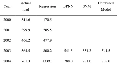
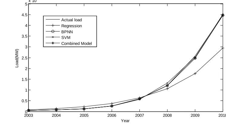
[image:3.612.313.513.72.283.2]parameters are best performances in the experiments. The proposed combined weight of regression, BPNN and SVM, which determined by DE algorithm with default parameters, are 0, 0.9931 and 0.0069 respectively. The final results are all shown in Table 1 and Figure 2.
Table 1. The Actual Load And Forecasting Results Of Regression, ANN, SVM And Combined Model
Year Actual
load Regression BPNN SVM
Combined Model
2000 341.6 170.5
2001 399.9 285.5
2002 466.2 477.9
2003 564.5 800.2 541.5 551.2 541.5
[image:3.612.310.513.606.722.2]2005 1268.2 2243.0 1239.8 1247.4 1239.9
2006 2555.8 3755.4 2558.5 2494.8 2558.1
2007 5867 6287.4 5868.2 5699.5 5867.0
2008 12020.7 10526.8 12021.2 13162.2 12029.1
2009 25823.9 17624.5 24825.0 25204.8 24827.6
2010 44751.89 29507.8 44637.1 45047.9 44639.9
MAPE -- 33.387% 1.793% 2.972% 1.791%
From the determined weight of DE algorithm, it can be clearly seen that BPNN model gets the maximum weight, SVM follows, and the regression model’s weight is zero. The better the performance is, the greater the weight is. It proves that DE algorithm is effective.
4. CONCLUSION
The proposed combined model integrates the regression, BPNN and SVM models. With using DE algorithm to determine the weight, it can
improve the load forecasting performance. In the experiment, the proposed method gets the minimum MAPE values, which verifies the proposed method’s effectiveness in wind power capacity forecasting.
ACKNOWLEDGEMENTS
This work was supported by NSFC under Grant No. 71071052, 70671039 and the Fundamental research funds for the central universities (12QN27).
.
20030 2004 2005 2006 2007 2008 2009 2010 0.5
1 1.5 2 2.5 3 3.5 4 4.5
5x 10
4
Year
Load(
M
W
)
Actual load Regression BPNN SVM
[image:4.612.107.480.380.590.2]Combined Model
REFERENCES:
[1] A. Goia, C. May, G. Fusai, “Functional clustering and linear regression for peak load forecasting”, International Journal of
Forecasting, Vol.26, No. 4, 2010, pp. 700-711.
[2] S.Sp. Pappas, L. Ekonomou, D.Ch. Karamousantas, G.E. Chatzarakis, S.K. Katsikas, P. Liatsis, “Electricity demand loads modeling using AutoRegressive Moving Average (ARMA) models”, Energy, Vol. 33, No 9, 2008, pp.1353-1360.
[3] M. Beccali, M. Cellura, V. Lo Brano, A. Marvuglia, “Forecasting daily urban electric load profiles using artificial neural networks”,
Energy Conversion and Management, Vol.
45 ,No. 18-19, 2004,pp. 2879-2900.
[4] H. S. Hippert, C. E. Pedreira, R. C. Souza, “Neural networks for short-term load forecasting: a review and evaluation”, IEEE
Transactions on Power Systems,Vol.16, No. 1,
2001, pp. 44-55.
[5] B.-J. Chen, M.-W. Chang, C.-J. Lin, “Load forecasting using support vector machines: A study on EUNITE Competition 2001”, IEEE
Transactions on Power Systems, Vol.19, No.4,
2004, pp. 1821-1830
[6] W.-C. Hong, “Electric load forecasting by support vector model”, Applied Mathematical
Modelling,Vol.33, No.5, 2009 , pp. 2444-2454.
[7] E. Erdem, J. Shi, “ARMA based approaches for forecasting the tuple of wind speed and direction”, Applied Energy, Vol.88, No. 4, 2011, pp. 1405-1414.
[8] M. Monfared, H. Rastegar, H. M. Kojabadi, “A new strategy for wind speed forecasting using artificial intelligent methods”, Renewable
Energy, Vol. 34, No. 3, 2009, pp. 845-848.
[9] Z. H. Guo, W. G. Zhao, H. V. Lu , J. Z. Wang, “Multi-step forecasting for wind speed using a modified EMD-based artificial neural network model”, Renewable Energy, Vol. 37, No. 1, 2012, pp. 241-249.
[10] R.E. Abdel-Aal, M.A. Elhadidy, S.M. Shaahid, “Modeling and forecasting the mean hourly wind speed time series using GMDH-based abductive networks”, Renewable Energy, Vol. 34, No. 7, 2009, pp. 1686-1699.
[11] J.J. Wang, L. Li, D.X. Niu, Z.F. Tan, “An annual load forecasting model based on support vector regression with differential evolution algorithm”, Applied Energy, Vol. 94, 2012, pp. 65-70.
[12] L. dos Santos Coelho, V. C. Mariani, “Combining of chaotic differential evolution and quadratic programming for economic dispatch optimization with valve-point effect”,
IEEE Transactions on Power Systems,Vol. 21,