http://www.sciencepublishinggroup.com/j/ajrs doi: 10.11648/j.ajrs.20180601.17
ISSN: 2328-5788 (Print); ISSN: 2328-580X (Online)
Land Use Detection Using Remote Sensing and GIS (A
Case Study of Rawalpindi Division)
Muhammad Zubair Iqbal
1, Muhammad Javed Iqbal
21
University Institute of Information Technology, Peer Mahar Ali Shah Arid Agriculture University, Rawalpindi, Pakistan
2Department of Geo- Informatics, Peer Mahar Ali Shah Arid Agriculture University, Rawalpindi, Pakistan
Email address:
To cite this article:
Muhammad Zubair Iqbal, Muhammad Javed Iqbal. Land Use Detection Using Remote Sensing and GIS (A Case Study of Rawalpindi Division). American Journal of Remote Sensing. Vol. 6, No. 1, 2018, pp. 39-51. doi: 10.11648/j.ajrs.20180601.17
Received: February 11, 2018; Accepted: March 8, 2018; Published: April 23, 2018
Abstract:
Change detection is a process of identifying variations in the substances or marvels which are supposed in the different time interims. This study takes the spatial-temporal dynamics of land use/cover change in Rawalpindi division Punjab Pakistan, using satellite imageries of two different years 2000, 2008. Supervised classification method was applied to demonstrate the object in a certain period of time. The method represents the vegetation index of differencing through object-based and supervised classification along with expert knowledge of GIS. This method gave different results in terms of land cover area, and it's generally concluded most accurate result from spatial images of medium resolution. The result of this process will be used for agriculture, urban and environmental changes in the various time periods. All information leads to the conclusion that surface under land class tabulation will be generated. The result shows vegetation, forest degradation and increase in built-up area with seasonal urbanization. Maps of the land use/land cover changes available in GIS platform can be used for the enhancement of the available tools for urban planning and environmental factor in the area.Keywords:
Imagery, Supervised Classification, Land Use Planning, Remote Sensing, Geographical Information System (GIS)1.
Introduction
Land use change detection is the process detaching difference between objects and phenomena which can be observed in different time breaks. Its aim is to select and put into practice those land uses, which will meet the need of the people by securing resources for the future (Singh R B, Dilip Kumar 2012). In Pakistan, land resources have reached a critical stage due to the increasing population especially in urban cities. A comprehensive approach toward conservation of land resources, which also counts the vulnerable environment. The changes on earth apparently, could be related to the natural dynamics of human happenings. Apart from the seasonal rainfall and possible interchangeable factors of rainfall, flood and drought that influence changes in natural vegetation, agriculture land and vice versa are necessary. Timely and accurate change detection of the earth surface condition provides better understandings of the interaction between human and natural phenomena for better
management (Tricart E 2007 and Boori M. S., Choudhary K., Kupriyanov A., Kovelskiy V. 2016). Over the last twenty years, especially in the upper and northern and central Punjab, has the worst rate of urbanization and has been subjected to both natural and human factors such as droughts, cities migration, large population and cover refers to the physical characteristics of the earth surface. This will be captured in the distribution of vegetation, area of forest, water, urbanization and other physical features of the land for settlements.
40 Muhammad Zubair Iqbal and Muhammad Javed Iqbal: Land Use Detection Using Remote Sensing and GIS (A Case Study of Rawalpindi Division)
C 2013 and Rogan J., Eastman J. R., Turner II B. L 2015). Remote sensing and Geographical Information system provides dynamic tools which can be applied in the analysis at the district as well as micro level. Remote sensing provides synoptic view and multi- historical land uses/ land cover data (R. K. Nigam 2000). Remote sensing and Geographical Information System based technologies may be applied to an area in order to generate a sustainable development plan (Singh R B and Dilip Kumar 2012). Land use planning, based on land resource evaluation and spatial direction of planning as part of GIS ensures appropriate land allocation in order to achieve sustainable agriculture (Andy Bhermana 2013).
The objective of the study is:
1- Visualize the change detection of the land use in agriculture and other different prospective.
2- To monitor the land cover changes using GIS and Remote Sensing.
3- Suggestions for improved management of the natural resources through classification.
4- An analysis of land use change detection for different years and its sum to control further urbanization into the agricultural land.
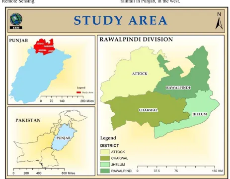
Rawalpindi is the region in Punjab Pakistan (Figure 1). It is the most populous region in Punjab province of Pakistan and lying between 32º - 30" N to 34º latitude and from 71º - 45" E to 73º - 45" E longitudes. It is situated at an elevation of 472.2 to 609.6 meter above sea level lying to the south of Pakistan's majestic northern mountain range (Kala Chitta Range and the Margalla Hills); the salt range is present on the southern side whereas in the west is the River Indus and in the east is the River Jhelum. The total area is 22,254 km (8,592 sq. mi). In general, it has a Mediterranean climate with hot, dry summer and mild rainy winter but the climate of Rawalpindi dry desert in the east to the area of highest rainfall in Punjab, in the west.
Figure 1. Map of Study Area.
2. Material and Method
The data used in this paper was divided into two categories; first satellite data and second ancillary data. Satellite data further subdivided into multi-spectral data acquired by the land set that’s freely provided by USGS glovis. Ancillary data include ground truth for the land use
1. Red - 0.61 to 0.68 µm
2. Near-infrared - 0.78 to 0.89 µm 3. Short-wave infrared - 1.58 to 1.75 µm
4. Blue band - 0.43 to 0.47 µm, for atmospheric corrections.
The red and near-infrared bands are used by VITO for making daily and S10 Normalized Difference Vegetation Index (NDVI) composites.
2.1. Satellite Images
This case study used the images of two separate cloud-free Landsat TM data from Landsat 4-5 Thematic Mapper (TM) and Landsat 7. The main difference between these sensors is in the numbers of the spectral ranges but also in the radiometric resolution, which is 8 bits for the Landsat 4-5, and 8-bits for the Landsat 7 ETM + (Table 1). The fact that different sensors with different spectral and radiometric resolution are used for change detection process.
Table 1. Characteristics of the Landsat datasets used in the study.
Landsat 4-5 ETM+ Bands (mm)
Band 1 30 m Blue 0.441 - 0.514 Multispectral
Band 2 30 m Green 0.519 - 0.601 Multispectral
Band 3 30 m Red 0.631 - 0.692 Multispectral
Band 4 30 m NIR 0.772 - 0.898 Multispectral
Band 5 30 m SWIR-1 1.547 - 1.749 Multispectral
Band 6 60 m TIR-1 10.31 - 12.36 Thermal high - low gain
Band 7 30 m SWIR-2 2.064 - 2.345 Multispectral
Landsat 7 ETM+ Bands (mm)
Band 1 30 m Coastal/Aeros 0.435 - 0.451 Multispectral
Band 2 30 m Blue 0.452 - 0.512 Multispectral
Band 3 30 m Green 0.533 - 0.590 Multispectral
Band 4 30 m Red 0.636 - 0.673 Multispectral
Band 5 30 m NIR 0.851 - 0.879 Multispectral
Band 6 30 m SWIR-1 1.566 - 1.651 Thermal high - low gain
Band 7 30 m SWIR-2 2.107 - 2.294 Multispectral
Band 8 15 m Pan 0.520 - 0.901 Panchromatic
The stepwise process of land covers changes mapping process here. The whole process is categorized into given steps as mentioned below.
2.2. Pre-Processing
Due to the inaccuracy of the sensing devices and smaller or bigger systematical mistakes, the preprocessing is an inevitable step in the change detection. As are the ETM+ images, Landsat 5 TM images are processed using standard geometric and radiometric correction methods and are corrected for possible geolocation errors due to terrain effect using the 1-arc second NED dataset, yielding TM DN images. With the TM sensor and the ETM+ sensor being geometrically and radiometrically compatible, the above Landsat 7 preprocessing procedures (including converting DN to at-satellite reflectance and tasseled cap transformation) are also applied to Landsat 5 TM images. To take advantage of the superior radiometric calibration of ETM+, however, TM DN (DN5) is first converted (U.S. Geological Survey).
ETM+ DN (DN7) using the following equation:
DN7 = DN5 (slope + intercept)
Where the slope and intercept values are as follows according to (Vogel Mann) at all. (2001):
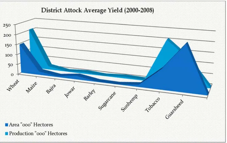
Table 2. Slope and Intercept Values of the Bands.
Band # Slope Intercept
1 0.9398 4.7289
2 1.7731 4.2934
3 1.5348 3.9796
4 1.4239 7.032
5 0.9828 7.0185
7 1.3017 7.6568
Using the following set of gain and bias values, the derived image is then treated as an ETM+ DN image in calculating at-satellite reflectance and tasseled cap transformation:
Table 3. Gain and Bias Values of the Bands.
Band # Gain Bias
1 0.79569 -6.1999969
2 0.77569 -6.3999939
3 0.61922 -5.0000000
4 0.63725 -5.1000061
5 0.12573 -0.9999981
7 0.04373 -0.3500004
While!
42 Muhammad Zubair Iqbal and Muhammad Javed Iqbal: Land Use Detection Using Remote Sensing and GIS (A Case Study of Rawalpindi Division)
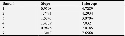
Figure 2. Example of data applied in the model.
2.3. Methods of Land Cover Change Detection
2.3.1. Vegetation Indices
Vegetation indices are calculable measurements indicating the strength of vegetation (Campbell, 1987). They show better sensitivity than individual spectral bands for the detection of biomass (Asrar, et al., 1984). The interest of these catalogs deceits in their usefulness in the analysis of remote sensing images; they organize notably a method for the detection of land use changes (multi-temporal data), the assessment of vegetative cover solidity, crop perception and crop yield prediction (Baret, 1986). In the area of thematic mapping, the interest of most of these indices lies in the improvement of classifications (Asrar, et al., 1984; Bariou, et al., 1985a, 1985b; Qi, et al., 1991; McNairn, Protz, 1993). In this study, NDVI index was used in order to monitor vegetation cover changes during different time periods. Normalized Difference Vegetation Index (NDVI) is the most widely used vegetation index to discriminate healthy vegetation from others or from non-vegetated areas (Manandhar, et al., 2009).
NDVI represents the ratio between the red (RED) and near-infrared spectrum (NIR) (Equation 1) and was first used by (Rouse et al. in 1973). Healthy plants absorb most of the visible light and reflect the large amount of the far-red and near-infrared light (Fluor Cam PAR, 2014.). It is obtained from the Equation 1. Theoretically, the values of this index will vary within the range of -1 to 1. The research within this study showed that the values of NDVI index for vegetation are within the range between 0.3 and 0.7; the values above 0.6 indicated the existence of solid vegetation.
NDVI (1)
Change detection with the use of the vegetation indices included the expert classification with the help of vegetation indices for the 8-year period, between 2000 and 2008. The spectral signatures of the deciduous trees, coniferous trees, artificial objects and water areas have been extracted in the region and such spectral signatures were applied to the given area.
2.3.2. Crop Production Model
Table 4. Means and standard deviations of reported and simulated yields.
Crop
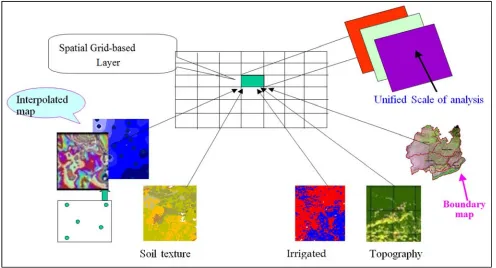
District Attock Average Yield (2000-2008)
Area in "000" Hectares Production in "000" Tonnes
Mean SD Mean SD
---tons/ha
---Wheat 145.411 12.67 202.78 79.04
Rice N. G N. G N. G N. G
Maize 17.922 1.84 17.71 5.67
Bajra 5.08 1.02 1.75 0.41
Jowar 17.97 3.80 7.72 3.46
Barley 2.17 0.58 1.72 0.55
Sugarcane 0.17 0.06 7.92 0.32
Cotton 00 00 00 00
Sunn Hemp 10.8 5.98 4.25 2.37
Jute N. G N. G N. G N. G
Tobacco 95.66 25.27 207.37 77.60
Guarseed 218.44 194.02 124.87 113.63
This table is based on the data detached by unsupervised classification through MODIS satellite Imagery 2000-2008 of Attock District.
Figure 3. Example of Average Yield District Attock (2000-2008).
Table 5. Means and standard deviations of reported and simulated yields.
Crop
District Rawalpindi Average Yield (2000-2008)
Area in "000" Hectares Production in "000" Tonnes
Mean SD Mean SD
---tons/ha
---Wheat 112.47 12.67 168.93 54.84
Rice N. G N. G N. G N. G
Maize 49.32 1.667 51.71 1.66
Bajra 9.68 1.02 3.475 0.69
Jowar 33.87 3.71 15.38 2.47
Barley 0.50 0. 07 0.45 0.11
Sugarcane N. G N. G N. G N. G
Cotton N. G N. G N. G N. G
Sun hemp 12.5 5.68 5.75 2.60
Jute N. G N. G N. G N. G
Tobacco N. G N. G N. G N. G
Guarseed 4.62 11.55 3.75 5.97
44 Muhammad Zubair Iqbal and Muhammad Javed Iqbal: Land Use Detection Using Remote Sensing and GIS (A Case Study of Rawalpindi Division)
Figure 4. Example of Average Yield District Rawalpindi (2000-2008).
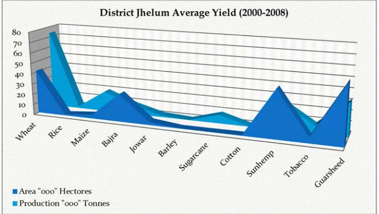
Table 6. Means and standard deviations of reported and simulated yields.
Crop
District Jhelum Average Yield (2000-2008)
Area in "000" Hectares Production in "000" Tonnes
Mean SD Mean SD
---tons/ha---
Wheat 41.31 4.18 73.73 27.15
Rice 1.15 0.25 1.8 0.39
Maize 3.66 0.77 19.33 8.92
Bajra 26.62 1.61 8.96 1.61
Jowar 3.31 0.39 1.78 0.25
Barley 0.12 0. 07 0.085 0.037
Sugarcane 0.2 2.96 8.33 0.43
Cotton 0.4 5.93 0.38 0.035
Sun Hemp 45.25 18.71 25.75 11.68
Jute N. G N. G N. G N. G
Tobacco 5.87 0.35 7.75 0.71
Guarseed 56.0 30.35 32.12 16.37
This table is based on the data detached by unsupervised classification through MODIS satellite Imagery 2000-2008 of Jhelum District.
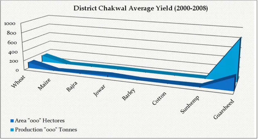
Table 7. Means and standard deviations of reported and simulated yields.
Crop
District Chakwal Average Yield (2000-2008)
Area in "000" Hectares Production in "000" Tonnes
Mean SD Mean SD
---tons/ha---
Wheat 126.47 7.43 141.9 51.16
Rice N. G N. G N. G N. G
Maize 0.7 0.30 0.77 0.31
Bajra 18.42 1.27 6.18 0.72
Jowar 31.42 1.31 9.15 1.62
Barley 1.03 0.25 0.81 0.11
Sugarcane 00 00 00 00
Cotton 0.25 0.20 0.23 0.19
Sun Hemp 10.62 5.42 4.8 3.04
Jute N. G N. G N. G N. G
Tobacco N. G N. G N. G N. G
Guarseed 265.68 328.63 860.5 130.93
This table is based on the data detached by unsupervised classification through MODIS satellite Imagery 2000-2008 of Chakwal District.
Figure 6. Example of Average Yield District Chakwal (2000-2008).
2.4. Land Use / Land Cover Change Detection Modeling
The success of change detection from imagery will depend on all, the image pre-processing, classification procedures and the nature of the change involved. If the nature of change within a particular scene is either rapid or at a scale appropriate to the imagery collected then change should be relatively easy to detect problems occurred only if the spatial change is slightly distributed and hence not obvious within an image pixel. (Milne, A. K., 1988).In the case of the study area chosen, field observation and measurements have shown that the change in land cover between the three dates was both marked and rapid.
46 Muhammad Zubair Iqbal and Muhammad Javed Iqbal: Land Use Detection Using Remote Sensing and GIS (A Case Study of Rawalpindi Division)
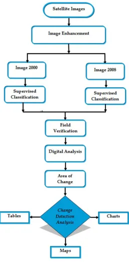
Figure 7. Flow Diagram.
2.5. Data Processing
Based on the idea that different feature types on the earth's surface have a different spectral reflectance and emittance properties, their recognition is carried out through the classification process. In a broad sense, image classification is defined as the process of categorizing all pixels in an image or raw remotely sensed raw satellite data to obtain a given set of labels or land cover themes (Lillesand, Keifer 1994).
Knowledge of both Remote Sensing and Geographic Information System (GIS) was used to generate the land
use/land cover maps of the periods in consideration (2000 and 2008). They were also used to do the following;
i.) To calculate the area in a square kilometer of each of the six classes of land use/land cover type.
ii.) To calculate the percentage change in the total area covered by the five different land use/land cover types.
iii.) To calculate the accuracy of the overall classification. iv.) To calculate the overall Co-efficient.
Table 8. Land use/land cover classification scheme and their general description.
Classes Description
Built Up Area Residential, Commercial, Industrial, Facilities and settlements
Barren Land Open Land and Non-Vegetated land
Forest Evergreen forest and Mixed forests with the higher density of trees.
Vegetation All Types of Agricultural Crops
Water Bodies Areas covered by dam’s water such as rivers, ponds, lagoons, dams and waterlogged areas.
Elsewhere the wide overviews of a cause - effect relationship. They are;
i.) Rate of change of land use/land covers (LULC) ii.) Land use/land covers change extent
The Image processing procedures, Image compositing, design of the classification, accuracy assessment, analysis of the land use/land cover subtleties as well as the assessment of the change between the different years under consideration (Austine O Nnaji, Njoku E Richard, and Peter C Chibuike march 2016).
2.6. Supervised Image Classification
The detection methods used in this study is based on the supervised classification. Change detection is based on the classification of all the image pixels from one time period in accordance with the pre-set number of classes, where the classes signify the suitable land cover class. Change detection is the most common approach (post-classification comparison) to detect the land use changes in terms of thematic classes (Al-Hassideh, et al., 2008, & Foody, 2002).
This is one of the methods which answers the question where and which changes have taken place. The two most basic types of classification methods are supervised and unsupervised classification. Both are machine learning approaches. Unsupervised methods use the specified number of classes and they mathematically recognize classes by measuring image pixels value differences. After that, those once classified classes need to be classified and grouped again in the way that presents results. In supervised classification, it is necessary to select several characteristic training samples from the image for each of the classes. After that computer examines the whole image and classifies pixels into one of the created classes.
Maximum possibility classification technique was performed using all spectral bands in each satellite image (Langford, Bell, 1997). In this study, the post-classification was used, which as a change detection method that represents an independent classification of the images from two different time periods (Figure 8 & 10), and then the comparison of the results.
48 Muhammad Zubair Iqbal and Muhammad Javed Iqbal: Land Use Detection Using Remote Sensing and GIS (A Case Study of Rawalpindi Division)
Table 9. Land use/cover.
Class Name Area (Sq. km)
Built-up Area 402
Vegetation 3731
Forest 2820
Water Channel 416
Barren Land 14928
Figure 9. Land use/cover.
Table 10. Land use/cover.
Class Name Area (Sq. km)
Built-up Area 578
Vegetation 4069
Forest 2113
Water Channel 400
Barren Land 15181
Figure 11. Land use/cover.
3. Land Use / Cover Status
Figure 8 & 10 shows land use/cover image after supervised classification. These images provide the pattern of land use/cover of the study area. The brown color represents settlements, green color vegetation, dark green color forest, blue color water and lite medium sand color shows barren land. Both land cover class maps were compared with reference data, which was prepared by ground truth, sample points and google earth. Overall classification accuracy of the study area was more than 90% for all two dates.
4. Assessment of Significant Change
Classification maps were generated for all of the eight years shown in figure 7 & 9 and the individual class area and change statistics are summarized in table 7 & 8. In 2000 the urban area covered 402 km² (2.00%), but by 2008 it had increased to approximately 578 km² (3.00%). The agricultural area initially increased from 3731 km² (17.00%) in 2000 to 4069 km² (18%) by 2008. The forested area decreased from 2000, 2820 km² (12.00%) to 2113 km²
(9.00%) by 2008. The barren area was 14928 km² (67.00%) in 2000, in 2008 had increased 15181 km² (68.00%). The inland water area remains approximately similar from 2000 416 km² (2.00%) to 400 km² (2.00%) by 2008. Although the extent of this change from year to year due to varying precipitation and temperature and although variation is also likely due to classification errors, because of the high classification accuracy for water small fluctuations in water are believed to be related to different water levels.
The results indicate that from 2000 to 2008 agriculture areas has minor change but a colossal change is in the forest areas. In the same time period built-up area was the increase but the barren land area was approximately remain same. Maximum extension of settlements was in agriculture area agriculture area was converted into settlements. The maximum stable class was water body, where areas were stable from 2000 to 2008.
50 Muhammad Zubair Iqbal and Muhammad Javed Iqbal: Land Use Detection Using Remote Sensing and GIS (A Case Study of Rawalpindi Division)
a growth in agricultural outputs like food and fibers to positively impact on the country’s economy and human well-being. As well as the huge decrease in forest land there has also been a quite considerable increase in urban settlements. Such changes require rapid adjustments to land management in order to avoid crises in the category of food and climate effect. From a socio-economic point of view, this means not
only a loss of ecosystem services but also a decline of earn money and cultural values, not to mention a subsequent reduction of income from tourism. A significance of this is to make protected areas some of the few remaining zones where fuel wood, rich pastures, and game resources are left and so they attract more and more legal activities.
Figure 12. Spatio-temporal patterns of land use/Land cover changes.
5. Conclusion
The objective of this study was to study the urban spread and its impact on agriculture land and forest in Rawalpindi division and to examine the capabilities of integrating remote sensing and GIS in studying the spatial distribution and extent of urbanization. It was found that integrating visual interpretation with supervised classification led to increasing in the overall accuracy. The study area has experienced a very severe land cover change as a result of urbanization which resulted in the rapid population. A Considerable increase in urban settlements has taken place at the expense of the most fertile and forest land in the governorate. Integrating GIS and remote sensing provided valuable information on the nature of land cover changes especially the area and spatial distribution of different land cover changes.
The main causes of urbanization are the rapid population growth in addition to the internal. This problem needs to be seriously studied, through multi-dimensional fields including socioeconomic, in order to preserve the precious and limited agricultural land and increase food production.
References
[1] Singh R B and Dilip Kumar (2012). ”Remote sensing and GIS for land use/cover mapping and integrated land management: case from the middle Ganga plain” Journal of Front. Earth Sci. (springer), Vol. 6 (2).
[2] Tricart E. Revista Brasileira de Geomorfologia Ano 8, nº 2 (2007), 1977.
[3] Boori M. S., Choudhary K., Kupriyanov A., Kovelskiy V. Urbanization data of Samara City, Russia. Data in Brief. 6 (2016).
[4] Xavierdasilva, J. et al. Índices de geodiversidade: aplicações de SGI em estudos de biodiversidade. In: Garay, I.; Dias, B. F. S. (Orgs.). Conservação da biodiversidade em ecossistemas tropicais: avanços con-ceituais e revisão novas metodologias de avaliação e monitoramento. Rio de Janeiro, Vozes, 2001, 299-316.
[5] Boori M. S., Vozenilek V. Land-cover disturbances due to tourism in Jeseniky mountain region: A remote sensing and GIS-based approach. SPIE Remote Sensing 2014; 9245, 92450T: 01-11. Doi:10.1117/12.2065112.
[6] Padgett J., Tapia C. "Sustainability of Natural Hazard Risk Mitigation: Life Cycle Analysis of Environmental Indicators for Bridge Infrastructure." J. Infrastruct. Syst., 2013; 19 (4), 395-408.
[7] Rogan J., Eastman J. R., Turner II B. L. Quantifying uncertainty and confusion in land change analyses: a case study from central Mexico using MODIS data. Vol. 52/5, pp 543-570, 2015.
[9] Andy Berman, Bambang Hendro Sarmiento, Sri Nuryani Hidayah Utami and Totok Gunawan (2013). “The Combination Of Land Resource Evaluation Approach And Gis Application To Determine Prime Commodities For Agricultural Land Use Planning At Developed Area – A Case Study Of Central Kalimantan Province, Indonesia". ARPN Journal of Agricultural and Biological Science Vol. 8, (12) pp. 771-784. Note that the journal title, volume number, and issue number are set in italics.
[10] Spatiotemporal analysis of land use/land cover changes, Imo State, Nigeria Austine Nnaji, Njoku E Richard and Peter C Chibuike March 2016.
[11] U.S. Department of the Interior U.S. Geological Survey. [12] Campbell, J. B. 1987. Introduction to Remote Sensing. [13] Asrar, G., Fuchs, M., Kanemasu, E. T., Hatfield, J. L. 1984. [14] Baret, F. 1986. Contribution au suiviradiométrique decultures
de céréales.
[15] McNairn, H., Protz, R. 1993. Mapping corn residue cover on agricultural fields in Oxford County, Ontario, using Thematic Mapper.
[16] Manandhar, R., Odeh, I. O. A., Ancev, T. 2009. Improving the Accuracy of Land Use and Land Cover.
[17] Rouse 1973, Classification of Landsat Data using Post-classification Enhancement.
[18] Fluor Cam PAR, 2014. Absorptivity Module & NDVI Measurement Instruction Manual, product PSI, spoil.
[19] Satya Priya and Ryosuke Shibasaki 2002 National Spatial Crop Yield Simulation Using GIS-Based Crop Production Model.
[20] Milne, A. K., 1988. Change detection analysis using Landsat imagery a review of methodology. In: Proceedings of IGARSS, 88 Symposium, Edinburgh, Scotland, 13-16 September 1988. pp. 541-544.
[21] Lillesand, T. M. & Keifer, R. W. 1994, Remote Sensing and Image Interpretation. Al-Hassidic, Bill R. 2008. Land Cover Changes In The Region Of Rostock - Can Remote Sensing And Gis Help To Verify And Consolidate Official Census Data. Rostock University, Chair of Geodes.
[22] Foody, G. M. 2002. Status of land cover classification accuracy assessment. Remote Sensing of Environment 80, 1, 185-201.