Computation of ontology resemblance coefficients for improving semantic interoperability

*

Corresponding author Received December 10, 2012

1 Available online at http://scik.org

Engineering Mathematics Letters, 2 (2013), No. 1, 1-19 ISSN 2049-9337

COMPUTATION OF ONTOLOGY RESEMBLANCE COEFFICIENTS

FOR IMPROVING SEMANTIC INTEROPERABILITY

LAMBRINI SEREMETI1, IOANNIS KOUGIAS2,*

1

Faculty of Science and Technology, Hellenic Open University, Patras, Greece

2

Department of Telecommunication Systems and Networks, Technological Educational Institute of Messolonghi, Greece

Abstract: In open and dynamic environments, where various heterogeneous agents need to communicate, a shared ontology that explicitly and formally describes the whole domain of interest, or an alignment that provides semantically related entities among distinct ontologies, can be employed. The former case is infeasible, because a unique conceptual view of a domain is not widely accepted. Hence, the case, usually adopted, is the latter, where independently developed heterogeneous ontologies exist. A challenging issue is how an agent, charged with the task of carrying out the alignment, should select a suitable execution of matchers, to establish correspondences between ontology entities, in the fastest and most efficient way. A solution to this challenge is to use metrics for estimating the resemblance of a given pair of ontologies. To this end, we propose two metrics, as similarity coefficients, to estimate the lexical or structural resemblance of a given pair of ontologies.

Keywords: ontologies; heterogeneity; ontology alignment; similarity metrics; semantic interoperability.

1. Introduction

The ability to communicate is one of the key capabilities of an agent (whether human,

or machine) within a multi-agent environment. The entities in these smart

environments can maintain their own semantic descriptions by using ontologies, which

are formal knowledge representation models [6]. Unfortunately, the variety of ways

that a domain can be conceptualized, results in the creation of heterogeneous

ontologies with contradicting, or overlapping parts. The heterogeneity, at the ontology

level, can mainly occur because of two reasons: (1) different ontologies could use

different terminologies to describe the same domain of interest, and (2) even if two

ontologies use the same names/labels for their entities, their corresponding structure

can be different. Consequently, in order to achieve successful communication within

such environments, where ontologies are used, it is necessary to bring them into a

mutual agreement, that is, to align them, by establishing semantically related entities

between the two ontologies [3]. Various methods and tools for assisting the process of

ontology alignment have been developed. Based on our experience [9] with small and

medium size ontologies which are characterized by limited hierarchy and not

well-defined terminology, we have observed that the proposed algorithms

(lexical-based, structure-based, constraint-based, instance-based) and strategies

(execution of a single alignment algorithm, a parallel, or a sequential execution of

ontology alignment algorithms) do not perform well in the case of limited hierarchy

structure of the involved ontologies, or absence of constraints, or entity labels being

tightly oriented towards the creator’s view of the domain and not towards a general,

common and agreed-upon vocabulary of the domain.

The usual practice in an alignment problem is to select a suitable alignment tool,

import the ontologies in question and finally accept, or reject some of the suggested

correspondences that the tool has produced. This is significantly far from getting

quickly the best results, because it depends on the selection of the tool, its collection of

matchers (alignment algorithms), their composition in execution (parallel, or

kind of heterogeneity they introduce, etc. So, one of the challenging issues in ontology

alignment in multi-agent environments, when good results in real-time are needed, is to

estimate whether the heterogeneity of the ontologies to be aligned, is mainly lexical, or

structural.

The solution we propose to this challenging issue is to assess the lexical and the

structural similarity of the pair of ontologies to be aligned and depending on these

measures, decide whether to apply a string-based, or a structure-based alignment

algorithm.

The rest of this paper is organized as follows: Sections 2 and 3 briefly introduce related

work in ontology alignment and various similarity metrics that are used by different

matchers, in order to compare entities of a given pair of ontologies from different

perspectives. Section 4 presents the proposed similarity measures as coefficients able

to estimate two ontologies’ resemblance and Section 5 concludes with future work.

2. Related Work on Ontology Alignment

Many researchers have investigated the problem of ontology alignment, mostly by

proposing several ontology alignment tools and matchers (or matching algorithms) [4],

[5], [7], which exploit various types of information in ontologies, that is, entity labels,

taxonomy structures, constraints and entities’ instances. These tools can be classified

into two large categories: those that make use of a single matcher in order to calculate

similarities between ontology entities and those which use a family of parallel or

sequential matchers in composition. In the latter category, the similarity between two

ontology entities is finally computed by a composite method, such as a weighted

aggregation of the similarities obtained by each matcher separately.

A challenging issue while applying these methods consists of deciding whether a

single matcher, or a combination of different matchers, performs better and in what

cases, that is, for which kind of ontologies in question. Hence, given a specific pair

matcher should be used. Based on this consideration, we propose the calculation,

during a pre-alignment step, of two similarity coefficients, which estimate whether the

resemblance of the ontologies in question is mainly lexical, or structural. Then,

depending on their values, an agent who is charged with the task of the alignment

process, can select the execution of suitable matchers, in order to establish

correspondences between ontology entities, in a more effective and efficient way.

3. Related Work on Similarity Metrics

Considerable work has been made on metrics for measuring the degree of similarity

between two entities of the ontologies to be aligned [2], [5], [8]. These metrics are

functions that map a pair of entities of a given pair of ontologies to a value between 0

and 1, and they can be mainly classified into string-based and structure-based metrics.

The purpose of these measures is to have a means to calculate lexical or structural

similarity, respectively, between the entities of the given ontologies.

Our goal in presenting the new measures is to study the resemblance between

ontologies in question, instead of studying the detailed relationship between entities of

the given pair of ontologies, as do the metrics proposed in the literature. Although

these metrics can provide good results regarding the similarity between entities, that is,

at the entities’ level, they are inappropriate at the ontology level. Ontologies used in

multi-agent environments require processing in real-time, so the complexity of the

classical metrics used at the ontology level, should be very low, leading to a fast

estimation of ontologies’ resemblance. As far as we know, such a kind of measures is

used by the RiMOM ontology alignment multi-strategy [10], in order to enhance the

alignment process. In comparison with RiMOM’s metrics, our proposed measures

appear to be more accurate, as we demonstrate later in section 4.

4. Similarity Coefficients

An agent charged with the task of the alignment process must be aware of the

coefficients for ontology resemblance (structural, or lexical). These coefficients are

used during a pre-alignment process, in order to select the suitable family of matchers,

as well as the way of composing them. Their values fall into the range of the closed

interval [0,1] . The first of the similarity coefficients examines the relative structure of

the two ontologies, based on the comparison of the lengths of all paths leading from

the root of each ontology to each of its leaves. The second one, after discovering

concepts with identical labels in both ontologies, considers the relative proximity of

these common concepts, inside each one of the ontologies to be aligned.

4.1 Definition of Similarity Coefficients

We define the Structural Similarity Coefficient, denoted by(O O₁, ₂), which is a similarity metrics at an ontology level (as opposed to an entity level), with values that

range from 0 to 1 . The Structural Similarity Coefficient describes the similarity

between two ontologies globally (as opposed to local structural similarities between

ontology entities), based on their structural resemblance. In order to compute it, one

has to follow the constructive procedure described below:

4.1.1 Definition of the Structural Similarity Coefficient

Given two ontologies O₁andO₂, calculate the vectors l₁, l₂ having as elements the lengths of all the paths from the root of each ontology, to all its leaves, i.e.,





1 11,12,..., ,...1i

l  l l l , with l_1i  length of the path from the root of ontology O₁ to its

th

i leaf, i1, 2,..., # leaves of ontology O₁

2 21, 22,..., 2j,...

l  l l l _ with l_2j  length of the path from root of ontology O2 to its

th

j leaf, j1, 2,..., # leaves of ontology O₂

greatest dimension and by completing the other vector with leading zeros. Both vectors

a, t, have dimension L.

If | | |l_i  l_j|, i j, {1, 2} and i j, then al_i, t  0,lj, with the dimension of 0 being equal to Lmin{| |,|l₁ l₂|}.

Now compute a square LxLmatrixC, with elementsc_ij |a_it_j|, i j, 1, 2,...,L.

Then, create two new vectors r ands, by appropriately reordering the vectors a

and t, as explained hereafter.

Let us consider two sets B and T with cardinalities equal to L and leti, i,

1, 2,...,

i L, denote their respective elements. Consider the bipartite graph having as

nodes the elements of the sets B and T and containing all possible edges between

respective elements of the two sets. The edge linking_i, to _j i j, 1, 2,...,L, has a

weight equal to c_ij |a_it_j|. One can then always find a square matrix X with

dimensions LxL having elements x_ij , ,i j1, 2,...,L , such that the following

relations hold:

1.  i 1, 2,...,L,

1

1

L

ij j

x







2.  j 1, 2,...,L,

1

1

L

ij i

x







3. i j, 1, 2,..., ,L x_ij 0

4.

1 1

L L

ij ij

i j

c x

 



is minimized

It can be proven that such elements x_ij, ,i j1, 2,...,L, exist and take either the value

while the jth element of the reordering s is s_j t_j. The structural similarity

between the two ontologies is finally calculated as the cosine of the angle between the

vectors r and s:

1 1 2 2 2 1 1 . ( , ) || || . || || L i i i L L i i i i r s r s O O

r s _{r s}

 

 

 



 

. (1)

We define the Lexical Similarity Coefficient, at an ontology level, with values ranging

from 0 to 1. In order to calculate the Lexical Similarity Coefficient, we consider two

factors. The first factor is based on the number of concepts/classes having the same

label in both ontologies (inter-ontology factor), while the second one takes into

account the relative proximity that these common concepts have among them, inside

each one of the ontologies (intra-ontology factor).

4.1.2 Definition of the Lexical Similarity Coefficient

Given two ontologies O_i and O_j, ,i j1, 2, i j , with a number of cc pairs of

concepts with the same label, that is, ( ₁Oi, ₁Oj),

2 2

( Oi, Oj),…,₍ Oi_, Oj₎

k k

  , ,i j1, 2,

i j , k 1, 2,...,cc, respectively, the Lexical Similarity Coefficient is calculated as:

 

 

 

 

1

1

max( , )

( , )

max(# , # )

[

]

j i j i O O

cc _{k k}

O O

k _{k k}

i j i j O O conceptsofO conceptsofO             



, (2)

, 1, 2

i j , i j, where the term

 

Oi

k

  ranks concept Oi

k

 of ontology O_i, by taking

into account how far, in terms of number of edges, the remaining common concepts

,

i

O

p p k

  are from concept Oi

k

 in ontology O_iand is given by

 



    







_{ }

_

_







 





1 2 1 1 , ,

1 1 1 ...

1 1

, ,

... 1 1 1 1 ,

1 1

i i

i i i i

i i

i i

O O

k k

O O O O

k k k k

O O

k m _O m k m _O m

k k

d n d n

cc cc

d n d n

cc cc





 























 





                

where



1



1 ( 1)sgn[( 1) , ]

i i

O O

k cc d k n

       1

, (4)

with , ( 0  1 ) a constant added to the rank of common concept Oi

k

 , due to its

lexical similarity to concept Oj, , 1, 2,

k i j i j

   and where we define:

1

n to be the 1-neighborhood of concept Oi

k

 , containing all common concepts

,

i

O

p p k

  , that are within a distance of exactly one edge from Oi

k

 in O_i,

2

n to be the 2-neighborhood of concept Oi

k

 , containing all common concepts

,

i

O

p p k

  , that are within a distance of exactly two edges from Oi

k

 in Oi,

…

…

m

n to be the m-neighborhood of concept Oi

k

 , containing all common concepts

,

i

O

p p k

  , that are within a distance of exactly m edges from Oi

k

 in O_i,



nm1



O to be the remote-neighborhood of concept Oi

k

 , containing all common

concepts Oi,

p p k

  , that are within a distance of more than m edges from Oi

k

 in

i O .

Then,



Oi,



, 1, 2,...,

k q

d  n q m, denotes the number of common concepts Oi,

p p k

 

that are within a distance of exactly qedges from Oi

k

 in O_iand



Oi, ( ₁)



k m

d  O n _

denotes the number of common concepts Oi,

p p k

  , within a distance of more than

m edges from Oi

k

 in O_i.

1

The signum function is defined as:

1 0

sgn( ) 0 0

1 0

if x

x if x

1

1

2  is a forgetting factor, penalizing more severely the common concepts

,

i

O

p p k

  that are more distant from Oi

k

 in O_i (in more distant neighborhoods).

4.2 Implementation of Similarity Coefficients

The idea behind the Structural Similarity Coefficient, is to compare the structure of the

two ontologies, based on the minimization of the sum of the absolute values of the

differences between the lengths of all the respective pairs of paths belonging to the two

ontologies; these paths lead from the root of each ontology to each of its leaves.

In order to count the lengths of the paths, we can use a graph traversal algorithm like

DFS (Depth First Search) together with a counter, initialized at zero, augmented by

one each time an edge is found, decreased by one each time that backtracking is

considered and memorized in a stack each time a leaf (no descendants) is encountered.

DFS is effective enough, of complexity (V2) when a representation with adjacency matrices is used and  (V E) when a representation with adjacency lists is used,

where V is the number of the graph vertices and E is the number of the graph

edges.

The vectors l₁, l₂ having as elements the lengths of all the paths of the ontologies thus obtained, may have different dimensions. That is why we add leading zeros to the

vector with the lower dimension, in order to compensate this difference in dimensions

(these zeros can be considered to correspond to the missing paths of one of the

ontologies with respect to the other). The vectors a and t are thus obtained. We

have now established a correspondence between the paths of one of the ontologies and

the respective paths of the second one. In the aim to minimize the sum of the absolute

values of the differences of the lengths of the corresponding pairs of paths, we need to

reorder the vectors a and t into new vectors r and s, respectively.

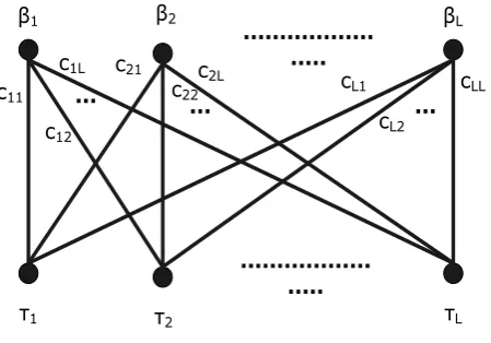
In order to achieve this, we reformulate the problem, as a linear assignment problem.

sets B and Tof cardinalityL, as seen in Figure 1. We consider that the edge linking

i

 to _j, i j, 1, 2,...,L, has a weight equal to c_ij |a_it_j| (i.e. the absolute value

of the difference of the lengths of the respective paths).

β1 βL

τ1 τ₂ τL

... ... ...

... c11

c12

c1L c21

c22

c2L _c

L1

cL2

cLL

... _{... ...}

β2

Figure 1. The bipartite graph between the elements of the sets Band T

The matrix C corresponds to a weight function C BxT: R. In order to maximize

the resemblance between the structures of the two ontologies, we need to minimize the

sum of the absolute values of the differences of lengths between respective paths, that

is, referring to Figure 1, we need to find a bijectionf B: T, such that the cost function

1 L

ij i

c





is minimized, with f(_i)_j being the image of _i under the bijection f . But,

this is the formal definition of the linear assignment problem. The assignment problem

is a special case of the transportation problem, which is a special case of the minimum

cost flow problem, which in turn is a special case of the linear problem. It is thus

possible to solve the minimization problem that we have, by using the simplex

algorithm (very effective in practice, generally taking 2 to 3 times the number of

equality constraints iterations at most and converging in expected polynomial time for

certain distributions of random inputs), or more specialized algorithms, like the

a matrix X with dimensionsLxL, having elements x_ij, i j, 1, 2,...,L, that minimizes

the objective function 1 1 L L ij ij i j c x  



, subject to the following constraints:

1.  i 1, 2,...,L,

1 1 L ij j x  



, that is, each element of the set B is assigned to

exactly one element of the set T

2.  j 1, 2,...,L,

1 1 L ij i x  



, that is, each element of the set T is assigned to exactly

one element of the set B

Both the above mentioned constraints are due to the bijection f that we are

searching.

3. i j, 0,1,..., ,L x_ij0

The variablesx_ij , i j, 1, 2,...,L represent the assignment (or not) of _i to_j ,

, 1, 2,...,

i j L, taking the value 1 if the assignment is done and taking the value 0

otherwise. The vectors r and s are obtained by appropriately reordering the vectors

a and t with the help of the matrixX, which is obtained as the solution of the

simplex algorithm. The matrix X has only one non zero element in each of its rows

and in each of its columns and this non zero element has a value of 1. If for some

1

ij

x  , then the ith element of the reordering r is r_i a_i, while the jth element of

the reordering s is s_j t_j.

Finally, the structural similarity between the two ontologies is calculated as the cosine

of the angle between the vectors r and s:

1 1 2 2 2 1 1

.

(

,

)

|| || . || ||

L i i i L L i i i i

r s

r s

O O

r

s

r

s



  







As a more time efficient alternative, the reordered vectors r and s can be obtained

by simply sorting the vectors a and t with a Vlog( )V algorithm like quicksort

and then taking pairs of values which are at the same positions in the two sorted

vectors.

The idea behind the Lexical Similarity Coefficient is to initially rank each common

concept in both ontologies, based on the distance, in terms of the number of edges,

between this common concept and all the remaining common concepts, in each

ontology. Then, if a common concept is ranked equally in both ontologies, we assign

the value 1 for this pair of common concepts in the calculation of the Lexical

Similarity Coefficient, else, i.e., if a common concept is ranked differently in both

ontologies, we substract from the value of 1 , an amount which depends on the

difference of rankings.

In order to compute the Lexical Similarity Coefficient, firstly, the concepts/classes of

the two ontologies O₁and O₂are examined for the presence of same labels. After case normalization, diacritics suppression, blank normalization, link stripping, punctuation

elimination applied to both ontologies, a total string is formed from the labels of all

classes/concepts of ontology O₁. Then, each label of classes/concepts of ontology

2

O , is compared to this total string, by using a string matching algorithm, such as the

Boyer-Moore algorithm (( )w , with w the length of the total string in O₁).

In this way, corresponding pairs of same labels

1 2

1 1

( O, O ), 1 2

2 2

( O, O ),…,₍ O1_, O2_{), 1, 2,...,}

k k k cc

   are established and memorized, with

1 O k

 the label of a concept in O₁and O2 k

 the same label of the corresponding concept in

2 O .

For each label Oi

k

 ,i1, 2, k1, 2,...,cc , we then count the number of labels

,

i

O

p p k

  that are in the 1 , 2 ,...,  m neighborhoods of Oi

k

respectively. The remaining labels belong to the remote- neighborhoods O



n_m1



in

, 1, 2

i

O i . The quantities



Oi,



, 1, 2,..., , 1, 2, 1, 2,...,

k q

d  n k cc i q m , as well as



, ( 1) ,



1, 2,..., , 1, 2

i

O

k m

d  O n _ k cc i , can thus be computed.

Practically, we search for the labels Oi,

p p k

  in the 1-neighborhood (parent_of and

children_of Oi

k

 ) and in the 2-neighborhood (parent_of (parent_of), children_of

(parent_of) and children_of (children_of) Oi

k

 ). In this special case, the remaining

labels belong to O( )n₃ .

( , )

1

i

O k q

d n

cc 

 denotes the percentage of common labels i,

O p p k

  in a distance of

exactlyqedges from Oi

k

 , q1, 2,...,m, i.e. in its q-neighborhood in O ii, 1, 2.

In the ideal case of an infinite number of qneighborhoods, we would like to weight

the percentage of common labels Oi,

p p k

  in the n_q neighborhood of Oi

k

 ,

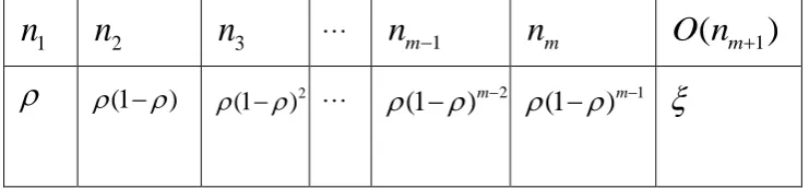
according to Table 1.

Table 1. Assignment of weights in the case of an infinite number of qneighborhoods

1

n

n

₂

n

₃ …

n

_q …



(1) 2

(1 )

  … 1

(1 )q



_



 _…

In practice, we restrain ourselves up to an m-neighborhood. In this case we have the

following assignment of weights of Table 2.

Table 2. Assignment of weights in the case restrained to an m-neighborhood

1

n

n

₂

n

₃ …

n

_m1

n

_m

O n

(

_m1

)



(1) 2

(1 )

  … 2

(1 )m



_



 1

(1 )m

We calculate in such a way that the sum of weights equals 1:









2 2 1

1 1 ... (1 )m (1 )m 1

 _{ } _ _ _{ } _  _ _  _{ }

from which, by using ₁ 2 _... 1 1

1

m

m 

  



 

    

 , we deduct that (1 )

m

   .

In order to have a decreasing series of weights, we impose  (1)m1, which

leads to the choice 1

2

 .

In the case where all Oi, p p k

  are in the 1-neighborhood of Oi

k

 in Oi, it is 1

i

O k

 

and thus ( Oi) 1

k

   . In all other cases, it is 0 Oi 1

k

 

   .

Concerning the complexity of the proposed Similarity Coefficients, the determining

factor, in the case of the Structural Similarity Coefficient, is the complexity of the

algorithm for resolving the assignment problem, while, in the case of the Lexical

Similarity Coefficient, the determining factor is the string matching problem. Since the

existing algorithms for solving these problems are efficient, exhibiting polynomial

running time, they confer polynomial computational complexity to the herein proposed

algorithms.

4.3 Examples of Similarity Coefficients

For the ontologies of Figure 2, we compute the Structural Similarity Coefficient as

1 2 _{2 2 2 2 2 2}

2 2 1 1 1 0 5

( , ) 0.9129,

6

2 1 1 2 1 0

O O

        

   

which means that they have very similar structure. The corresponding structure

similarity factor used in [10], in order to measure the structural similarity between two

Coefficient depicts more accurately the similarity of structure between the two

ontologies, which becomes apparent when flipping O₁ horizontally.

O1 O2

Figure 2. The ontologies of example 1

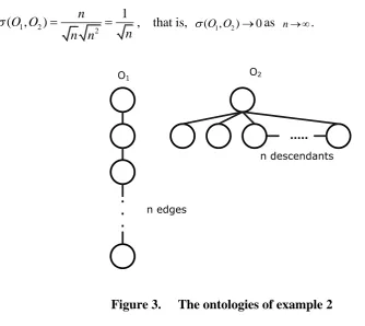
The Structural Similarity Coefficient for the ontologies of Figure 3 is calculated as

1 2 ₂

1

(O O, ) n

n n n

   , that is, (O O₁, ₂)0as n .

...

O1 O2

. . .

n descendants

n edges

Figure 3. The ontologies of example 2

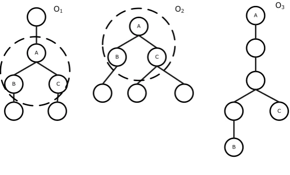
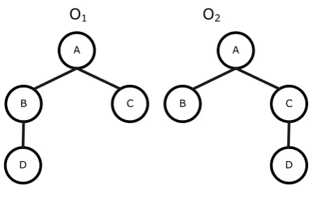
We consider now the ontologies of Figure 4 and compute the Lexical Similarity

Coefficient of pairs O₁and O₂and O₁andO₃, respectively, by choosing a0.8 and

0.6

A

B C

A

B C

O1 O2

A

C

B

O3

Figure 4. The ontologies of example 3

The ontologies O₁, O₂ and O₃ have common labels A, B and C . Thus, cc3

and we choose m2, limiting ourselves to 1 , 2 neighborhoods n n1, 2and O

 

n3 .

When computing the Lexical Similarity Coefficient between O₁and O₂, since each common concept distributes in the same way the remaining common concepts in its

neighborhoods, in both ontologies, it results that



₁, ₂



1 1 1 0.5 6

O O

     .

When comparing lexically O₁ to O₃, it is

 

_AO1

 =1,

   

1 1 _0.8 1 _{0.2 0.6} 1 _{0.2 0.6 0.4 0.884}

2 2

O O

B C

          

     

_AO2 _BO2 _CO2 _{0.8 1 0.2 0.4}2 _0.832

       

resulting in



1 3



(1 0.168) (1 0.0588) (1 0.0588)

, 0.4524

6 O O

        .

The lexical similarity factor proposed in [10], is computed to be equal to 0.5, for both

pairs of ontologies of the above presented example, taking into account that the three

ontology), but ignoring the fact that interrelations among them are not preserved the

same in O₃. In comparison, our Lexical Similarity Coefficient is more accurate. This is justified by the results obtained, where we calculate the lexical similarity between

1

O and O2to be equal to 0.5 (the interrelations among the common concepts A,

Band C are preserved in ontologies O₁ and O₂), while in the case of the lexical

similarity between O₁ and O₃, our coefficient is calculated to be less than 0.5, depicting the differences in the interrelations among common concepts in these

ontologies.

The detection of such differences in interrelations among common concepts is essential,

since it restricts the problem of polysemy (words that have multiple senses), occurring

when comparing ontology entities on the basis of their labels. Indeed, intuitively,

groups of common labels in both ontologies, are more probably referring to the same

concepts, while distant distinct common labels, may reflect homonyms and thus name

different concepts.

Another example is depicted in Figure 5, where the ontologies O₁ and O₂ have four common concepts.

A

B C

D

O1 O2

A

B C

D

Figure 5. The ontologies of example 4

Here, the common concepts Band Cdistribute differently the remaining common

concepts ( A , C and D for B and A , B and D for C ), while A and

ontologies. The result obtained is 



O O1, 2



0.9832. In opposition, the Lexical

Similarity Factor proposed in [10] is calculated to have a value of 1 for this pair of

ontologies, thus considering them as identical. The Lexical Similarity that we propose

is still more accurate, having a value of less than 1, due to the differences in

interrelations between the common concepts in the two ontologies. The exact amount

of the difference obtained, can be adjusted by a proper choice for the values of the

weighting coefficients a and .

5. Conclusion and future work

Ontology alignment tools have benefited a lot from the use of lexical and structural

similarity measures, in order to discover semantic correspondences between entities of

different ontologies. Though powerful metrics exist in literature, they have been

developed and purposed for a entities’ level comparison, instead of the herein proposed

metrics, which are suitable for a comparison at the ontology level. The ascertainment

that short size ontologies, as well as the particularities of other ontologies influence

adversely the performance of alignment tools that comprise a family of matchers and

that use metrics which are suitable for large-scale ontologies, motivated the suggestion

of two coefficients, which guide the selection of the right composition of available

matchers, in order for the alignment to be correct and fast.

Future work includes the implementation of these coefficients by using the Alignment

API 4.0 [1]. Then, experiments will be carried out with real-world ontologies and

finally standard metrics, such as precision (the percentage of correctly discovered

alignment in all discovered alignments) and recall (the percentage of correctly

discovered alignments in all correct alignments) will be used, to evaluate the alignment

REFERENCES

[1] J. David, J. Euzenat, F. Scharffe, C. T. dos Santos, The Alignment API 4.0, Semantic Web Journal 2 (2010) 3-10.

[2] D. Dhyani, M. W. Keong, S. Bhowmick, A survey of web metrics, aCM Computing Surveys 34 (2002) 469-503.

[3] M. Ehrig, Ontology Alignment: Bridging the semantic Gap, Springer, 2007.

[4] M. Ehrig, Y. Sure, FOAM – framework for ontology alignment and mapping; Results of the ontology alignment initiative, in: B. Ashpole, M. Ehrig, J. Euzenat, H. Stuckenschmidt (Eds.), CEUR Workshop on Integrating Ontologies Proceedings, 2005, pp. 72-76.

[5] J. Euzenat, P. Shvaiko, Ontology Matching, Springer-Verlag, Heidelberg (DE), 2007.

[6] T. Gruber, Towards Principles for the Design of Ontologies used for Knowledge Sharing, International Journal of Human-Computer Studies 43 (1995) 907-928.

[7] W. Hu, Y. Qu, G. Cheng, Matching large ontologies: A divide-and-conquer approach, Data & Knowledge Engineering 67 (2008) 140-160.

[8] R. Ichise, An analysis of multiple measures for ontology mapping problem, International Journal of Semantic Computing 4 (2010) 103-122.

[9] A. Kameas, L. Seremeti, Ontology-based knowledge management in NGAIEs, in: T. Heinroth, W. Minker (Eds.), Next Generation Intelligent Environments: Ambient Adaptive Systems, Springer, 2011, pp. 85-126.