Application of Real Ant Colony
Optimization Algorithm to Solve
Space and Time Fractional Heat
Conduction Inverse Problem
ITC 2/46
Journal of Information Technology and Control
Vol. 46 / No. 2 / 2017 pp. 171-182
DOI 10.5755/j01.itc.46.2.17298 © Kaunas University of Technology
Application of Real Ant Colony Optimization Algorithm to Solve Space and Time Fractional Heat Conduction Inverse Problem
Received 2016/12/20 Accepted after revision 2017/04/05
http://dx.doi.org/10.5755/j01.itc.46.2.17298
Corresponding author: [email protected]
Rafał Brociek, Damian Słota
Institute of Mathematics, Silesian University of Technology, Kaszubska 23, 44-100 Gliwice, Poland
This paper describes the method of solution of the space fractional and 2D time fractional heat conduction inverse problem. In this paper the authors consider two models – 1D space fractional heat conduction equation and 2D time fractional heat conduction equation with the initial-boundary conditions. To solve the inverse heat conduction problem, a functional defining the error of approximate solution must be minimized. To minimize this functional the Real Ant Colony Optimization (ACO) algorithm was used. In order to reduce the computa-tional time, the calculations were performed in a parallel (multi-threaded) way. The paper presents examples to illustrate the accuracy and stability of the presented algorithm.
KEYWORDS: Ant Colony Optimization Algorithm, Inverse Problem, Identification, Time Fractional Heat Conduction Equation, Space Fractional Heat Conduction Equation.
Introduction
Inverse problems are very important issues in sci-ence, they have a wide application in signal process-ing, communication theory, physics and many other fields of engineering. In this paper the authors con-sider the space and time fractional heat conduction inverse problem which consists in reconstructing the boundary condition in the fractional heat conduction models, basing on the temperature measurements. In
papers [13-15] the heat conduction inverse problems with the classical derivative are considered, whereas in articles [4-6] the fractional heat conduction in-verse problems are investigated.
Information Technology and Control 2017/2/46 172
10, 13-15, 21, 35, 40-43]. The most popular and effi-cient algorithms inspired by nature are the following algorithms: Ant Colony algorithms [12, 36], Artificial Bee Colony algorithm [16-18, 33] and Firefly algo-rithm [35]. In many cases these types of algoalgo-rithms provide better results than the conventional algo-rithms and, what is more, they are easy to implement. In case of optimization algorithms inspired by nature, another good feature of these algorithms is the fact that they do not need any requirements about mini-mized function, except the existence of the solution. Fractional calculus is very useful to model many var-ious types of physical and technical phenomena [8, 9, 11, 25, 26, 30, 34]. Application of fractional calculus can be found, for example, in electrical engineering [26], control theory [8, 11], mechanics [9]. In papers [30, 46] the authors consider the model of heat con-duction in ceramic and composite medium. The mod-els containing fractional derivative better describe the heat conduction process than the models with classical derivative. To solve fractional heat conduc-tion inverse problem, we need first to solve the direct problem. In paper [29] Murio presents the numerical method of solving the time fractional diffusion equa-tion with Dirichlet zero boundary condiequa-tions. Meer-schaert in paper [22] describes the numerical solu-tion of the space fracsolu-tional diffusion equasolu-tion with boundary condition of the first kind, and in paper [23] the authors present the finite difference method for two-dimensional fractional dispersion equation. In both papers, as the fractional derivative, the Rie-mann-Liouville derivative was used. In paper [3] the author presents the numerical solution of time frac-tional heat conduction equation with Neumann and Robin boundary conditions, and in paper [7] the au-thors consider the space fractional heat conduction equation with mixed boundary conditions.
In papers [27, 28] Murio deals with the inverse prob-lems of fractional order. Article [27] presents the solution of the time fractional inverse heat conduc-tion problem with Caputo fracconduc-tional derivative and in paper [28] the author reconstructs the heat flux in the fractional-diffusion heat conduction equation. Also in paper [24] the inverse diffusion problem is consid-ered. The problem consists in determining the spatial coefficient and the order of derivative. The authors prove that under certain conditions the solution of the problem is unique. The proof is done by transforming
the solution to the solution of the wave equation. In paper [38] the inverse problems of fractional order are considered. The inverse source problem is trans-formed into a first kind Volterra integral equation. Further, the authors use the boundary element meth-od and Tikhonov regularization to solve the Volterra integral equation of the first kind. Many other authors deal also with the various kinds of fractional inverse problems, see for example [2, 4-6, 20, 39, 44-46]. This paper describes an application of the parallel version of Real Ant Colony Optimization algorithm to reconstruct the heat flux at the boundary where the temperature distribution in measurement points is given. Two models are considered: 1D space fractional heat conduction equation and 2D time fractional heat conduction equation. To reconstruct the heat flux, a functional defining the error of approximate solution is minimized. In this purpose we use the Real Ant Colony Optimization algorithm, which inspiration is taken from the behavior of ant swarms, widely re-garded as the very intelligent communities, especially because of their tactics in search for the shortest path connecting the anthill with the source of food. In or-der to speed up the solving procedures we used the parallelization of the ant algorithm which significant-ly reduced the computation time. The direct problem in the proposed approach was solved by applying the implicit finite difference method [3, 7, 22, 23]. The pa-per also includes some examples illustrating the ac-curacy and stability of the presented procedures.
Formulation of the problem
We consider two mathematical models of fractional heat conduction equation.
Model I
First of all we introduce the following space fraction-al heat conduction equation
����(�,�)�� = �(�)�����(�,�)� (1)
� = { (�, �)� � � [�, �], � � [�, �∗) },
�(�, �) = �(�), � � [�, �], (2)
��(�)��(�,�)�� = �(�), � � (�, �∗), (3)
��(�)��(�,�)�� = ℎ(�)(�(�, �∗) � ��), � � (�, �∗), (4)
���(�,�)
��� =�(���)� � �
���� �(�, �)(� � �)�� ����� ��, (5)
�������(�,�,�)� = ��(�, �, �)�� �(�,�,�)
��� � ��(�, �, �)�� �(�,�,�)
��� � �(�, �, �) (6)
(1)
defined in region�� ��(�,�)
�� = �(�)
���(�,�)
��� (1)
� = { (�, �)� � � [�, �], � � [�, �∗) },
�(�, �) = �(�), � � [�, �], (2)
��(�)��(�,�)�� = �(�), � � (�, �∗), (3)
��(�)��(�,�)�� = ℎ(�)(�(�, �∗) � ��), � � (�, �∗), (4)
���(�,�)
��� =�(���)� � �
���� �(�, �)(� � �)�� ����� ��, (5)
�������(�,�,�)� = ��(�, �, �)�� �(�,�,�)
��� � ��(�, �, �)�� �(�,�,�)
where c, ����(�,�)�� = �(�)�����(�,�)� (1)
� = { (�, �)� � � [�, �], � � [�, �∗) },
�(�, �) = �(�), � � [�, �], (2)
��(�)��(�,�)�� = �(�), � � (�, �∗), (3)
��(�)��(�,�)�� = ℎ(�)(�(�, �∗) � ��), � � (�, �∗), (4)
���(�,�)
��� =�(���)� � �
���� �(�, �)(� � �)�� ����� ��, (5)
�������(�,�,�)� = ��(�, �, �)�� �(�,�,�)
��� � ��(�, �, �)�� �(�,�,�)
��� � �(�, �, �) (6)
, λ denote the specific heat, density and thermal conductivity, respectively. Equation (1) is completed with the initial condition
����(�,�)�� = �(�)�����(�,�)� (1)
� = { (�, �)� � � [�, �], � � [�, �∗) },
�(�, �) = �(�), � � [�, �], (2)
��(�)��(�,�)�� = �(�), � � (�, �∗), (3)
��(�)��(�,�)�� = ℎ(�)(�(�, �∗) � ��), � � (�, �∗), (4)
���(�,�)
��� =�(���)� � �
���� �(�, �)(� � �)�� ����� ��, (5)
�������(�,�,�)� = ��(�, �, �)�� �(�,�,�)
��� � ��(�, �, �)�� �(�,�,�)
��� � �(�, �, �) (6)
(2)
and the boundary conditions of the second and third kind
����(�,�)�� = �(�)�����(�,�)� (1)
� = { (�, �)� � � [�, �], � � [�, �∗) },
�(�, �) = �(�), � � [�, �], (2)
��(�)��(�,�)�� = �(�), � � (�, �∗), (3)
��(�)��(�,�)�� = ℎ(�)(�(�, �∗) � ��), � � (�, �∗), (4)
���(�,�) ��� =�(���)� � � ���� �(�, �)(� � �)����� ��, � � (5) �������(�,�,�)� = ��(�, �, �)�� �(�,�,�) ��� � ��(�, �, �) ���(�,�,�)
��� � �(�, �, �) (6) (3)
����(�,�)�� = �(�)�����(�,�)� (1)
� = { (�, �)� � ∈ [�, �], � ∈ [0, �∗) },
�(�, 0) = �(�), � ∈ [�, �], (2)
−�(�)��(�,�)�� = �(�), � ∈ (0, �∗), (3)
−�(�)��(�,�)�� = ℎ(�)(�(�, �∗)− ��), �∈(0, �∗), (4)
���(�,�)
��� =�(���)� � �
���� �(�, �)(� − �)�� ����� ��, (5)
�������(�,�,�)� = ��(�, �, �)�� �(�,�,�)
��� � ��(�, �, �)�� �(�,�,�)
��� � �(�, �, �) (6) (4)
where h is the heat transfer coefficient, q is the heat flux and
����(�,�)�� = �(�)�����(�,�)� (1)
� = { (�, �)� � ∈ [�, �], � ∈ [0, �∗) },
�(�, 0) = �(�), � ∈ [�, �], (2)
−�(�)��(�,�)�� = �(�), � ∈ (0, �∗), (3)
−�(�)��(�,�)�� = ℎ(�)(�(�, �∗)− ��), �∈(0, �∗), (4)
���(�,�)
��� =�(���)� � �
���� �(�, �)(� − �)�� ����� ��, (5)
�������(�,�,�)� = ��(�, �, �)�� �(�,�,�)
��� � ��(�, �, �)�� �(�,�,�)
��� � �(�, �, �) (6) denotes the ambient temperature. The space fractional derivative occurring in equation (1) is interpreted in the sense of the left-sided Rie-mann-Liouville derivative, which is defined by for-mula [34]:
����(�,�)�� = �(�)�����(�,�)� (1)
� = { (�, �)� � � [�, �], � � [�, �∗) },
�(�, �) = �(�), � � [�, �], (2)
−�(�)��(�,�)�� = �(�), � � (�, �∗), (3) −�(�)��(�,�)�� = ℎ(�)(�(�, �∗) − ��), � � (�, �∗), (4)
���(�,�)
��� =�(���)� � �
���� �(�, �)(�−�)�� ����� ��, (5)
�������(�,�,�)� = ��(�, �, �)�� �(�,�,�)
��� � ��(�, �, �)�� �(�,�,�)
��� � �(�, �, �) (6)
(5)
where Γ is the Gamma function, α∈(n –1, n]. In case of α∈(1, 2) equation (1) describes the phenomenon of super-diffusion, whereas for α =2 we get the differ-ential equation with classical derivative. In this paper we investigate α∈(1, 2).
Model II
Now, let us consider the 2D time fractional heat con-duction equation
����(�,�)�� = �(�)�����(�,�)� (1)
� = { (�, �)� � � [�, �], � � [�, �∗) },
�(�, �) = �(�), � � [�, �], (2)
��(�)��(�,�)�� = �(�), � � (�, �∗), (3)
��(�)��(�,�)�� = ℎ(�)(�(�, �∗) � ��), � � (�, �∗), (4)
���(�,�) ��� =�(���)� � � ���� �(�, �)(� � �)����� ��, � � (5) �������(�,�,�)� = ��(�, �, �) ���(�,�,�) ��� � ��(�, �, �) ���(�,�,�)
��� � �(�, �, �) (6)
����(�,�)�� = �(�)�����(�,�)� (1)
� = { (�, �)� � � [�, �], � � [�, �∗) },
�(�, �) = �(�), � � [�, �], (2)
��(�)��(�,�)�� = �(�), � � (�, �∗), (3)
��(�)��(�,�)�� = ℎ(�)(�(�, �∗) � ��), � � (�, �∗), (4)
���(�,�)
��� =�(���)� � �
���� �(�, �)(� � �)�� ����� ��, (5)
�������(�,�,�)� = ��(�, �, �)�� �(�,�,�)
��� � ��(�, �, �)�� �(�,�,�)
��� � �(�, �, �) (6)
(6)
defined in region
� � � (�� �� �)� � ∈ [�� ��]� � ∈ ��� ���� � ∈ [�� �∗]� ��� � �� �∗∈ ℝ� }, � � � (�� �� �)� � ∈ [�� ��]� � ∈ ��� ���� � ∈ [�� �∗]� ��� � �� �∗∈ ℝ� },
where α∈(0, 1), c is the specific heat, ����(�,�)�� = �(�)�����(�,�)� (1)
� = { (�, �)� � � [�, �], � � [�, �∗) },
�(�, �) = �(�), � � [�, �], (2)
��(�)��(�,�)�� = �(�), � � (�, �∗), (3)
��(�)��(�,�)�� = ℎ(�)(�(�, �∗) � ��), � � (�, �∗), (4)
���(�,�)
��� =�(���)� � �
���� �(�, �)(� � �)�� ����� ��, (5)
�������(�,�,�)� = ��(�, �, �)�� �(�,�,�)
��� � ��(�, �, �)�� �(�,�,�)
��� � �(�, �, �) (6)
is the density and λ1, λ2 > 0 for (x, y, t)∈D. To equation (6) we add the initial condition
�(�, �, �) = �(�, �), � � [�, ��], � � ��, ���, (7)
���(�, �, �) ��(�,�,�)�� = ��(�, �), � � [�, �∗], � � [�, ��], (8)
�����, ��, �� ����,����,��= ��(�, �), � � [�, �∗], � � [�, ��], (9)
���(�, �, �)��(�,�,�)�� = ℎ�(�, �)(�(�, �, �) � ��), � � [�, �∗], � � ��, ���, (10)
���(��, �, �)��(��,�,�)
�� = ℎ�(�, �)(�(��, �, �) � ��), � � [�, �∗], � � ��, ���, (11)
���(�,�)
��� =�(���)� � � ��(�,�)
��� (� � �)����� ��, �
� (12)
where Γ is the Gamma function and � � (� � �, �].
�(��, ��) = ����, � = �,�, � , ��, � = �,�, � , ��, (Model I) (13)
����, ��, ��� = ��(��)�, (��) = �,�, � , ��, � = �,�, � , ��, (Model II) (14)
�(ℎ) = ∑ ∑�� ����(ℎ) � ������, ���
��
��� (for Model I), (15)
�(ℎ�, ℎ�) = ∑�(��)��� ∑����� ��(��)�(ℎ�, ℎ�) � ��(��)���, (for Model II). (16)
(7)
and the Neumann (for y = 0, y = Ly) and Robin (for x = 0, x = Lx) boundary conditions:
�(�, �, 0) = �(�, �), � ∈ [0, ��], � ∈ �0, ���, (7)
−��(�, 0, �) ��(�,�,�)�� = ��(�, �), � ∈ [0, �∗], � ∈ [0, ��], (8)
−����, ��, �� ����,��,���� = ��(�, �), � ∈ [0, �∗], � ∈ [0, ��], (9)
−��(0, �, �)��(�,�,�)�� = ℎ�(�, �)(�(0, �, �) − ��), � ∈ [0, �∗], � ∈ �0, ���, (10)
−��(��, �, �)��(��,�,�)�� = ℎ�(�, �)(�(��, �, �) − ��), � ∈ [0, �∗], � ∈ �0, ���, (11)
���(�,�)
��� =�(���)� � � ��(�,�)
��� (� − �)����� ��, �
� (12)
where Γ is the Gamma function and � ∈ (� − �, �].
�(��, ��) = ����, � = �,�, � , ��, � = �,�, � , ��, (Model I) (13)
����, ��, ��� = ��(��)�, (��) = �,�, � , ��, � = �,�, � , ��, (Model II) (14)
�(ℎ) = ∑ ∑����� ���������(ℎ) − ������, (for Model I), (15)
�(ℎ�, ℎ�) = ∑��(��)��∑�������(��)�(ℎ�, ℎ�) − ��(��)���, (for Model II). (16) �(�, �, 0) = �(�, �), � ∈ [0, ��], � ∈ �0, ���, (7)
−��(�, 0, �) ��(�,�,�)�� = ��(�, �), � ∈ [0, �∗], � ∈ [0, ��], (8)
−����, ��, �� ����,��,���� = ��(�, �), � ∈ [0, �∗], � ∈ [0, ��], (9)
−��(0, �, �)��(�,�,�)�� = ℎ�(�, �)(�(0, �, �) − ��), � ∈ [0, �∗], � ∈ �0, ���, (10)
−��(��, �, �)��(��,�,�)
�� = ℎ�(�, �)(�(��, �, �) − ��), � ∈ [0, �∗], � ∈ �0, ���, (11)
���(�,�)
��� =�(���)� � � ��(�,�)
��� (� − �)����� ��, �
� (12)
where Γ is the Gamma function and � ∈ (� − �, �].
�(��, ��) = ����, � = �,�, � , ��, � = �,�, � , ��, (Model I) (13)
����, ��, ��� = ��(��)�, (��) = �,�, � , ��, � = �,�, � , ��, (Model II) (14)
�(ℎ) = ∑ ∑����� ���������(ℎ) − ������, (for Model I), (15)
�(ℎ�, ℎ�) = ∑(��)���� ∑�������(��)�(ℎ�, ℎ�) − ��(��)���, (for Model II). (16)
(8)
�(�, �, 0) = �(�, �), � ∈ [0, ��], � ∈ �0, ���, (7)
−��(�, 0, �) ��(�,�,�)�� = ��(�, �), � ∈ [0, �∗], � ∈ [0, ��],
(8)
−����, ��, �� ����,����,��= ��(�, �), � ∈ [0, �∗], �∈ [0, ��], (9)
−��(0, �, �)��(�,�,�)�� = ℎ�(�, �)(�(0, �, �) − ��), � ∈ [0, �∗], � ∈ �0, ���, (10)
−��(��, �, �)��(����,�,�)= ℎ�(�, �)(�(��, �, �) − ��), � ∈ [0, �∗], � ∈ �0, ���, (11)
���(�,�)
��� =�(���)� � � ��(�,�)
��� (� − �)����� ��,
�
� (12)
where Γ is the Gamma function and � ∈ (� − �, �].
�(��, ��) = ����, � = �,�, � , ��, � = �,�, � , ��, (Model I) (13)
����, ��, ��� = ��(��)�, (��) = �,�, � , ��, � = �,�, � , ��, (Model II) (14)
�(ℎ) = ∑ ∑����� ����� ����(ℎ) − ������, (for Model I), (15)
�(ℎ�, ℎ�) = ∑�(��)��� ∑����� ��(��)�(ℎ�, ℎ�) − ��(��)���, (for Model II). (16)
(9)
�(�, �, �) = �(�, �), � � [�, ��], � � ��, ���, (7)
���(�, �, �) ��(�,�,�)�� = ��(�, �), � � [�, �∗], � � [�, ��],
(8)
�����, ��, �� ����,����,��= ��(�, �), � � [�, �∗], � � [�, ��], (9)
���(�, �, �)��(�,�,�)�� = ℎ�(�, �)(�(�, �, �) � ��), � � [�, �∗], � � ��, ���, (10)
���(��, �, �)��(����,�,�)= ℎ�(�, �)(�(��, �, �) � ��), � � [�, �∗], � � ��, ���, (11)
���(�,�)
��� =�(���)� � � ��(�,�)
��� (� � �)����� ��, �
� (12)
where Γ is the Gamma function and � � (� � �, �].
�(��, ��) = ����, � = �,�, � , ��, � = �,�, � , ��, (Model I) (13)
����, ��, ��� = ��(��)�, (��) = �,�, � , ��, � = �,�, � , ��, (Model II) (14)
�(ℎ) = ∑ ∑����� ����� ����(ℎ) � ������, (for Model I), (15)
�(ℎ�, ℎ�) = ∑�(��)��� ∑����� ��(��)�(ℎ�, ℎ�) � ��(��)���, (for Model II). (16)
(10)
�(�, �, �) = �(�, �), � � [�, ��], � � ��, ���, (7)
���(�, �, �) ��(�,�,�)�� = ��(�, �), � � [�, �∗], � � [�, ��],
(8)
�����, ��, �� ����,��,���� = ��(�, �), � � [�, �∗], � � [�, ��], (9)
���(�, �, �)��(�,�,�)�� = ℎ�(�, �)(�(�, �, �) � ��), � � [�, �∗], � � ��, ���, (10)
���(��, �, �)��(����,�,�)= ℎ�(�, �)(�(��, �, �) � ��), � � [�, �∗], � � ��, ���, (11)
���(�,�)
��� =�(���)� � � ��(�,�)
��� (� � �)����� ��,
�
� (12)
where Γ is the Gamma function and � � (� � �, �].
�(��, ��) = ����, � = �,�, � , ��, � = �,�, � , ��, (Model I) (13)
����, ��, ��� = ��(��)�, (��) = �,�, � , ��, � = �,�, � , ��, (Model II) (14)
�(ℎ) = ∑ ∑����� ���������(ℎ) � ������, (for Model I), (15)
�(ℎ�, ℎ�) = ∑(��)���� ∑�������(��)�(ℎ�, ℎ�) � ��(��)���, (for Model II). (16)
(11)
where h1, h2 are the heat transfer coefficients, q1, q2 are the heat fluxes and
����(�,�)�� = �(�)�����(�,�)� (1)
� = { (�, �)� � ∈ [�, �], � ∈ [0, �∗) },
�(�, 0) = �(�), � ∈ [�, �], (2)
−�(�)��(�,�)�� = �(�), � ∈ (0, �∗), (3)
−�(�)��(�,�)�� = ℎ(�)(�(�, �∗)− ��), �∈(0, �∗), (4)
���(�,�)
��� =�(���)� � �
���� �(�, �)(� − �)�� ����� ��, (5)
�������(�,�,�)� = ��(�, �, �)�� �(�,�,�)
��� � ��(�, �, �)�� �(�,�,�)
��� � �(�, �, �) (6) is the ambient temperature. In this model, the fractional derivative with respect to time, oc-curing in equation (6) is the Caputo derivative defined by the following equation
�(�, �, �) = �(�, �), � � [�, ��], � � ��, ���, (7)
���(�, �, �) ��(�,�,�)�� = ��(�, �), � � [�, �∗], � � [�, ��],
(8)
�����, ��, �� ����,��,���� = ��(�, �), � � [�, �∗], � � [�, ��], (9)
���(�, �, �)��(�,�,�)�� = ℎ�(�, �)(�(�, �, �) � ��), � � [�, �∗], � � ��, ���, (10)
���(��, �, �)��(��,�,�)
�� = ℎ�(�, �)(�(��, �, �) � ��), � � [�, �∗], � � ��, ���, (11)
���(�,�)
��� =�(���)� � � ��(�,�)
��� (� � �)����� ��, �
� (12)
where Γ is the Gamma function and � � (� � �, �].
�(��, ��) = ����, � = �,�, � , ��, � = �,�, � , ��, (Model I) (13)
����, ��, ��� = ��(��)�, (��) = �,�, � , ��, � = �,�, � , ��, (Model II) (14)
�(ℎ) = ∑ ∑����� ���������(ℎ) � ������, (for Model I), (15)
�(ℎ�, ℎ�) = ∑��(��)��∑�������(��)�(ℎ�, ℎ�) � ��(��)���, (for Model II). (16) (12)
Information Technology and Control 2017/2/46 174
�(�, �, �) = �(�, �), � � [�, ��], � � ��, ���, (7)
���(�, �, �) ��(�,�,�)�� = ��(�, �), � � [�, �∗], � � [�, ��],
(8)
�����, ��, �� ����,��,��
�� = ��(�, �), � � [�, �∗], � � [�, ��], (9)
���(�, �, �)��(�,�,�)�� = ℎ�(�, �)(�(�, �, �) � ��), � � [�, �∗], � � ��, ���, (10)
���(��, �, �)��(��,�,�)
�� = ℎ�(�, �)(�(��, �, �) � ��), � � [�, �∗], � � ��, ���, (11)
���(�,�)
��� =�(���)� � � ��(�,�)
��� (� � �)����� ��, �
� (12)
where Γ is the Gamma function and � � (� � �, �].
�(��, ��) = ����, � = �,�, � , ��, � = �,�, � , ��, (Model I) (13)
����, ��, ��� = ��(��)�, (��) = �,�, � , ��, � = �,�, � , ��, (Model II) (14)
�(ℎ) = ∑ ∑�� ����(ℎ) � ������, ���
��
��� (for Model I), (15)
�(ℎ�, ℎ�) = ∑ ∑�� ��(��)�(ℎ�, ℎ�) � ��(��)���, ���
��
(��)�� (for Model II). (16)
(Model I) (13)
�(�, �, �) = �(�, �), � � [�, ��], � � ��, ���, (7)
���(�, �, �) ��(�,�,�)�� = ��(�, �), � � [�, �∗], � � [�, ��],
(8)
�����, ��, �� ����,����,��= ��(�, �), � � [�, �∗], � � [�, ��], (9)
���(�, �, �)��(�,�,�)�� = ℎ�(�, �)(�(�, �, �) � ��), � � [�, �∗], � � ��, ���, (10)
���(��, �, �)��(����,�,�)= ℎ�(�, �)(�(��, �, �) � ��), � � [�, �∗], � � ��, ���, (11)
���(�,�)
��� =�(���)� � � ��(�,�)
��� (� � �)����� ��, �
� (12)
where Γ is the Gamma function and � � (� � 1, �].
�(��, ��) = ����, � = 1,2, … , ��, � = 1,2, … , ��, (Model I) (13)
����, ��, ��� = ��(��)�, (��)= 1,2, … , ��, � =1,2, … , ��,
�(ℎ) = ∑ ∑����� ����� ����(ℎ) � ������, (for Model I), (15)
�(ℎ�, ℎ�) = ∑�(��)��� ∑����� ��(��)�(ℎ�, ℎ�) � ��(��)���, (for Model II). (16)
(Model II) (14)
where N1 is the number of sensors and N2 denotes the number of measurements at each sensor. Solving the direct problem for the fixed values of coefficients ai (or bi in case of Model II) we obtain the values ap-proximating function u at the selected points (xi, tk)∈D (or (xi, yj, tk)). These values will be denoted by Uik(h) (or U(ij)k (h1, h2)). In this way, basing on this
computation and the input data, we create the fol-lowing functional defining the error of approximate solution
�(�, �, �) = �(�, �), � � [�, ��], � � ��, ���, (7)
���(�, �, �) ��(�,�,�)�� = ��(�, �), � � [�, �∗], � � [�, ��],
(8)
�����, ��, �� ����,��,���� = ��(�, �), � � [�, �∗], � � [�, ��], (9)
���(�, �, �)��(�,�,�)�� = ℎ�(�, �)(�(�, �, �) � ��), � � [�, �∗], � � ��, ���, (10)
���(��, �, �)��(��,�,�)�� = ℎ�(�, �)(�(��, �, �) � ��), � � [�, �∗], � � ��, ���, (11)
���(�,�)
��� =�(���)� � � ��(�,�)
��� (� � �)����� ��, �
� (12)
where Γ is the Gamma function and � � (� � �, �].
�(��, ��) = ����, � = �,�, � , ��, � = �,�, � , ��, (Model I) (13)
����, ��, ��� = ��(��)�, (��) = �,�, � , ��, � = �,�, � , ��, (Model II) (14)
�(ℎ) = ∑ ∑����� ���������(ℎ) � ������, (for Model I), (15)
�(ℎ�, ℎ�) = ∑(for Model I)��(��)��∑�������(��)�(ℎ�, ℎ�) � ��(��)���, (for Model II). (16)
(15)
�(�, �, �) = �(�, �), � � [�, ��], � � ��, ���, (7)
���(�, �, �) ��(�,�,�)�� = ��(�, �), � � [�, �∗], � � [�, ��],
(8)
�����, ��, �� ����,����,��= ��(�, �), � � [�, �∗], � � [�, ��], (9)
���(�, �, �)��(�,�,�)�� = ℎ�(�, �)(�(�, �, �) � ��), � � [�, �∗], � � ��, ���, (10)
���(��, �, �)��(��,�,�)
�� = ℎ�(�, �)(�(��, �, �) � ��), � � [�, �∗], � � ��, ���, (11)
���(�,�)
��� =�(���)� � � ��(�,�)
��� (� � �)����� ��,
�
� (12)
where Γ is the Gamma function and � � (� � �, �].
�(��, ��) = ����, � = �,�, � , ��, � = �,�, � , ��, (Model I) (13)
����, ��, ��� = ��(��)�, (��) = �,�, � , ��, � = �,�, � , ��, (Model II) (14)
�(ℎ) = ∑ ∑�� ����(ℎ) � ������, ���
��
��� (for Model I), (15)
�(ℎ�, ℎ�) = ∑�(��)��� ∑����� ��(��)�(ℎ�, ℎ�) � ��(��)���, (for Model II). (16)
(for Model II) (16)
By minimization of these functionals we will recon-struct the heat transfer coefficients h, h1, h2.
Method of solution
Direct problems, defined by equations (1)-(4) (Model I) and (6)-(11) (Model II), for the fixed values of h, h1
and h2 is solved by using the implicit finite difference
method [3, 7, 23].
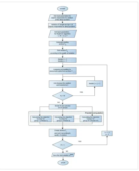
To reconstruct the heat transfer coefficients, it is nec-essary to minimize functionals (15) and (16). For this purpose we use the parallel version of Real Ant Colony Optimization (ACO) algorithm [5, 36]. The ACO algo-rithm was inspired by observation of the ant colonies behavior, widely regarded as the efficient and intelli-gent communities. Because it is a heuristic algorithm, the calculation need to be repeated a certain number of times. In this paper it is ten times. In order to re-duce computation time, we adapted the algorithm for parallel computing. To describe the algorithm, we will use the following notation
F – minimized function, n – dimension (number of variables), nT – number of threads, M = nT · p −
num-ber of ants, I − numnum-ber of iteration, L – numnum-ber of pheromone spots, q, ξ – parameters of the algorithm. Now we present the steps of the algorithm.
Initialization of the algorithm
1 Setting the input parameters of the algorithm L, M, I, nT, q, ξ.
2 Generating randomly L pheromone spots (solu-tions). Assigning them to set T0 (starting archive). 3 Calculating the value of minimized function F for
each pheromone spot and organizing the archive T0 from the best solution to the worst.
Iterative process
4 Assigning probabilities to pheromone spots (solu-tions) according to the following formula
5
By minimization of these functionals we will reconstruct the heat transfer coefficients ℎ, ℎ�, ℎ�.
3 Method of solution
Direct problems, defined by equations (1)-(4) (Model I) and (6)-(11) (Model II), for the fixed values of ℎ, ℎ� and ℎ� is solved by using the implicit finite difference method [3, 7, 23].
To reconstruct the heat transfer coefficients, it is necessary to minimize func-tionals (15) and (16). For this purpose we use the parallel version of Real Ant Colony Optimization (ACO) algorithm [5, 36]. The ACO algorithm was inspired by observa-tion of the ant colonies behavior, widely regarded as the efficient and intelligent com-munities. Because it is a heuristic algorithm, the calculation need to be repeated a cer-tain number of times. In this paper it is ten times. In order to reduce computation time, we adapted the algorithm for parallel computing. To describe the algorithm, we will use the following notation
� − minimized function, � – dimension (number of variables),
�� − number of threads, � = �� � � − number of ants,
� − number of iteration, � – number of pheromone spots,
�, �– parameters of the algorithm. Now we present the steps of the algorithm.
Initialization of the algorithm
1. Setting the input parameters of the algorithm �, �, �, ��, �, �.
2. Generating randomly � pheromone spots (solutions). Assigning them to set �� (starting archive).
3. Calculating the value of minimized function � for each pheromone spot and organizing the archive �� from the best solution to the worst.
Iterative process
4. Assigning probabilities to pheromone spots (solutions) according to the fol-lowing formula
��= ∑�����
��� � = 1,�, � , �,
where wights ωl are associated with l-th solution and expressed by formula
��= 1 ��√��� �
�(���)�
�����.
where wights wl are associated with l-th solution and expressed by formula
5
By minimization of these functionals we will reconstruct the heat transfer coefficients ℎ, ℎ�, ℎ�.
3 Method of solution
Direct problems, defined by equations (1)-(4) (Model I) and (6)-(11) (Model II), for the fixed values of ℎ, ℎ� and ℎ� is solved by using the implicit finite difference method [3, 7, 23].
To reconstruct the heat transfer coefficients, it is necessary to minimize func-tionals (15) and (16). For this purpose we use the parallel version of Real Ant Colony Optimization (ACO) algorithm [5, 36]. The ACO algorithm was inspired by observa-tion of the ant colonies behavior, widely regarded as the efficient and intelligent com-munities. Because it is a heuristic algorithm, the calculation need to be repeated a cer-tain number of times. In this paper it is ten times. In order to reduce computation time, we adapted the algorithm for parallel computing. To describe the algorithm, we will use the following notation
�− minimized function, � – dimension (number of variables),
��− number of threads, � = �� � �− number of ants,
�− number of iteration, � – number of pheromone spots,
�, �– parameters of the algorithm. Now we present the steps of the algorithm.
Initialization of the algorithm
1. Setting the input parameters of the algorithm �, �, �, ��, �, �.
2. Generating randomly � pheromone spots (solutions). Assigning them to set �� (starting archive).
3. Calculating the value of minimized function � for each pheromone spot and organizing the archive �� from the best solution to the worst.
Iterative process
4. Assigning probabilities to pheromone spots (solutions) according to the fol-lowing formula
��= ∑��� � �
��� � = 1,�, � , �,
where wights ωl are associated with l-th solution and expressed by formula
��= 1 ��√��� �
�(���)�
�����.
5 Ant chooses a random l-th solution with probabil-ity pl.
6 Ant transforms the j-th coordinate (j = 1, 2, . . . , n) of l-th solution sjl by proximity sampling with the probability density function (Gaussian function)
5. Ant chooses a random l-th solution with probability pl.
6. Ant transforms the j-th coordinate (j = 1, 2, . . . , n) of l-th solution ��� by
proximity sampling with the probability density function (Gaussian function)
�(�� �� �) = 1 �√��� �
�(���)�
���
where � = ���, � = �
���∑����|���� ���| .
7. Repeating steps 5-6 for each ant. Obtaining M new solutions (pheromone spots).
8. Dividing the new solutions on nT groups. Calculating the value of minimized function F for each new solution (parallel computing).
9. Adding the new solutions to the archive Ti, organizing the archive with respect
to quality, removing M worst solutions. 10. Repeating steps 3 − 9 I times.
where
5. Ant chooses a random l-th solution with probability pl.
6. Ant transforms the j-th coordinate (j = 1, 2, . . . , n) of l-th solution ��� by
proximity sampling with the probability density function (Gaussian function)
�(�� �� �) = 1 �√��� �
�(���)�
���
where � = ���, � = �
���∑����|���� ���| .
7. Repeating steps 5-6 for each ant. Obtaining M new solutions (pheromone spots).
8. Dividing the new solutions on nT groups. Calculating the value of minimized function F for each new solution (parallel computing).
9. Adding the new solutions to the archive Ti, organizing the archive with respect
to quality, removing M worst solutions. 10. Repeating steps 3 − 9 I times.
.
7 Repeating steps 5-6 for each ant. Obtaining M new solutions (pheromone spots).
8 Dividing the new solutions on nT groups. Calculat-ing the value of minimized function F for each new solution (parallel computing).
9 Adding the new solutions to the archive Ti, organiz-ing the archive with respect to quality, removorganiz-ing M worst solutions.
Figure 1
Information Technology and Control 2017/2/46 176
Experimental results
The proposed algorithm was implemented in C# 5.0 on the computer with the following parameters : CPU: Intel Core i5-3230M 2.60GHz; OS: Microsoft Win-dows 10 Home; RAM: 8.00 GB. The multi-threaded calculations were performed by using the Task Paral-lel Library.
Example 1.We consider equation (1) (Model I) with the following data: a = 1.8, t* = 500, x∈[0,1], c = 1000, ρ = 2680, λ = 240, u∞ = 100, f(x) = 100x2, q(t) = 0. The unknown heat transfer coefficient depends on four parameters (which have to be reconstructed) in the following form
4 Experimental results
The proposed algorithm was implemented in C# 5.0 on the computer with the following parameters : CPU: Intel Core i5-3230M 2.60GHz; OS: Microsoft Windows 10 Home; RAM: 8.00 GB. The multi-threaded calculations were performed by using the Task Parallel Library.
Example 1. We consider equation (1) (Model I) with the following data: � = 1.8, �∗=
500, � ∈ [0,1], � = 1000, � = 2�80, � = �2�0, ��= 100, �(�) = 100��,
�(�) = 0. The unknown heat transfer coefficient depends on four parameters (which
have to be reconstructed) in the following form
ℎ(�) = � �
����, � ∈ [0,100]. �, � ∈ (100,200], ��, � ∈ (200,350], ��, � ∈ (350,500].
The exact values of sought parameters ��, ��, �� and �� are equal to 2000, 1400, 800
and 250, respectively.
As a result of solving the direct problem for the exact heat transfer coefficient h, we obtain the values of temperature at the selected points in the grid of domain D. Then, from these values we select only those ones corresponding to the predetermined grid points (location of the thermocouple). These values simulate the temperature meas-urements. We call them the exact input data and denote by ����. The grid used to
gener-ate these data was of size 200 × 1000.
There is one measurement point xp = 0.18 (N1 = 1), the measurements from
this point will be read every 1s and 2s (N2 = 501, 251). In order to investigate the impact
of measurement errors on the results of reconstruction and stability of the algorithm, the input data were perturbed by the pseudo-random error of sizes 1 and 2%.
In the process of reconstructing the boundary condition (minimizing the func-tional), the direct problem was solved many times. The grid used for this purpose was of size 150 × 500 and had different density than the grid used to generate the input data. Minimum of functional (15) was searched by using the ACO algorithm. This
algorithm is heuristic, therefore it is required to repeat calculations a certain number of times. In this paper, we assumed that the calculations for each case were repeated ten times. Algorithm was adapted for parallel computations (multi-threaded calculations) which significantly reduced the computational time. In ACO algorithm, we set the fol-lowing parameters
�� = �,���� = 12,���� = 8,���� = 30, ��∈ [1800, 2300], ��∈ [1200, 1700],
��∈ [500, 1000], ��∈ [100, 500].
Thus, the number of minimized function calls was equal to 368.
Table 1 presents the results of determining a1, a2, a3, a4 in dependence on the size of
input data disturbance at the measurement point xp = 0.18 for measurements taken at The exact values of sought parameters a1, a2, a3 and a4 are equal to 2000, 1400, 800 and 250, respectively. As a result of solving the direct problem for the exact heat transfer coefficient h, we obtain the values of temperature at the selected points in the grid of do-main D. Then, from these values we select only those ones corresponding to the predetermined grid points (location of the thermocouple). These values simu-late the temperature measurements. We call them the exact input data and denote by
�(�, �, �) = �(�, �), � � [�, ��], � � ��, ���, (7)
���(�, �, �) ��(�,�,�)�� = ��(�, �), � � [�, �∗], � � [�, ��],
(8)
�����, ��, �� ����,����,��= ��(�, �), � � [�, �∗], � � [�, ��], (9)
���(�, �, �)��(�,�,�)�� = ℎ�(�, �)(�(�, �, �) � ��), � � [�, �∗], � � ��, ���, (10)
���(��, �, �)��(����,�,�)= ℎ�(�, �)(�(��, �, �) � ��), � � [�, �∗], � � ��, ���, (11)
���(�,�) ��� = � �(���)� ���(�,�) ��� (� � �)����� ��, �
� (12)
where Γ is the Gamma function and � � (� � �, �].
�(��, ��) = ����, � = �,�, � , ��, � = �,�, � , ��, (Model I) (13)
����, ��, ��� = ��(��)�, (��) = �,�, � , ��, � = �,�, � , ��, (Model II) (14)
�(ℎ) = ∑ ∑����� ����� ����(ℎ) � ������,
(for Model I), (15)
�(ℎ�, ℎ�) = ∑�(��)��� ∑����� ��(��)�(ℎ�, ℎ�) � ��(��)���,
(for Model II). (16)
. The grid used to generate these data was of size 200 × 1000.
There is one measurement point xp = 0.18 (N1 = 1), the measurements from this point will be read every 1s and 2s (N2 = 501, 251). In order to investigate the impact of measurement errors on the results of reconstruction and stability of the algorithm, the input data were per-turbed by the pseudo-random error of sizes 1 and 2%. In the process of reconstructing the boundary condi-tion (minimizing the funccondi-tional), the direct problem was solved many times. The grid used for this purpose was of size 150 × 500 and had different density than the grid used to generate the input data.
Minimum of functional (15) was searched by using the ACO algorithm. This algorithm is heuristic, there-fore it is required to repeat calculations a certain number of times. In this paper, we assumed that the calculations for each case were repeated ten times.
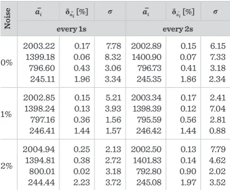
Table 1
Results of calculations in case of measurements ae every 1s, 2s (ai– – restored value of ai, δai– percentage relative error of ai, σ - standard deviation (i = 1, 2, 3, 4))
N
oise ai
– δ
ai– [%] σ a–i δai– [%] σ
every 1s every 2s
0% 2003.22 1399.18 796.60 245.11 0.17 0.06 0.43 1.96 7.78 8.32 3.06 3.34 2002.89 1400.90 796.73 245.35 0.15 0.07 0.41 1.86 6.15 7.33 3.18 2.34 1% 2002.85 1398.24 797.16 246.41 0.15 0.13 0.36 1.44 5.21 3.93 1.56 1.57 2003.34 1398.39 795.59 246.42 0.17 0.12 0.56 1.44 2.41 7.04 2.81 0.88 2% 2004.94 1394.81 800.01 244.44 0.25 0.38 0.02 2.23 2.13 2.72 3.18 3.72 2002.50 1401.83 792.80 245.08 0.13 0.14 0.90 1.97 7.79 4.62 2.02 3.52
Algorithm was adapted for parallel computations (multi-threaded calculations) which significantly re-duced the computational time. In ACO algorithm, we set the following parameters
nT = 4, M = 12, L = 8, I = 30, a1∈[1800, 2300], a2∈ [1200, 1700], a3∈[500, 1000], a4∈[100, 500].
Thus, the number of minimized function calls was equal to 368.
Table 1 presents the results of determining a1, a2, a3, a4 in dependence on the size of input data disturbance
at the measurement point xp = 0.18 for measurements taken at every 1s and 2s. Generally, the obtained re-sults are quite good. Except the error of parameter a4 restoration, the other errors do not exceed the input data errors. Maximal error of parameter a4 recon-struction is equal to 2.23%, in case of the other param-eters the errors do not exceed 0.91%.
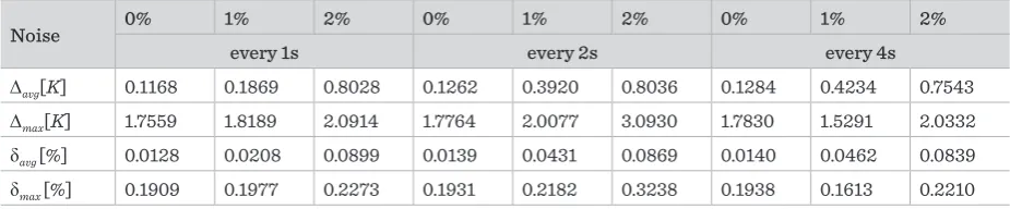
Table 2
Errors of temperature reconstruction in measurement point xp = 0.18 for measurements at every 1, 2s (∆avg
–
average absolute error, ∆max – maximal absolute error, δavg –
average relative error, δmax – maximal relative error)
N
oise
0% 1% 2% 0% 1% 2%
every 1s every 2s
∆avg[K] 0.0070 0.0113 0.0175 0.0097 0.0116 0.0278
∆max[K] 0.0846 0.0846 0.0850 0.0846 0.0847 0.0845
δavg [%] 0.0424 0.0546 0.0663 0.0487 0.0524 0.0977
δmax [%] 2.3406 2.3384 2.3508 2.3386 2.3413 2.3363
Figure 1 shows the relative errors of reconstructing the heat transfer coefficient h for measurements at every 1, 2s. This error was calculated according to the formula
��=∥ ℎ�(�) � ℎ(�) ∥∥ ℎ(�) ∥ ∙ 100 [%],
where ℎ�(�), ℎ(�) describe the reconstructed and exact heat transfer coefficient, respec-tively, and ∥ ∙ ∥ denotes the norm defined by the following formula
‖�(�)‖ = �� |�(�)|� �
∗
� �
� �
.
These errors are minimal and smaller than 0.42%. For measurements every one second, relative error of reconstruction heat conduction coefficient for exact input data is sligh-tly greater than in case of 1% perturbed input data. The reason for this it could be pro-babilistic character of Real Ant Colony Optimization algorithm.
Fig. 2. Relative errors of reconstructing the heat transfer coefficient for various perturbations of input data and for measurements at every 1s and 2s
Figure 2 presents the distribution of errors of the temperature reconstruction in meas-urement point xp = 0.18 in case of measurements at every 2s.
where ĥ(t), h(t) describe the reconstructed and exact
heat transfer coefficient, respectively, and ��=∥ ℎ�(�) � ℎ(�) ∥∥ ℎ(�) ∥ ∙ 100 [%],
where ℎ�(�), ℎ(�) describe the reconstructed and exact heat transfer coefficient, respec-tively, and ∥ ∙ ∥ denotes the norm defined by the following formula
‖�(�)‖ = �� |�(�)|� �
∗
� �
� �
.
These errors are minimal and smaller than 0.42%. For measurements every one second, relative error of reconstruction heat conduction coefficient for exact input data is sligh-tly greater than in case of 1% perturbed input data. The reason for this it could be pro-babilistic character of Real Ant Colony Optimization algorithm.
Fig. 2. Relative errors of reconstructing the heat transfer coefficient for various perturbations of input data and for measurements at every 1s and 2s
Figure 2 presents the distribution of errors of the temperature reconstruction in meas-urement point xp = 0.18 in case of measurements at every 2s.
∙
��=∥ ℎ�(�) � ℎ(�) ∥∥ ℎ(�) ∥ ∙ 100 [%],
where ℎ�(�), ℎ(�) describe the reconstructed and exact heat transfer coefficient, respec-tively, and ∥ ∙ ∥ denotes the norm defined by the following formula
‖�(�)‖ = �� |�(�)|� �
∗
� �
� �
.
These errors are minimal and smaller than 0.42%. For measurements every one second, relative error of reconstruction heat conduction coefficient for exact input data is sligh-tly greater than in case of 1% perturbed input data. The reason for this it could be pro-babilistic character of Real Ant Colony Optimization algorithm.
Fig. 2. Relative errors of reconstructing the heat transfer coefficient for various perturbations of input data and for measurements at every 1s and 2s
Figure 2 presents the distribution of errors of the temperature reconstruction in meas-urement point xp = 0.18 in case of measurements at every 2s.
de-notes the norm defined by the following formula
��=∥ ℎ�(�) � ℎ(�) ∥∥ ℎ(�) ∥ ∙ 100 [%],
where ℎ�(�), ℎ(�) describe the reconstructed and exact heat transfer coefficient,
respec-tively, and ∥ ∙ ∥ denotes the norm defined by the following formula
‖�(�)‖ = �� |�(�)|� �
∗
� �
� �
.
These errors are minimal and smaller than 0.42%. For measurements every one second, relative error of reconstruction heat conduction coefficient for exact input data is sligh-tly greater than in case of 1% perturbed input data. The reason for this it could be pro-babilistic character of Real Ant Colony Optimization algorithm.
Fig. 2. Relative errors of reconstructing the heat transfer coefficient for various perturbations of input data and for measurements at every 1s and 2s
Figure 2 presents the distribution of errors of the temperature reconstruction in
meas-urement point xp = 0.18 in case of measurements at every 2s.
These errors are minimal and smaller than 0.42%. For measurements every one second, relative error of reconstruction heat conduction coefficient for exact input data is slightly greater than in case of 1% per-turbed input data. The reason for this it could be pro-babilistic character of Real Ant Colony Optimization algorithm.
Figure 2 presents the distribution of errors of the temperature reconstruction in measurement point xp = 0.18 in case of measurements at every 2s.
We can see that the error of temperature reconstruc-tion depends on perturbareconstruc-tions of the input data. The input errors are larger, the errors of temperature re-constuction increase. Generally, the temperature is reconstructed very well.
Figure 2
Relative errors of reconstructing the heat transfer coefficient for various perturbations of input data and for measurements at every 1s and 2s
Figure 3
Distribution of errors of temperature reconstruction in measurement point xp = 0.18 for measurements at every 2s
and for various perturbations of input data (0% – dotted line, 1% – dashed line, 2% – solid line)
Example 2.In this example, we consider equation (6) (Model II) with the following data:
t* = 100, x∈[0, 0.2], y∈[0, 0.2],
c = 1000, ρ = 2680, a = 0.4, λ1(x, y, t) = λ2(x, y, t) = 240, u∞ = 300, f(x, y) = 900, q1(t, x) = q2(t, x) = 0, g(x, y, t) = 0.
Information Technology and Control 2017/2/46 178
11
Fig. 3. Distribution of errors of temperature reconstruction in measurement point xp = 0.18 for
measurements at every 2s and for various perturbations of input data (0% – dotted line, 1% – dashed line, 2% – solid line)
We can see that the error of temperature reconstruction depends on perturbations of the input data. The input errors are larger, the errors of temperature reconstuction in-crease. Generally, the temperature is reconstructed very well.
Example 2. In this example, we consider equation (6) (Model II) with the following
data: �∗= 100, � � [0, 0.2], � � [0, 0.2], � = 1000, � = 26�0, � =
0.4, ��(�, �, �) = ��(�, �, �) = 240, ��= 300, �(�, �) = 900, ��(�, �) =
��(�, �) = 0, �(�, �, �) = 0.
Each of the unknown heat transfer coefficients depends on three parameters in the fol-lowing form
ℎ�(�, �) = �
��, � � [0, 30],
��, � � (30, 70],
��, � � (70, 100],
ℎ�(�, �) = �
��, � � [0, 30],
��, � � (30, 70],
��, � � (70, 100].
To restore the Robin boundary conditions, we need to find parameters ��, ��, � , ��. In this numerical experiment the exact values of parameters �� (� = 1,2, � ,6) are equal to 1200, 800, 300, 900, 600, 150, respectively. In order to generate the input data, we used the grid of size 200 × 200 × 200, but in process of solving the inverse problem we used the grid of size 100 × 100 × 100. We obtained thus the measurements for four measurement points (��= 4) with the following spatial coordinates : �(0.004, 0.19),
�(0.004, 0.17), �(0.196, 0.01), �(0.196, 0.03). Distribution of the measurement
points is presented in Figure 3.
.
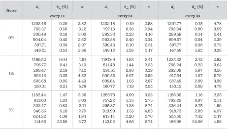
To restore the Robin boundary conditions, we need to find parameters b1, b2, ..., b6. In this numerical experi-ment the exact values of parameters bi(i = 1, 2, ..., 6) are equal to 1200, 800, 300, 900, 600, 150, respectively. In order to generate the input data, we used the grid of size 200 × 200 × 200, but in process of solving the in-verse problem we used the grid of size 100 × 100 × 100. We obtained thus the measurements for four mea-surement points (N1 = 4) with the following spatial coordinates : A(0.004, 0.19), B(0.004, 0.17), C(0.196, 0.01), D(0.196, 0.03). Distribution of the measurement points is presented in Figure 4.
The parameters of the algorithm are as follows: M = 16, L = 8, I = 30, nT= 8,
Table 3
Results of calculation in case of measurements at every 1s, 2s (bi – restored value of b–i, δbi– – percentage relative error of bi,
σ – standard deviation (i = 1, 2, 3, 4, 5, 6))
Noise a–i δai– [%] σ a–i δai– [%] σ a–i δai– [%] σ
every 1s every 2s every 4s
0% 1203.46 795.37 300.48 904.04 597.71 149.21 0.29 0.58 0.16 0.45 0.38 0.53 2.82 3.12 3.03 2.62 2.97 2.66 1202.18 797.13 293.33 903.58 599.43 148.12 0.19 0.36 2.23 0.40 0.10 1.26 2.58 2.94 4.16 3.04 2.61 3.17 1201.77 792.84 299.59 899.67 597.77 147.58 0.15 0.90 0.14 0.04 0.38 1.62 4.78 3.59 3.41 2.39 3.73 3.38 1% 1199.52 796.77 293.47 903.13 605.68 150.31 0.04 0.41 2.18 0.35 0.95 0.21 4.51 3.10 7.12 4.82 4.43 5.78 1187.69 811.48 291.51 900.55 609.84 160.77 1.03 1.44 2.83 0.07 1.65 7.19 3.41 2.03 3.29 3.59 2.87 2.55 1225.32 798.24 282.09 917.64 587.49 153.12 2.12 0.22 5.97 1.97 2.09 2.09 2.62 3.63 3.56 5.79 3.39 4.79 2% 1182.44 813.03 302.47 946.56 624.32 114.66 1.47 1.63 0.82 5.18 4.06 23.56 3.26 3.03 3.11 2.79 1.94 2.72 1259.78 757.22 295.87 913.90 613.14 143.02 4.99 5.35 1.38 1.55 2.20 4.66 3.03 2.75 8.74 4.83 5.76 5.74 1186.09 792.29 326.24 918.73 555.50 186.08 1.16 0.97 8.75 2.09 7.42 24.06 2.35 2.31 4.99 4.07 5.17 4.56 Figure 4
Distribution of the measurement points
b1∈[1000, 1400], b2∈[600, 1000], b3∈[100, 500], b4∈[700, 1100], b5∈[400, 800], b6∈[50, 350].