R E S E A R C H
Open Access
The new modified Ishikawa iteration method
for the approximate solution of different
types of differential equations
Necdet Bildik, Yasemin Bakır and Ali Mutlu
**Correspondence:
[email protected] Department of Mathematics, Faculty of Science and Arts, Celal Bayar University, Muradiye Campus, Manisa, 45047, Turkey
Abstract
In this article, the new Ishikawa iteration method is presented to find the approximate
solution of an ordinary differential equation with an initial condition. Additionally,
some numerical examples with initial conditions are given to show the properties of
the iteration method. Furthermore, the results of absolute errors are compared with
Euler, Runge-Kutta and Picard iteration methods. Finally, the present method, namely
the new modified Ishikawa iteration method, is seen to be very effective and efficient
in solving different type of the problem.
MSC:
65K15; 65L07; 65L06; 65L70
Keywords:
ordinary differential equation; Euler method; fixed point; numerical
analysis; modified Ishikawa iteration; Picard successive iteration method
Introduction
Various kinds of numerical methods, especially iterative methods [–], were used to solve
different types of differential equations. In recent years, there has been a growing interest
in the treatment of iterative approximation of fixed point theory on normed linear spaces
[–], Banach spaces [–] and Hilbert spaces [, ], respectively.
A new modified Ishikawa iteration method has been developed to find an approximate
solution for different types of differential equations with initial conditions [, –] on
metric spaces. The solutions are also obtained in terms of the Picard iteration. Also in
Section , examples of these kinds of equations are solved using this new method which
is called new modified Ishikawa iteration method and also the results are discussed and
comparison using Euler [, ], Runge-Kutta [, ], and Picard iteration methods [, ,
] is presented in tables and figures. Additionally, this approximated method can solve
various different differential equations such as integral, difference, integro-differential and
functional differential equations. Finally, numerical results shows that the new modified
Ishikawa iteration method is more or less effective and also convenient for solving different
types of differential equations.
Now, let us give some of the important theorems and definitions in order to solve linear
and nonlinear differential equations using a contraction mapping.
1 Preliminaries
Theorem .
(Banach contraction principle)
Let
(X,
d)
be a complete metric space and
T
:
X
→
X be a contraction with the Lipschitzian constant L.
Then T has a unique fixed
point u
∈
X.
Furthermore,
for any x
∈
X we have
lim
n→∞
T
n
(x) =
u
with
d
T
n(x),
u
≤
L
n
–
L
d
x,
F(x)
(see
[]).
Proof
We first show uniqueness. Suppose there exist
x,
y
∈
X
with
T
(x) =
x
and
T
(y) =
y.
Then
d(x,
y) =
d
T
(x),
T(y)
≤
Ld(x,
y),
therefore
d(x,
y) = .
To show existence select,
x
∈
X. We first show that
{T
n(x)}
is a Cauchy sequence. Notice
for
n
∈ {, , . . .}
that
d
T
n(x),
T
n+(x)
≤
Ld
T
n–(x),
T
nx
≤ · · · ≤
L
nd
x,
T
(x)
.
Thus, for
m
>
n
where
n
∈ {
, , . . .
}
,
d
T
n(x),
T
m(x)
≤
d
T
n(x),
T
n+(x)
+
d
T
n+(x),
T
n+(x)
+
· · ·
+
≤ · · · ≤
d
T
m–(x),
T
m(x)
≤
L
nd
x,
T
(x)
+
· · ·
+
L
m–d
x,
T(x)
≤
L
nd
x,
T
(x)
+
L
+
L
+
· · ·
=
L
n
–
L
d
x,
T(x)
.
That is, for
m
>
n,
n
∈ {
, , . . .
}
,
d
T
n(x),
T
m(x)
≤
L
n
–
L
d
x,
T
(x)
.
(.)
This shows that
{T
n(x)}
is a Cauchy sequence and since
X
is complete, there exists
u
∈
X
with
lim
n→∞T
n(x) =
u. Moreover, the continuity of
T
yields
u
=
lim
n→∞
T
n+
(x) =
lim
n→∞
T
T
n(x)
=
T(u),
therefore
u
is a fixed point of
T
. Finally, letting
m
→ ∞
in (.) yields
d
T
n(x),
u
≤
L
n
–
L
d
Corollary .
Let
(X,
d)
be a complete metric space and let B(x
,
r) =
{x
∈
X
:
d(x,
x
) <
r},
where x
∈
X and r
> .
Suppose T
:
B(x
,
r)
→
X is a contraction
(that is,
d(T
(x),
T
(y))
≤
Ld(x,
y)
for all x,
y
∈
B(x
,
r)
with
≤
L
< )
with d(T
(x
),
x
) < (–L)r.
Then T has a unique
fixed point in B(x
,
r) (see
[]).
Definition .
If the sequence
{x
n}
∞n=provides the condition
x
n+=
Tx
nfor
n
= , , , . . . ,
then this is called the Picard iteration [, ].
Definition .
Let
x
∈
X
be arbitrary. If the
{x
n}
∞n=sequence provides the condition
x
n+= ( –
α
n)x
n+
{
α
n}
Ty
n,
y
n= ( –
β
n)x
n+
{
β
n}
Tx
nfor
n
= , , , . . . , then this is called the Ishikawa iteration [, ] where (
α
n) and (
β
n) are
sequences of positive numbers that satisfy the following conditions:
(i)
≤
α
n≤
β
n< , for all positive integers
n,
(ii)
lim
n→∞β
n= ,
(iii)
n≥α
nβ
n=
∞
.
Definition .
If
λ
∈
[, ],
γ
∈
[, ] and
y
∈
X,
T
is defined as a contraction mapping
with regard to Picard iteration and also the
{
y
n}
∞n=sequence provides the conditions
y
n+=
λ
y
n–+ ( –
λ
)Ty
n–,
y
n= ( –
γ
)y
n–+
γ
Ty
n–,
n
= , , . . . ,
y
n+=
y
+
xx
F
t,
y
n(t)
dt,
n
= ,
Ty
n–=
y
n,
<
λ
,
μ
<
then this is called a new modified Ishikawa iteration where
T
=
xx
F(t,
y
n(t))
dt.
In order to illustrate the performance of the new modified Ishikawa iteration method in
solving linear and nonlinear differential equations and justify the accuracy and efficiency
of the method presented in this paper, we consider the following examples. In all examples,
we used four types of iteration methods and the comparison is shown in figures and tables
respectively.
2 Application of methods
Example .
Let us consider the differential equation
y
=
|y|
subject to the initial
con-dition
y() = .
Firstly, we obtained the exact solution of the equation as
|y|
=
(x
+ )
= +
x
+
x
.
By Theorem . and Corollary ., since
T
=
xx
F(t,
y
n(t))dt, then
T
(x) –
T
(y)
=
x
√
t dt
–
y
√
t dt
=
√
t
x
–
√
t
y
≤
√
x
–
y
≤
So,
|T(x) –
T
(y)| ≤
|x
–
y|
is found. Thus
T
has a unique fixed point, which is the unique
solution of the integral equation
T
=
xx
F(t,
y
n(t))dt
or the differential equation
y
=
|y|,
y() = .
Firstly, we approach the approximate solution using by the Picard iteration method.
Thus
y
= +
x,
y
=
+
(x
+ )
/
are obtained. If we take the series expansion of the function (x
+ )
/for the seven terms,
then
y
= +
x
+
x +
x
+
x
+
x
+
x
is found. Now, applying the new modified Ishikawa
iteration method to the equation for
λ
= .,
γ
= .,
y
= +
x,
y
= + .x,
y
= + .x,
y
= + .x,
y
= + .x,
y
= + .x,
y
= + .x,
y
= + .x,
y
= + .x,
y
= + .x,
y
= + .x
are found and also for
λ
= .,
γ
= .,
y
= +
x,
y
= + .x,
y
= + .x,
y
= + .x,
y
= + .x,
y
= + .x,
y
= + .x,
y
= + .x,
y
= + .x,
y
= + .x,
are obtained. On the other hand, for
λ
= .,
γ
= .,
y
= +
x,
y
= + .x,
y
= + .x,
y
= + .x,
y
= + .x,
y
= + .x,
y
= + .x,
y
= + .x,
y
= + .x,
y
= + .x,
y
= + .x
are calculated. In the same way, for
λ
= .,
γ
= .,
y
= +
x,
y
= + .x,
y
= + .x,
y
= + .x,
y
= + .x,
y
= + .x,
y
= + .x,
y
= + .x,
y
= + .x,
y
= + .x,
y
= + .x
are found and also for
λ
= .,
γ
= .,
y
= +
x,
y
= + .x,
y
= + .x,
y
= + .x,
y
= + .x,
y
= + .x,
y
= + .x,
y
= + .x,
y
= + .x,
y
= + .x
are obtained. Similarly, for
λ
= .,
γ
= .,
y
= +
x,
y
= + .x,
y
= + .x,
y
= + .x,
y
= + .x,
y
= + .x,
y
= + .x,
y
= + .x,
y
= + .x,
y
= + .x,
y
= + .x
are calculated. Finally, for
λ
= .,
γ
= .,
y
= +
x,
y
= + .x,
y
= + .x,
y
= + .x,
y
= + .x,
y
= + .x,
y
= + .x,
y
= + .x,
y
= + .x,
y
= + .x,
y
= + .x
Now we calculate the approximate solution by the Euler method. At first we use the
formula
y
n+=
y
n+
hF(x
n,
y
n)
with
F(x,
y) =
|
y
|,
h
= . and
x
= ,
y
= . From the initial condition
y() = , we have
F(, ) = . We now proceed with the calculations as follows:
F
=
F(, ) = ,
y
=
y
+
hF
= + .,
y
= .,
F
=
F(., .) = .,
y
= . + .F
,
y
= .,
F
=
F(., .) = .,
y
= . + .F
,
y
= ..
Finally, applying the Runge-Kutta method to the given initial value problem, we carry out
the intermediate calculations in each step to give figures after the decimal point and round
off the final results at each step to four such places. Here
F(x,
y) =
|y|x
= ,
y
= and
we are to use
h
= .. Using these quantities, we calculated successively
k
,
k
,
k
,
k
and
K
defined by
k
=
hg(y
,
x
),
k
=
hg
y
+
h
,
x
+
k
,
k
=
hg
y
+
h
,
x
+
k
,
k
=
hg(y
+
h,
x
+
k
)
and
K
=
(k
+ k
+ k
+
k
),
y
n+=
y
n+
K
. Thus we find
k
,
k
,
k
,
k
for
n
= as
follows:
k
= .F(x
,
y
) = .F(, ) = .,
k
= .F(x
+ .,
y
+ .) = .,
k
= .F(x
+ .,
y
+ .) = .,
So,
y
= . is obtained for
x
= .. On the other hand, we calculated
k
,
k
,
k
,
k
for
n
= as follows:
k
= .F(x
,
y
) = .F(., .) = .,
k
= .F(x
+ .,
y
+ .) = .,
k
= .F(x
+ .,
y
+ .) = .,
k
= .F(x
+ .,
y
+ .) = ..
Hence
y
= . is calculated for
x
= .. Finally we get
k
,
k
,
k
,
k
for
n
= as
follows:
k
=
hF(x
,
y
) = .,
k
=
hF
x
+
h
,
y
+
k
= .,
k
=
hF
x
+
h
,
y
+
k
= .,
k
=
hF(x
+
h,
y
+
k
) = ..
Thus,
y
= . is obtained for
x
= ..
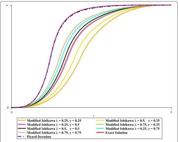
After the necessary calculation which is done above, the comparison is shown
schemat-ically in Figure .
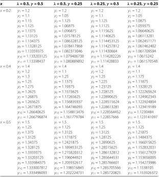
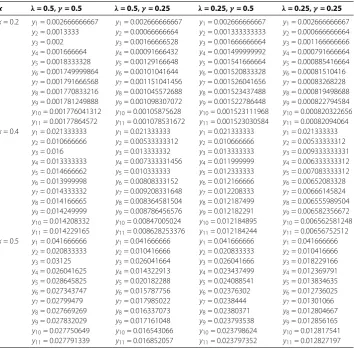
Table 1 The solutions obtained by the new modified Ishikawa iteration method for different
values of
λ
and
γ
x λ= 0.5,γ= 0.5 λ= 0.5,γ= 0.25 λ= 0.25,γ= 0.5 λ= 0.25,γ= 0.25 x= 0.2 y1= 1.2
y2= 1.1
y3= 1.15
y4= 1.125
y5= 1.1375
y6= 1.13125
y7= 1.134375
y8= 1.1328125
y9= 1.13359375
y10= 1.133203125
y11= 1.13398437
y1= 1.2
y2= 1.05
y3= 1.125
y4= 1.06875
y5= 1.096875
y6= 1.07578125
y7= 1.086328125
y8= 1.078417968
y9= 1.082373046
y10= 1.079406738
y11= 1.080889892
y1= 1.2
y2= 1.1
y3= 1.125
y4= 1.1125
y5= 1.115625
y6= 1.1140625
y7= 1.114453125
y8= 1.114257812
y9= 1.11430664
y10= 1.114282226
y11= 1.11428833
y1= 1.2
y2= 1.05
y3= 1.0875
y4= 1.059375
y5= 1.06640625
y6= 1.06113281
y7= 1.062451171
y8= 1.061462402
y9= 1.061709594
y10= 1.0615242
y11= 1.061570548
x= 0.4 y1= 1.4
y2= 1.2
y3= 1.3
y4= 1.25
y5= 1.275
y6= 1.2625
y7= 1.26875
y8= 1.265625
y9= 1.2671875
y10= 1.26640625
y11= 1.266796874
y1= 1.4
y2= 1.1
y3= 1.25
y4= 1.1375
y5= 1.19375
y6= 1.1515625
y7= 1.17265625
y8= 1.156835937
y9= 1.164746093
y10= 1.158813476
y11= 1.161779784
y1= 1.4
y2= 1.2
y3= 1.25
y4= 1.225
y5= 1.23125
y6= 1.228125
y7= 1.22890625
y8= 1.228515624
y9= 1.228613281
y10= 1.228564452
y11= 1.22857666
y1= 1.4
y2= 1.1
y3= 1.175
y4= 1.11875
y5= 1.1328125
y6= 1.122265624
y7= 1.124902343
y8= 1.122924804
y9= 1.123419189
y10= 1.1230484
y11= 1.123141097
x= 0.5 y1= 1.5
y2= 1.25
y3= 1.375
y4= 1.3125
y5= 1.34375
y6= 1.328125
y7= 1.3359375
y8= 1.33203125
y9= 1.333984375
y10= 1.333007812
y11= 1.333496093
y1= 1.5
y2= 1.125
y3= 1.3125
y4= 1.171875
y5= 1.2421875
y6= 1.189453125
y7= 1.215820312
y8= 1.196044921
y9= 1.205932617
y10= 1.198516845
y11= 1.202224731
y1= 1.5
y2= 1.25
y3= 1.3125
y4= 1.28125
y5= 1.2890625
y6= 1.28515625
y7= 1.286132812
y8= 1.285644531
y9= 1.285766601
y10= 1.285705566
y11= 1.285720825
y1= 1.5
y2= 1.125
y3= 1.21875
y4= 1.1484375
y5= 1.166015625
y6= 1.152832031
y7= 1.156127929
y8= 1.153656005
y9= 1.154273986
y10= 1.1538105
y11= 1.153926372
On the other hand, we may give Table , Table , Table and Table using the modified
Ishikawa iteration method for different values of
λ
and
γ
. Now we may give Table which
is expressed that absolute error of Example . for different values of
λ
and
γ
with
x
= .,
x
= . and
x
= . respectively.
Corollary .
If we compare the approximate solution with the different values of
λ
and
γ
,
then the conclusion may be indicated using Table
,
Table
,
Table
and Table
as follows.
The best approximation is obtained taking the different values of
λ
and
γ
and using the
new modified Ishikawa iteration method for x
= .,
x
= .
and x
= .
getting
(
λ
= .,
γ
= .;
λ
= .,
γ
= .;
λ
= .,
γ
= .;
λ
= .,
γ
= .;
λ
= .,
γ
= .;
λ
= .,
γ
= .;
λ
= .,
γ
= .)
respectively.
Similarly,
we calculated the solution for x
= .,
x
=
and x
= .
then the approximation
is found more sensitive taking
(
λ
= .,
γ
= .;
λ
= .,
γ
= .;
λ
= .,
γ
= .;
λ
= .,
γ
= .;
λ
= .,
γ
= .;
λ
= .,
γ
= .;
λ
= .,
γ
= .)
respectively.
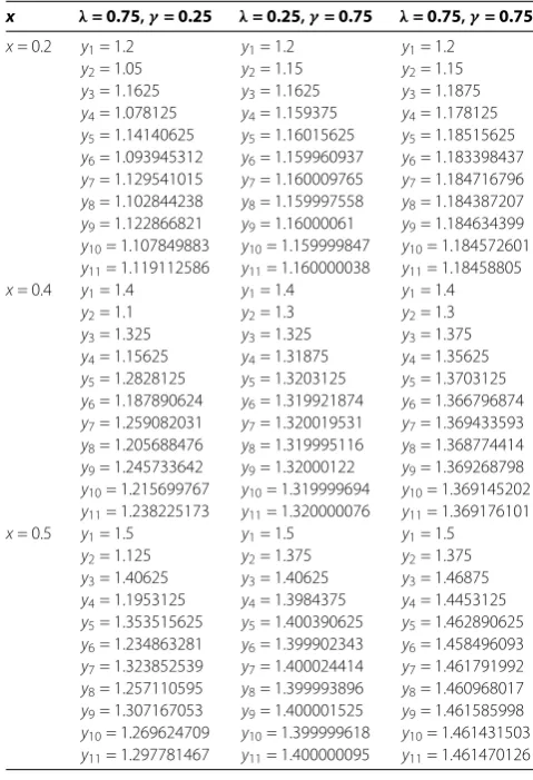
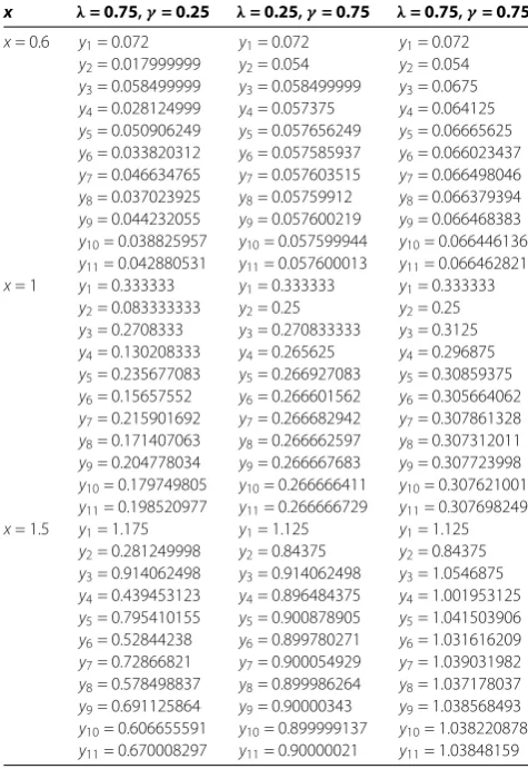
Table 2 The solutions obtained by the new modified Ishikawa iteration method for different
values of
λ
and
γ
x λ= 0.75,γ= 0.25 λ= 0.25,γ= 0.75 λ= 0.75,γ= 0.75 x= 0.2 y1= 1.2
y2= 1.05
y3= 1.1625
y4= 1.078125
y5= 1.14140625
y6= 1.093945312
y7= 1.129541015
y8= 1.102844238
y9= 1.122866821
y10= 1.107849883
y11= 1.119112586
y1= 1.2
y2= 1.15
y3= 1.1625
y4= 1.159375
y5= 1.16015625
y6= 1.159960937
y7= 1.160009765
y8= 1.159997558
y9= 1.16000061
y10= 1.159999847
y11= 1.160000038
y1= 1.2
y2= 1.15
y3= 1.1875
y4= 1.178125
y5= 1.18515625
y6= 1.183398437
y7= 1.184716796
y8= 1.184387207
y9= 1.184634399
y10= 1.184572601
y11= 1.18458805
x= 0.4 y1= 1.4
y2= 1.1
y3= 1.325
y4= 1.15625
y5= 1.2828125
y6= 1.187890624
y7= 1.259082031
y8= 1.205688476
y9= 1.245733642
y10= 1.215699767
y11= 1.238225173
y1= 1.4
y2= 1.3
y3= 1.325
y4= 1.31875
y5= 1.3203125
y6= 1.319921874
y7= 1.320019531
y8= 1.319995116
y9= 1.32000122
y10= 1.319999694
y11= 1.320000076
y1= 1.4
y2= 1.3
y3= 1.375
y4= 1.35625
y5= 1.3703125
y6= 1.366796874
y7= 1.369433593
y8= 1.368774414
y9= 1.369268798
y10= 1.369145202
y11= 1.369176101
x= 0.5 y1= 1.5
y2= 1.125
y3= 1.40625
y4= 1.1953125
y5= 1.353515625
y6= 1.234863281
y7= 1.323852539
y8= 1.257110595
y9= 1.307167053
y10= 1.269624709
y11= 1.297781467
y1= 1.5
y2= 1.375
y3= 1.40625
y4= 1.3984375
y5= 1.400390625
y6= 1.399902343
y7= 1.400024414
y8= 1.399993896
y9= 1.400001525
y10= 1.399999618
y11= 1.400000095
y1= 1.5
y2= 1.375
y3= 1.46875
y4= 1.4453125
y5= 1.462890625
y6= 1.458496093
y7= 1.461791992
y8= 1.460968017
y9= 1.461585998
y10= 1.461431503
y11= 1.461470126
Example .
Let us consider the differential equation
y
=
y
+
x
subject to the initial condition
y() = .
Firstly, we obtained the exact solution of the equation as
y
= e
x–
x
– x
– .
Using Theorem . and Corollary ., since
T
=
xx
F(t,
y
n(t))dt, then
T
has a unique
fixed point, which is the unique solution of the differential equation
y
=
y
+
x
with the
initial condition
y() = .
At first, we approach the approximate solution by the Picard iteration method as follows:
y
=
x
,
y
=
x
+
x
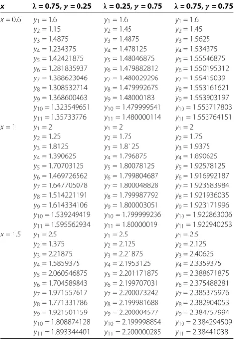
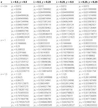
Table 3 The solutions obtained by the new modified Ishikawa iteration method for different
values of
λ
and
γ
x λ= 0.75,γ= 0.25 λ= 0.25,γ= 0.75 λ= 0.75,γ= 0.75 x= 0.6 y1= 1.6
y2= 1.15
y3= 1.4875
y4= 1.234375
y5= 1.42421875
y6= 1.281835937
y7= 1.388623046
y8= 1.308532714
y9= 1.368600463
y10= 1.323549651
y11= 1.35733776
y1= 1.6
y2= 1.45
y3= 1.4875
y4= 1.478125
y5= 1.48046875
y6= 1.479882812
y7= 1.480029296
y8= 1.479992675
y9= 1.48000183
y10= 1.479999541
y11= 1.480000114
y1= 1.6
y2= 1.45
y3= 1.5625
y4= 1.534375
y5= 1.55546875
y6= 1.550195312
y7= 1.55415039
y8= 1.553161621
y9= 1.553903197
y10= 1.553717803
y11= 1.553764151
x= 1 y1= 2
y2= 1.25
y3= 1.8125
y4= 1.390625
y5= 1.70703125
y6= 1.469726562
y7= 1.647705078
y8= 1.514221191
y9= 1.614334106
y10= 1.539249419
y11= 1.595562934
y1= 2
y2= 1.75
y3= 1.8125
y4= 1.796875
y5= 1.80078125
y6= 1.799804687
y7= 1.800048828
y8= 1.799987792
y9= 1.800003051
y10= 1.799999236
y11= 1.80000019
y1= 2
y2= 1.75
y3= 1.9375
y4= 1.890625
y5= 1.92578125
y6= 1.916992187
y7= 1.923583984
y8= 1.921936035
y9= 1.923171996
y10= 1.922863006
y11= 1.922940253
x= 1.5 y1= 2.5
y2= 1.375
y3= 2.21875
y4= 1.5859375
y5= 2.060546875
y6= 1.704589843
y7= 1.971557617
y8= 1.771331786
y9= 1.921501159
y10= 1.808874128
y11= 1.893344401
y1= 2.5
y2= 2.125
y3= 2.21875
y4= 2.1953125
y5= 2.201171875
y6= 2.199707031
y7= 2.200073242
y8= 2.199981688
y9= 2.200004577
y10= 2.199998854
y11= 2.200000285
y1= 2.5
y2= 2.125
y3= 2.40625
y4= 2.3359375
y5= 2.388671875
y6= 2.375488281
y7= 2.385375976
y8= 2.382904053
y9= 2.384757994
y10= 2.384294509
y11= 2.38441038
y
=
x
+
x
x
,
y
=
x
+
x
+
x
+
x
.
Now applying the new modified Ishikawa iteration method to the equation for
λ
= .,
γ
= ., then
y
=
x
,
y
=
x
,
y
=
x
,
y
= .x
,
y
= .x
,
y
= .x
,
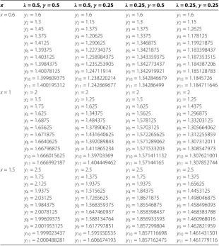
Table 4 The solutions obtained by the new modified Ishikawa iteration method for different
values of
λ
and
γ
x λ= 0.5,γ= 0.5 λ= 0.5,γ= 0.25 λ= 0.25,γ= 0.5 λ= 0.25,γ= 0.25 x= 0.6 y1= 1.6
y2= 1.3
y3= 1.45
y4= 1.375
y5= 1.4125
y6= 1.39375
y7= 1.403125
y8= 1.3984375
y9= 1.40078125
y10= 1.399609375
y11= 1.400195312
y1= 1.6
y2= 1.15
y3= 1.375
y4= 1.20625
y5= 1.290625
y6= 1.22734375
y7= 1.258984375
y8= 1.235253905
y9= 1.24711914
y10= 1.238220214
y11= 1.242669677
y1= 1.6
y2= 1.3
y3= 1.375
y4= 1.3375
y5= 1.346875
y6= 1.3421875
y7= 1.343359375
y8= 1.342773437
y9= 1.342919921
y10= 1.342846679
y11= 1.34286499
y1= 1.6
y2= 1.15
y3= 1.2625
y4= 1.178125
y5= 1.19921875
y6= 1.183398437
y7= 1.187353515
y8= 1.184387206
y9= 1.185128783
y10= 1.1845726
y11= 1.184711646
x= 1 y1= 2
y2= 1.5
y3= 1.75
y4= 1.625
y5= 1.6875
y6= 1.65625
y7= 1.671875
y8= 1.6640625
y9= 1.66796875
y10= 1.666015625
y11= 1.666992187
y1= 2
y2= 1.25
y3= 1.625
y4= 1.34375
y5= 1.484375
y6= 1.37890625
y7= 1.431640625
y8= 1.392089843
y9= 1.411865234
y10= 1.39703369
y11= 1.404449462
y1= 2
y2= 1.5
y3= 1.625
y4= 1.5625
y5= 1.578125
y6= 1.5703125
y7= 1.572265625
y8= 1.571289062
y9= 1.571533203
y10= 1.571411132
y11= 1.57144165
y1= 2
y2= 1.25
y3= 1.4375
y4= 1.296875
y5= 1.33203125
y6= 1.305664062
y7= 1.312255859
y8= 1.307312011
y9= 1.308547973
y10= 1.307621001
y11= 1.307852744
x= 1.5 y1= 2.5
y2= 1.75
y3= 2.125
y4= 1.9375
y5= 2.03125
y6= 1.984375
y7= 2.0078125
y8= 1.99609375
y9= 2.001953125
y10= 1.999023437
y11= 2.000488281
y1= 2.5
y2= 1.375
y3= 1.9375
y4= 1.515625
y5= 1.7265625
y6= 1.568359375
y7= 1.647460937
y8= 1.588134764
y9= 1.617797851
y10= 1.595550535
y11= 1.606674193
y1= 2.5
y2= 1.75
y3= 1.9375
y4= 1.84375
y5= 1.8671875
y6= 1.85546875
y7= 1.858398437
y8= 1.856933593
y9= 1.857299804
y10= 1.857116698
y11= 1.857162475
y1= 2.5
y2= 1.375
y3= 1.65625
y4= 1.4453125
y5= 1.498046875
y6= 1.458496093
y7= 1.468383788
y8= 1.460968016
y9= 1.462821959
y10= 1.461431501
y11= 1.461779116
Table 5 Absolute error of Example 2.1 for different values of
λ
and
γ
(
x
= 0.2,
x
= 0.4 and
x
= 0.6 respectively)
x= 0.2 x= 0.4 x= 0.6
λ
= 0.5,γ
= 0.5 0.12398437 0.173203126 0.289804688λ
= 0.5,γ
= 0.25 0.129110108 0.278220216 0.447330323λ
= 0.25,γ
= 0.5 0.09571167 0.21142334 0.34713501λ
= 0.25,γ
= 0.25 0.148429452 0.316858903 0.505288354λ
= 0.75,γ
= 0.25 0.090887414 0.201774827 0.33266224λ
= 0.25,γ
= 0.75 0.049999962 0.119999924 0.209999886λ
= 0.75,γ
= 0.75 0.02541195 0.070823899 0.136235849Picard 0.0003 0.002328 0.007369875
Runge-Kutta 0.000000435 0.000000081 0.00000046
Euler 0.01 0.020910977 0.032659931
y
= .x
,
y
= .x
,
y
= .x
,
are found and also for
λ
= .,
γ
= .,
y
=
x
,
y
= .x
,
y
= .x
,
y
= .x
,
y
= .x
,
y
= .x
,
y
= .x
,
y
= .x
,
y
= .x
,
y
= .x
,
y
= .x
are obtained. On the other hand, for
λ
= .,
γ
= .,
y
=
x
,
y
=
x
,
y
= .x
,
y
= .x
,
y
= .x
,
y
= .x
,
y
= .x
,
y
= .x
,
y
= .x
,
y
= .x
,
y
= .x
are calculated. In the same way, for
λ
= .,
γ
= .,
y
=
x
,
y
= .x
,
y
= .x
,
y
= .x
,
y
= .x
,
y
= .x
,
y
= .x
,
y
= .x
,
y
= .x
,
y
= .x
are found and also for
λ
= .,
γ
= .,
y
=
x
,
y
= .x
,
y
= .x
,
y
= .x
,
y
= .x
,
y
= .x
,
y
= .x
,
y
= .x
,
y
= .x
,
y
= .x
,
y
= .x
are obtained. Similarly, for
λ
= .,
γ
= .,
y
=
x
,
y
= .x
,
y
= .x
,
y
= .x
,
y
= .x
,
y
= .x
,
y
= .x
,
y
= .x
,
y
= .x
,
y
= .x
,
are calculated. Finally, for
λ
= .,
γ
= .,
y
=
x
,
y
= .x
,
y
= .x
,
y
= .x
,
y
= .x
,
y
= .x
,
y
= .x
,
y
= .x
,
y
= .x
,
y
= .x
,
y
= .x
are found. Now, we get the approximate solution using by the Euler method. Firstly, we
use the formula
y
n+=
y
n+
hF(x
n,
y
n)
with
F(x,
y) =
y
+
x
,
h
= . and
x
= ,
y
= . From the initial condition
y() = , we have
F(, ) = . We now proceed with the calculations as follows:
y
=
y
+
hF(y
,
x
) = + . = .,
x
=
x
+
h
= . + . = .,
y
=
y
+
hF(y
,
x
) = . + .
·
. = .,
x
=
x
+
h
= . + . = .,
y
=
y
+
hF(y
,
x
) = . + . = .,
x
=
x
+
h
= . + . = ..
Finally, applying the Runge-Kutta method to the given initial value problem, we carry out
the intermediate calculations in each step to give figures after decimal point and round
off the final results each at step to four such places.
F(x,
y) =
y
+
x
,
x
= ,
y
= and we
are to use
h
= .. Using these quantities, we calculated successively
k
,
k
,
k
,
k
and
K
defined by
k
=
hg(y
,
x
),
k
=
hg
y
+
h
,
x
+
k
k
=
hg
y
+
h
,
x
+
k
,
k
=
hg(y
+
h,
x
+
k
)
and
K
=
(k
+ k
+ k
+k
),
y
n+=
y
n+
K
. Thus we find
k
,
k
,
k
,
k
for
n
= as follows:
k
= .f
(x
,
y
) = ,
k
= .f
x
+ .,
y
+
k
= .,
k
= .f
x
+ .,
y
+
k
= .,
k
= .f
(x
+ .,
y
+
k
) = ..
So,
y
= . is obtained for
x
= .. On the other hand, we calculated
k
,
k
,
k
,
k
for
n
= as follows:
k
= .f
(x
,
y
) = .,
k
= .f
x
+ .,
y
+
k
= .,
k
= .f
x
+ .,
y
+
k
= .,
k
= .f
(x
+ .,y
+
k
) = ..
Hence
y
= . is calculated for
x
= .. Finally, we get
k
,
k
,
k
,
k
for
n
= as follows:
k
= .f
(x
,
y
) = .,
k
= .f
x
+ .,
y
+
k
= .,
k
= .f
x
+ .,
y
+
k
= .,
k
= .f
(x
+ .,
y
+
k
) = ..
Thus
y
= . is obtained for
x
= ..
After the necessary calculation which is done above, the comparison is shown
schemat-ically in Figure .
On the other hand, we may give Table , Table , Table and Table by the new modified
Ishikawa iteration method for different values of
λ
and
γ
. Now we may give Table which
is expressed that absolute error of Example . for different values of
λ
and
γ
with
x
= .,
x
= . and
x
= . respectively.
Figure 2 The comparison of exact solution and approximate solution of Example 2.2 for different values of
λ
andγ
.The best approximation is obtained taking the different values of
λ
and
γ
and using the
modified Ishikawa iteration method for x
= .,
x
= .
and x
= .
getting
(
λ
= .,
γ
=
.;
λ
= .,
γ
= .;
λ
= .,
γ
= .;
λ
= .,
γ
= .;
λ
= .,
γ
= .;
λ
= .,
γ
= .;
λ
= .,
γ
= .)
respectively.
Similarly,
we calculated the solution for x
= .,
x
=
and x
= .
then the approximation
is found more sensitive taking
(
λ
= .,
γ
= .;
λ
= .,
γ
= .;
λ
= .,
γ
= .;
λ
= .,
γ
= .;
λ
= .,
γ
= .;
λ
= .,
γ
= .;
λ
= .,
γ
= .)
respectively.
Corollary .
Absolute error of the modified Ishikawa iteration method is computed
tak-ing different values of
λ
and
γ
(x
= .,
x
= .
and x
= .),
which is not more effective than
Picard,
Runge-Kutta and Euler iteration methods.
Example .
Let us consider the differential equation
y
= x(y
+ )
subject to the initial condition
y() = .
Using Theorem . and Corollary ., since
T
=
xx
F(t,
y
n(t))dt, then
T
has a unique fixed
Table 6 The solutions obtained by the new modified Ishikawa iteration method for different
values of
λ
and
γ
x λ= 0.5,γ= 0.5 λ= 0.5,γ= 0.25 λ= 0.25,γ= 0.5 λ= 0.25,γ= 0.25 x= 0.2 y1= 0.002666666667
y2= 0.0013333
y3= 0.002
y4= 0.001666664
y5= 0.0018333328
y6= 0.001749999864
y7= 0.001791666568
y8= 0.001770833216
y9= 0.001781249888
y10= 0.001776041312
y11= 0.00177864572
y1= 0.002666666667
y2= 0.00066666664
y3= 0.00166666528
y4= 0.00091666432
y5= 0.00129166648
y6= 0.00101041644
y7= 0.001151041456
y8= 0.001045572688
y9= 0.001098307072
y10= 0.00105875628
y11= 0.001078531672
y1= 0.002666666667
y2= 0.001333333333
y3= 0.001666666664
y4= 0.001499999992
y5= 0.001541666664
y6= 0.001520833328
y7= 0.001526041656
y8= 0.001523437488
y9= 0.001522786448
y10= 0.001523111968
y11= 0.001523030584
y1= 0.002666666667
y2= 0.000666666664
y3= 0.001166666666
y4= 0.000791666664
y5= 0.000885416664
y6= 0.00081510416
y7= 0.00083268228
y8= 0.000819498688
y9= 0.000822794584
y10= 0.000820322656
y11= 0.00082094064
x= 0.4 y1= 0.021333333
y2= 0.010666666
y3= 0.016
y4= 0.013333333
y5= 0.014666662
y6= 0.013999998
y7= 0.014333332
y8= 0.014166665
y9= 0.014249999
y10= 0.014208332
y11= 0.014229165
y1= 0.021333333
y2= 0.00533333312
y3= 0.013333332
y4= 0.007333331456
y5= 0.010333333
y6= 0.00808333152
y7= 0.009208331648
y8= 0.008364581504
y9= 0.008786456576
y10= 0.00847005024
y11= 0.008628253376
y1= 0.021333333
y2= 0.010666666
y3= 0.013333333
y4= 0.011999999
y5= 0.012333333
y6= 0.012166666
y7= 0.012208333
y8= 0.012187499
y9= 0.012182291
y10= 0.012184895
y11= 0.012184244
y1= 0.021333333
y2= 0.00533333312
y3= 0.009333333331
y4= 0.006333333312
y5= 0.007083333312
y6= 0.00652083328
y7= 0.00666145824
y8= 0.006555989504
y9= 0.006582356672
y10= 0.006562581248
y11= 0.00656752512
x= 0.5 y1= 0.041666666
y2= 0.020833333
y3= 0.03125
y4= 0.026041625
y5= 0.028645825
y6= 0.027343747
y7= 0.02799479
y8= 0.027669269
y9= 0.027832029
y10= 0.027750649
y11= 0.027791339
y1= 0.041666666
y2= 0.010416666
y3= 0.026041664
y4= 0.014322913
y5= 0.020182288
y6= 0.015787756
y7= 0.017985022
y8= 0.016337073
y9= 0.017161048
y10= 0.016543066
y11= 0.016852057
y1= 0.041666666
y2= 0.020833333
y3= 0.026041666
y4= 0.023437499
y5= 0.024088541
y6= 0.02376302
y7= 0.0238444
y8= 0.02380371
y9= 0.023793538
y10= 0.023798624
y11= 0.023797352
y1= 0.041666666
y2= 0.010416666
y3= 0.018229166
y4= 0.012369791
y5= 0.013834635
y6= 0.012736025
y7= 0.01301066
y8= 0.012804667
y9= 0.012856165
y10= 0.012817541
y11= 0.012827197
Firstly, we obtained the exact solution of the equation as
y
=
e
x– . Then we approach
the approximate solution by the Picard iteration method as follows:
y
=
x
,
y
=
x
+
x
,
y
=
x
+
x
+
x
,
y
=
x
+
x
!
+
x
!
+
x
!
.
Now, applying the new modified Ishikawa iteration method to the equation for
λ
= .,
γ
= ., then
y
=
x
,
y
= .x
,
Table 7 The solutions obtained by the new modified Ishikawa iteration method for different
values of
λ
and
γ
x λ= 0.75,γ= 0.25 λ= 0.25,γ= 0.75 λ= 0.75,γ= 0.75 x= 0.2 y1= 0.002666666667
y2= 0.000666666664
y3= 0.002166666664
y4= 0.001041666664
y5= 0.001885416664
y6= 0.00125260416
y7= 0.001727213536
y8= 0.001371256504
y9= 0.001638224272
y10= 0.00143799844
y11= 0.001588167816
y1= 0.002666666667
y2= 0.002
y3= 0.002166666664
y4= 0.002125
y5= 0.002135416664
y6= 0.002132812496
y7= 0.002133463536
y8= 0.002133300776
y9= 0.002133341464
y10= 0.002133331288
y11= 0.002133333832
y1= 0.002666666667
y2= 0.002
y3= 0.0025
y4= 0.002375
y5= 0.00246875
y6= 0.002445312496
y7= 0.002462890624
y8= 0.002458496088
y9= 0.002461791984
y10= 0.002406096801
y11= 0.002461585992
x= 0.4 y1= 0.021333333
y2= 0.005333333312
y3= 0.017333333
y4= 0.008333333312
y5= 0.015083333
y6= 0.010020833
y7= 0.0138177708
y8= 0.010970052
y9= 0.013105794
y10= 0.011503987
y11= 0.012705342
y1= 0.021333333
y2= 0.016
y3= 0.017333333
y4= 0.017
y5= 0.017083333
y6= 0.017062499
y7= 0.017067708
y8= 0.017066406
y9= 0.017066731
y10= 0.01706665
y11= 0.01706667
y1= 0.021333333
y2= 0.016
y3= 0.02
y4= 0.019
y5= 0.01975
y6= 0.019562499
y7= 0.019703124
y8= 0.019667968
y9= 0.019694335
y10= 0.019687744
y11= 0.019692687
x= 0.5 y1= 0.041666666
y2= 0.010416666
y3= 0.033854166
y4= 0.016276041
y5= 0.029459635
y6= 0.01957194
y7= 0.026987711
y8= 0.021425882
y9= 0.025597254
y10= 0.022468725
y11= 0.024815122
y1= 0.041666666
y2= 0.03125
y3= 0.033854166
y4= 0.033203125
y5= 0.033365885
y6= 0.033325195
y7= 0.033335367
y8= 0.033335367
y9= 0.03333346
y10= 0.033333301
y11= 0.033333341
y1= 0.041666666
y2= 0.03125
y3= 0.0390625
y4= 0.037109375
y5= 0.038574218
y6= 0.038208007
y7= 0.038482666
y8= 0.038414001
y9= 0.038465499
y10= 0.038452625
y11= 0.038462281