Adaptive Geometric Multiscale Approximations for
Intrinsically Low-dimensional Data
Wenjing Liao [email protected]
School of Mathematics
Georgia Institute of Technology, Atlanta, GA, 30313, USA
Mauro Maggioni [email protected]
Department of Mathematics, Department of Applied Mathematics and Statistics, Johns Hopkins University, 3400 N. Charles Street, Baltimore, MD 21218, USA
Editor:Sujay Sanghavi
Abstract
We consider the problem of efficiently approximating and encoding high-dimensional data sampled from a probability distributionρinRD, that is nearly supported on ad-dimensional
setM- for example supported on ad-dimensional manifold. Geometric Multi-Resolution Analysis (GMRA) provides a robust and computationally efficient procedure to construct low-dimensional geometric approximations of M at varying resolutions. We introduce GMRA approximations that adapt to the unknown regularity of M, by introducing a thresholding algorithm on the geometric wavelet coefficients. We show that these data-driven, empirical geometric approximations perform well, when the threshold is chosen as a suitable universal function of the number of samples n, on a large class of measuresρ, that are allowed to exhibit different regularity at different scales and locations, thereby efficiently encoding data from more complex measures than those supported on manifolds. These GMRA approximations are associated to a dictionary, together with a fast transform mapping data tod-dimensional coefficients, and an inverse of such a map, all of which are data-driven. The algorithms for both the dictionary construction and the transforms have complexityCDnlognwith the constantCexponential ind. Our work therefore establishes Adaptive GMRA as a fast dictionary learning algorithm, with approximation guarantees, for intrinsically low-dimensional data. We include several numerical experiments on both synthetic and real data, confirming our theoretical results and demonstrating the effective-ness of Adaptive GMRA.
Keywords: Dictionary Learning, Multi-Resolution Analysis, Adaptive Approximation, Manifold Learning, Compression
1. Introduction
We model a data set as n i.i.d. samples Xn := {xi}ni=1 from a probability measure ρ in
RD. We make the assumption that ρis supported on or near a setMof dimensiondD,
and consider the problem, givenXn, of learning a data-dependent dictionary that enables
c
efficient encoding of (future) data sampled from ρ, together with fast forward and inverse transforms between RD and the space of encodings.
In order to circumvent the curse of dimensionality, a popular model for data is sparsity: we say that the data is k-sparse on a suitable dictionary (i.e. a collection of vectors) Φ =
{ϕi}mi=1 ⊂RD if each data pointx∈Rdmay be expressed as a linear combination of at most
k elements of Φ. Clearly the case of interest isk D. Thesesparse representations have been used in a variety of statistical signal processing tasks, compressed sensing, machine learning (see e.g. Protter and Elad, 2007; Peyr´e, 2009; Lewicki et al., 1998; Kreutz-Delgado et al., 2003; Maurer and Pontil, 2010; Chen et al., 1998; Donoho, 2006; Aharon et al., 2005; Candes and Tao, 2007, among many others), and spurred much research about how to learn data-driven dictionaries (see Gribonval et al., 2015; Vainsencher et al., 2011; Maurer and Pontil, 2010, and references therein). The algorithms used in dictionary learning are often computationally demanding, and based on high-dimensional non-convex optimization (Mairal et al., 2010). These approaches have the strength of being very general, with minimal assumptions on the geometry of the dictionary or on the distribution from which the samples are generated. This “worst-case” approach incurs bounds depending upon the ambient dimensionDin general (even in the standard case of data lying on one hyperplane). It is possible to tackle the dictionary learning problem under geometric assumptions on data sets (Maggioni et al., 2016), namely that data lie on or near a low-dimensional set
M. There are of course various possible geometric assumptions, the simplest one being that M is a single d-dimensional subspace, in which case Principal Component Analysis (PCA) (see Pearson, 1901; Hotelling, 1933, 1936) suffices for estimating the subspace. More generally, one may assume that data lie on a union of several low-dimensional planes instead of a single one. The problem of estimating multiple planes, called subspace clustering, is more challenging (see Fischler and Bolles, 1981; Ho et al., 2003; Vidal et al., 2005; Yan and Pollefeys, 2006; Ma et al., 2007, 2008; Chen and Lerman, 2009; Elhamifar and Vidal, 2009; Zhang et al., 2010; Liu et al., 2010; Chen and Maggioni, 2011). This model was shown effective in various applications, including image processing (Fischler and Bolles, 1981), computer vision (Ho et al., 2003) and motion segmentation (Yan and Pollefeys, 2006). Yet another type of geometric model gives rise to manifold learning, where M is assumed to
be a d-dimensional manifold isometrically embedded in RD, see (Tenenbaum et al., 2000;
Roweis and Saul, 2000; Belkin and Niyogi, 2003; Donoho and Grimes, 2003; Coifman et al., 2005a,b; Zhang and Zha, 2004) and many others. It is of interest to move beyond this model to even more general geometric models, for example where the regularity of the manifold is reduced, and data are not forced to lie exactly on a manifold, but only close to it.
directions. At a fixed scaleMis thereby approximated by a piecewise linear set. In Allard et al. (2012) the performance of GMRA for volume measures on aCs, s∈(1,2] manifold was
analyzed in the continuous case (i.e. with no sampling), albeit the effectiveness of GMRA was demonstrated empirically on simulated and real-world data, but for a fixed data set, and without out-of-sample extension. In Maggioni et al. (2016), the approximation error of M was estimated in the non-asymptotic regime with n i.i.d. samples from a measure
ρ, satisfying certain technical assumptions, supported on a thin tube of a C2 manifold of
dimension d isometrically embedded in RD. The concentration bounds in Maggioni et al.
(2016) depend on nand d, but not on D, successfully avoiding the curse of dimensionality caused by the ambient dimension. The assumption that ρ is supported in a tube around a manifold can account for noise and does not force the data to lie exactly on a smooth low-dimensional manifold.
In both Allard et al. (2012) and Maggioni et al. (2016), GMRA approximations are con-structed on uniform partitions, at a fixed scale, in which all the cells have similar diameters. However, when the regularity of M, such as smoothness or curvature, weighted by the ρ measure, varies at different scales and locations, uniform partitions do not yield optimal approximations. Inspired by the adaptive methods in classical multi-resolution analysis of functions (see Donoho and Johnstone, 1994, 1995; Cohen et al., 2002; Binev et al., 2005, 2007, among many others, and references therein), we propose an adaptive version of GMRA to construct low-dimensional geometric approximations ofMon an adaptive partition, and provide finite sample performance guarantees for a larger classes of geometric structuresM than those considered in Maggioni et al. (2016). This truly takes advantage of the multiscale structure of GMRA, and leads to simple yet provably powerful approximations for a large class of geometric objects that are not necessarily equally regular at all scales and locations. Our main result (Theorem 8) in this paper may be paraphrased as follows: Let ρ be a probability measure supported on or near a compactd-dimensional manifoldM,→RD, with
d≥3. Assume thatρadmits a(n unknown) multiscale decomposition satisfying the techni-cal assumptions A1-A5 in section 2.1. Givenni.i.d. samples ofρ, the intrinsic dimensiond, and a parameterκ large enough, Adaptive GMRA outputs a dictionary Φbn={φbi}i∈Jn, an encoding operatorDbn:RD →R(d+1)Jn and a decoding operatorDbn−1 :R(d+1)Jn →RDthat,
with high probability, satisfy the following properties. For every x ∈RD, kDbnxk0 ≤d+ 1
(i.e. only d+ 1 entries of the encoded data are non-zero), and the Mean Squared Error (MSE), over data sampled from ρ, satisfies
MSE :=Ex∼ρ[kx−Dbn−1Dbnxk2].
logn n
2s
2s+d−2
.
Heresis a regularity parameter ofρ(as in definition 5), which allows us to considerM’s and
ρ’s with nonuniform regularity, varying at different locations and scales. The parameterκis
used in choosing the threshold on the geometric wavelet coefficients, and selecting from the GMRA a multiscale partition and set of local approximate tangent planes to use for encoding the data. Note that the algorithm does not need to know s (indeed, κ is independent of
s), but it automatically adapts to obtain a rate that depends on s. We believe, but do not
prove, that this rate is indeed optimal. As for computational complexity, constructing Φbn
takesO((Cd+d2)Dnlogn) and computingDbnxonly takesO(d(D+d2) logn), which means
In Adaptive GMRA, the dictionary is composed of the low-dimensional planes on adap-tive partitions and the encoding operator transforms a point to the local affined+1 principal coefficients of the data in a piece of the partition (the first affine principal component here means the local mean). We state this results in terms of encoding and decoding to stress that learning the geometry in fact yields efficient representations of data, which may be used for performing signal processing tasks in a domain where the data admit a sparse representation, e.g. in compressive sensing or estimation problems (see Iwen and Maggioni, 2013; Chen et al., 2012; Eftekhari and Wakin, 2015). Adaptive GMRA is designed towards robustness, both in the sense of tolerance to noise and to model error (i.e. data not lying on a manifold). We assumedis given throughout this paper. If not, we refer to Little et al. (2017, 2009a,b) for the estimation of intrinsic dimensionality.
The paper is organized as follows. Our main results, including the construction of GMRA, Adaptive GMRA and their finite sample analysis, are presented in Section 2. We show numerical experiments in Section 3. The detailed analysis of GMRA and Adaptive GMRA is presented in Section 4. In Section 5, we discuss the computational complexity of Adaptive GMRA and extend our work to adaptive orthogonal GMRA. Proofs are collected in the appendix.
Notation. We will introduce some basic notation here. f . g means that there exists a constant C independent on any variable upon which f and g depend, such that f ≤ Cg; similarly for &. f g means that f .g and f &g. The cardinality of a set A is denoted by #A. Forx∈RD,kxkdenotes the Euclidean norm andBr(x) denotes the Euclidean ball
of radius r centered at x. Given a subspace V ∈RD, we denote its dimension by dim(V)
and the orthogonal projection ontoV by ProjV. IfAis a linear operator onRD,||A|| is its
operator norm. The identity operator is denoted byI.
2. Main results
GMRA was proposed in Allard et al. (2012) to efficiently represent points on or near a low-dimensional manifold in high dimensions. We refer the reader to that paper for details of the construction, and we summarize here the main ideas in order to keep the presentation self-contained. The construction of GMRA involves the following steps:
(i) construct amultiscale tree T and the associated decomposition ofMinto nested cells
{Cj,k}k∈Kj,j∈Z where j represents scale andklocation;
(ii) performlocal PCAon eachCj,k: let the mean (“center”) becj,kand thed-dim principal
subspaceVj,k. Define Pj,k(x) :=cj,k+ ProjVj,k(x−cj,k).
(iii) construct a “difference” subspace Wj+1,k0 capturing Pj,k(Cj,k)− Pj+1,k0(Cj+1,k0), for
each Cj+1,k0 ⊆Cj,k (these quantities are associated with the refinement criterion in
Adaptive GMRA).
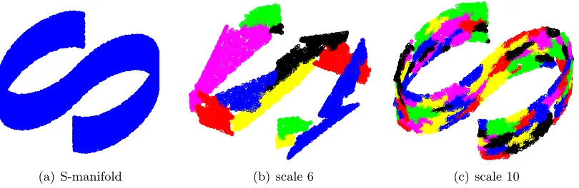
(a) S-manifold
j = 6
(b) scale 6
j = 10
(c) scale 10
Figure 1: (a) S-manifold; (b,c) Linear approximations at scale 6,10.
unknown, and the construction above is carried over on training data, and its result is ran-dom with respect to the training samples. Naturally we are interested in the performance of the construction on new samples. This is analyzed in a setting of “smooth manifold+noise” in Maggioni et al. (2016). When the regularity (such as smoothness or curvature) of M varies at different locations and scales, linear approximations on fixed uniform partitions are not optimal. Inspired by adaptive methods in classical multi-resolution analysis (see Cohen et al., 2002; Binev et al., 2005, 2007), we propose an adaptive version of GMRA which learns adaptive and near-optimal approximations.
We will start with the multiscale tree decomposition in Section 2.1 and present GMRA and Adaptive GMRA in Section 2.3 and 2.4 respectively.
2.1. Multiscale partitions and trees
A multiscale set of partitions of M with respect to the probability measure ρ is a family of sets {Cj,k}k∈Kj,j∈Z, called dyadic cells, satisfying Assumptions (A1-A5) below, for all
integers j≥jmin:
(A1) for any k ∈ Kj and k0 ∈ Kj+1, either Cj+1,k0 ⊆ Cj,k or ρ(Cj+1,k0 ∩Cj,k) = 0. We
denote the children ofCj,k by C(Cj,k) = {Cj+1,k0 :Cj+1,k0 ⊆Cj,k}. We assume that
amin ≤ #C(Cj,k) ≤amax. Also for every Cj,k, there exists a unique k0 ∈ Kj−1 such
thatCj,k ⊆Cj−1,k0. We callCj−1,k0 the parent ofCj,k.
(A2) ρ(M \ ∪k∈KjCj,k) = 0, i.e. Λj :={Cj,k}k∈Kj is a cover for M.
(A3) ∃θ1 >0 : #Λj ≤2jd/θ1.
(A4) ∃θ2 >0 such that, if xis drawn from ρ|Cj,k, then a.s. kx−cj,kk ≤θ22−j.
(A5) Let λj,k1 ≥λj,k2 ≥. . .≥λj,kD be the eigenvalues of the covariance matrix Σj,k ofρ|Cj,k,
defined in Table 1. Then:
(i) ∃θ3>0 such that∀j≥jmin and k∈ Kj,λj,kd ≥θ32−2j/d,
(A1) implies that the{Cj,k}k∈Kj,j≥jmin are associated with a tree structure, and with some
abuse of notation we call the abovetree decompositions. (A1)-(A5) are natural assumptions, easily satisfied by natural multiscale decompositions when Mis a d-dimensional manifold isometrically embedded inRD: see the work (Maggioni et al., 2016) for a detailed discussion,
where the connections between the constantsθi’s and geometric properties ofM(curvatures,
reach, etc...) are also discussed. (A2) guarantees that the cells at scalej form a partition of
M; (A3) says that there are at most 2jd/θ1dyadic cells at scalej. (A4) ensures diam(Cj,k).
2−j. When M is a d-dimensional manifold, (A5)(i) is the condition that the best rank d
approximation to Σj,k is close to the covariance matrix of a d-dimensional Euclidean ball,
while (A5)(ii) imposes that the (d+ 1)-th eigenvalue is smaller that thed-th eigenvalue, i.e. the set has significantly larger variances inddirections than in all the remaining ones. The conditions generalize those in (Allard et al., 2012) (which corresponded to the case when
Mis a manifold) and in (Maggioni et al., 2016), for example by not assuming that all sets
{Cj,k}k (for any fixedj) have roughly the same volume, and also by weakening (A5). These
changes enlarge the class of measures ρ and sets M that we consider here, for exampling allowing for a highly nonuniform measureρ, and an Msubstantially “thickened” in many dimensions.
We will construct such {Cj,k}k∈Kj,j≥jmin in Section 2.6. In our construction (A1-A4)
is satisfied when ρ is a regular doubling probability measure1 (see Christ, 1990; Deng and Han, 2008). If we further assume thatM is a d-dimensional Cs, s∈(1,2] closed manifold isometrically embedded inRD, then (A5) is satisfied as well (See Proposition 14).
It may happen that at the coarsest scales conditions (A3)-(A5) are satisfied but with very poor constantsθ: it will be clear that in all that follows we may discard a few coarse scales (i.e. by enlarging jmin), and only work at scales that are fine enough and for which
(A3)-(A5) truly capture the local geometry of M.
Some notation: a master tree T is associated with {Cj,k}k∈Kj,j≥jmin (using property
(A1)), constructed on M; since Cj,k’s at scale j have similar diameters, Λj := {Cj,k}k∈Kj is called auniform partition at scale j. A proper subtree ˜T of T is a collection of nodes of
T with the properties: (i) the root node is in ˜T, (ii) if Cj,k is in ˜T then the parent of Cj,k
is also in ˜T. Any finite proper subtree ˜T is associated with a unique partition Λ = Λ( ˜T) which consists of its outer leaves, by which we mean thoseCj,k ∈ T such thatCj,k ∈/T˜ but
its parent is in ˜T.
2.2. Empirical GMRA
In practice the master tree T is not given, nor can be constructed since M is not known: we will construct one on samples by running a variation of the cover tree algorithm (see Beygelzimer et al., 2006), which only creates candidate “centers” for theCj,k, by adding a
multiscale partitioning step. From now on we denote the training data byX2n. We randomly
split the data into two disjoint groups such thatX2n=Xn0∪XnwhereXn0 ={x01, . . . , x0n}and
Xn= {x1, . . . , xn}, apply our variation on cover trees onXn0 to construct a tree satisfying
(A1-A5) (see section 2.6). After the tree is constructed, we assign points in the second
1.ρis regular doubling if there existsC1>0 such thatC1−1r d≤
ρ(M ∩Br(x))≤C1rdfor anyx∈ Mand
GMRA Empirical GMRA Linear projection
onCj,k Pj,k(x) :=cj,k+ ProjVj,k(x−cj,k) Pbj,k(x) :=bcj,k+ ProjVbj,k(x−bcj,k)
Linear projection
at scalej Pj:= P
k∈KjPj,k1j,k Pbj:=
P
k∈KjPbj,k1j,k
Measure ρ(Cj,k) ρb(Cj,k) =nbj,k/n
Center cj,k:=Ej,kx bcj,k:= bn1j,k P
xi∈Cj,kxi
Principal subspaces
Vj,kminimizes Ej,kkx−cj,k−ProjV(x−cj,k)k2
amongd-dim subspaces
b
Vj,kminimizes
1
b nj,k
P
xi∈Cj,kkx−bcj,k−ProjV(x−bcj,k)k 2
amongd-dim subspaces Covariance
matrix Σj,k:=Ej,k(x−cj,k)(x−cj,k)
T Σb
j,k:= bn1j,kPxi∈Cj,k(xi−bcj,k)(xi−bcj,k)
T
Inner product
with respect toρ hPX,QXi:= ´
MhPx,Qxidρ 1/n
P
xi∈XnhPxi,Qxii
Norm with
respect toρ kPXk:= ´
MkPxk2dρ
1
2 1/nP
xi∈XnkPxik
212
Table 1: This table summarizes GMRA-related quantities and their empirical counterparts (Allard et al., 2012; Maggioni et al., 2016). 1j,k is the indicator function on Cj,k
(i.e.,1j,k(x) = 1 ifx∈Cj,k and 0 otherwise). HereEj,k stands for expectation with
respect to the conditional distributiondρ|
Cj,k. The measure ofCj,k is ρ(Cj,k) and the empirical measure is ρ(Cb j,k) = bnj,k/n where bnj,k is the number of points in
Cj,k. Vj,k and Vbj,k are the eigen-spaces associated with the largest d eigenvalues
of Σj,k and Σbj,k respectively. HereP,Q: M →RD are two operators.
half of data Xn, to the appropriate cells. In this way we obtain a family of multiscale
partitions for the points in Xn, which we truncate to the largest subtree whose leaves
contain at least d points in Xn. This subtree is called the data master tree, denoted by
Tn. We then use Xn to perform local PCA to obtain the empirical mean bcj,k and the
empiricald-dimensional principal subspaceVbj,kon eachCj,k. Define the empirical projection b
Pj,k(x) := bcj,k + ProjVbj,k(x−bcj,k) for x ∈ Cj,k. Table 1 summarizes the GMRA-related quantities and their empirical counterparts.
2.3. Geometric Multi-Resolution Analysis: uniform partitions
GMRA with respect to the distribution ρ associated with the multiscale tree T consists a collection of piecewise affine projectors {Pj : RD → RD}j≥jmin on the multiscale
par-titions {Λj := {Cj,k}k∈Kj}j≥jmin. At scale j, M is approximated by the piecewise
linear sets {Pj,k(Cj,k)}k∈Kj. The approximation error of M by the empirical linear sets
{Pbj,k(Cj,k)}k∈Kj is defined as:
EkX−PbjXk2=E
ˆ
Mk
x−Pbjxk2dρ=E
X
k∈Kj
ˆ
Cj,k
where Pbj and Pbj,k are built from random samples xi ∼ ρ (according to the GMRA
algo-rithm),X is a random vector distributed according to ρ, and the expectation is taken over X. The squared approximation error above is also called the Mean Square Error (MSE) of GMRA. In order to understand the error, we split it into a bias term and a variance term:
EkX−PbjXk ≤ kX− PjXk
| {z }
bias
+EkPjX−PbjXk
| √ {z }
variance
. (1)
To bound the bias term, we need regularity assumptions on ρ, while for the variance term we prove concentration bounds of the relevant quantities around their expected values.
For a fixed distribution ρ, the approximation error of Mat scale j, measured by kX− PjXk, decays at a rate dependent on the regularity of M in the ρ-measure (see Allard
et al., 2012). We quantify the regularity ofρ as follows:
Definition 1 (Model class As) A probability measure ρ supported onM is inAs if
|ρ|As = sup
T
inf{A0 : kX− PjXk ≤A02−js,∀j≥jmin}<∞, (2)
whereT varies over the set, assumed non-empty, of multiscale tree decompositions satisfying
Assumptions (A1-A5).
We capture the case where theL2 approximation error is roughly the same on every cell with the following definition:
Definition 2 (Model class A∞
s ) A probability measure ρ supported onM is inA∞s if
|ρ|A∞
s = sup
T
inf{A0 : k(X− Pj,kX)1j,kk ≤A02−js
q
ρ(Cj,k), ∀k∈ Kj, j ≥jmin}<∞ (3)
whereT varies over the set, assumed non-empty, of multiscale tree decompositions satisfying
Assumptions (A1-A5).
Clearly A∞s ⊂ As. Also, since diam(Cj,k) ≤ 2θ22−j, necessarily k(I− Pj,k)1j,kXk ≤
θ22−j
p
ρ(Cj,k), ∀k ∈ Kj, j ≥ jmin, and therefore ρ ∈ A∞1 in any case. Moreover, these
classes contain suitable measures supported on manifolds:
Proposition 3 Let M be a closed manifold of class Cs, s∈ (1,2] isometrically embedded
in RD, and ρ be a doubing probability measure onM with the doubling constant C1. Then
our construction of {Cj,k}k∈Kj,j≥jmin in Section 2.6 satisfies (A1-A5), andρ∈ A∞s .
The proof is postponed to Appendix A.2.
Example 1 We consider the d-dim S-manifold whose x1 and x2 coordinates are on an
S-shaped curve andxi ranges in [0,1]for i= 3, . . . , d+ 1. By the Proposition just stated, the
volume measure on this S-manifold is in A∞2 . Numerically one can identify s from data
sampled fromρ∈ As as the slope of the line approximating log10kX− PjXk as a function
of log10rj where rj is the average diameter of Cj,k’s at scalej. Our numerical experiments
scale j
Squared bias Variance
Total error
Optimal scale j*
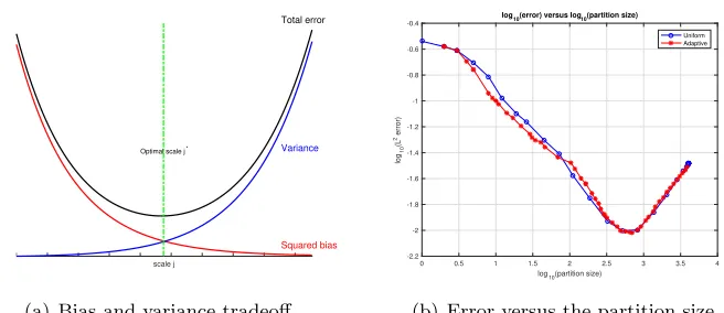
(a) Bias and variance tradeoff
0 0.5 1 1.5 2 2.5 3 3.5 4
log10(partition size)
-2.2 -2 -1.8 -1.6 -1.4 -1.2 -1 -0.8 -0.6 -0.4
log
10
(L
2 error)
log10(error) versus log10(partition size)
Uniform Adaptive
(b) Error versus the partition size
Figure 2: (a) Plot of the bias and variance estimates in Eq. (1), with s = 2, d = 5, n = 100. (b) shows the approximation error on test data versus the partition size in GMRA and Adaptive GMRA for the 3-dim S-manifold. When the partition size is between 1 and 102.8, the bias dominates the error so the error decreases; after that, the variance dominates the error, which becomes increasing.
Example 2 As a comparison we consider the d-dimensional Z-manifold whose x1 and x2
coordinates are on a Z-shaped curve and xi ranges in [0,1], for i = 3, . . . , d+ 1. Volume
measure on the Z manifold is in A1.5 (see appendix B.2). Our numerical experiments in
Figure 5 (c) give rise to s≈1.5,1.7,1.6 when d= 3,4,5 respectively.
The squared bias in (1) satisfieskX−PjXk2 ≤ |ρ|2As2−2jswheneverρ∈ As(by definition
of As). In Proposition 16 we will show that the variance term is estimated in terms of the
sample size nand the scalej as follows:
EkPjX−PbjXk2 ≤
d2#Λ
jlog[αd#Λj]
β22jn =O
j2j(d−2)
n
!
,
whereα, β are constants depending on θ2, θ3. In the case d= 1 both the squared bias and
the variance decrease asjincreases, so choosing the finest scale of the data treeTnyields the best rate of convergence. Whend≥2, the squared bias decreases but the variance increases asj gets large as shown Figure 2, as a manifestation of the classical bias-variance tradeoff, except that it arises here in a geometric setting (a related instance of this phenomenon appears in Canas et al. (2012)). By choosing a proper scalej∗ to balance these two terms, we obtain the following rate of convergence for empirical GMRA truncated at scalej∗:
Theorem 4 Suppose ρ ∈ As for s ≥ 1. Let ν > 0 be arbitrary and fix µ > 0. Let j∗ be chosen such that
2−j∗ =
µlognn for d= 1
µlognn
1 2s+d−2
then there exists C1:=C1(θ1, θ2, θ3, θ4, d, ν, µ) and C2 :=C2(θ1, θ2, θ3, θ4, d, µ) such that:
P
kX−Pbj∗Xk ≥(|ρ|A
sµ
s+C
1)
logn n
≤C2n−ν, for d= 1, (5)
P (
kX−Pbj∗Xk ≥(|ρ|A
sµ
s+C
1)
logn n
s
2s+d−2
)
≤C2n−ν, for d≥2. (6)
Theorem 4 is proved in Section 4.2. From the perspective of dictionary learning, it says that GMRA provides a dictionary Φj∗of cardinalitydn/lognford= 1 andd(n/logn)
d 2s+d−2
ford≥2, consisting of the principal directions in each of theCj∗,k’s (forming the columns
ofVbj∗,x) and the means of theCj∗,k’s, so that everyxsampled fromρ(and not just samples
in the training data) may be encoded with a vector with d+ 1 nonzero entries: one entry encodes the location k of x on the tree, e.g. (j∗, x) = (j∗, k) such that x ∈Cj∗,k, and the
other dentries are the coefficients VbjT∗,x(x−bcj∗,x). We also remind the reader that GMRA
automatically constructs a fast transform mapping pointsx to the vector representing Φj∗
(See Allard et al. (2012); Maggioni et al. (2016) for a discussion). Note that by choosing ν large enough in the Theorem,
(6) =⇒ MSE =EkX−Pbj∗Xk2 .
logn n
2s
2s+d−2
,
and (5) implies MSE .(lognn)2 ford= 1. Clearly, one could fix a desired MSE of size ε2, and obtain a dictionary of size dependent only onεand independent ofn, for nsufficiently large, thereby obtaining a way of compressing data (for further discussion on this point see Maggioni et al. (2016), where also a special case of Theorem 4 withs= 2 was proved).
2.4. Geometric Multi-Resolution Analysis: Adaptive Partitions
The performance guarantee in Theorem 4 is not fully satisfactory for two reasons: (i) the regularity parameter s is required to be known to choose the optimal scale j∗, and this parameter is typically unknown in any practical setting, and (ii) none of the uniform partitions {Cj,k}k∈Kj will be optimal if the regularity of ρ (and/or M) varies at different locations and scales. This lack of uniformity in regularity can appear in a wide variety of data sets for various reasons: when clusters exist that have cores denser than the remaining regions of space, when sampled trajectories of a dynamical system linger in certain regions of space for much longer time intervals than others (e.g. metastable states in molecular
Definition (infinite sample) Empirical version
Difference operator Qj,k := (Pj− Pj+1)1j,k Qbj,k:= (Pbj−Pbj+1)1j,k
Norm of difference ∆2j,k:=´C
j,kkQj,kxk
2dρ ∆b2
j,k:= 1n
P
xi∈Cj,kkQbj,kxik
2
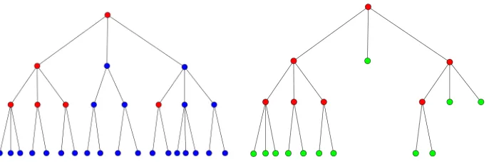
Figure 3: Left: a master tree in which red nodes satisfy ∆j,k ≥2−jτnbut blue nodes do not.
Right: the subtree of the red nodes is the smallest proper subtree that contains all the nodes satisfying ∆j,k ≥2−jτn, i.e. were red in the figure on the left. Green
nodes form the adaptive partition.
dynamics (Rohrdanz et al., 2011; Zheng et al., 2011)), in data sets of images where details exist at different level of resolutions, affecting regularity at different scales in the ambient space, and so on. To fix the ideas we consider again one simplest manifestations of this phenomenon in the examples considered above: uniform partitions work well for the volume measure on the S-manifold but are not optimal for the volume measure on the Z-manifold, for which the ideal partition is coarse on flat regions but finer at and near the corners (see Figure 4). In applications, for example to mesh approximation, it is often the case that the point clouds to be approximated are not uniformly smooth and include different levels of details at different locations and scales (see Figure 9). We therefore propose an adaptive version of GMRA that automatically adapts to the regularity of the data and choose a near-optimal partition.
We expect ∆j,k defined in Table 2 to be small on approximately flat regions, and large
∆j,kat many scales at irregular locations. We also expect∆bj,k to have the same behavior, at
least when ∆bj,k is with high confidence close to ∆j,k. We see this phenomenon represented
in Figure 4 (a,b): as j increases, for the S-manifold kPbj+1xi −Pbjxik decays uniformly
at all points, while for the Z-manifold, the same quantity decays rapidly on flat regions but remains large even at fine scales near the corners (where “near” is scale-dependent, decreasing with scale). We wish to include in our approximation the nodes where this quantity is large, since we may expect a large improvement in approximation by including such nodes. However if too few samples exist in a node, then this quantity is not to be trusted, because its variance is large. It turns out that it is enough to consider the following criterion: let Tbτn be the smallest proper subtree of Tn that contains all Cj,k ∈ Tn for which ∆bj,k ≥2−jτn whereτn=κ
p
(logn)/n. Crucially,κ may be chosen independently of
Algorithm 1 - Adaptive GMRA
Input: dataX2n=Xn0 ∪ Xn, intrinsic dimension d, threshold κ
Output: Tn, {Cj,k}, PbΛbτn : multiscale tree, corresponding cells and adaptive piecewise linear projectors on an adaptive partition.
1: ConstructTn and {Cj,k} from Xn0
2: Now useXn. Compute Pbj,k and ∆bj,k on every nodeCj,k ∈ Tn.
3: Tbτn ← smallest proper subtree of Tn containing all C
j,k ∈ Tn : ∆bj,k ≥ 2−jτn where
τn=κ
p
(logn)/n.
4: Λbτn ← the partition associated with outer leaves ofTbτn
5: PbΛb
τn ←
P
Cj,k∈ΛbτnPbj,k1j,k.
Adaptive partitions may be effectively selected with a criterion that determines whether or not a cell should participate in the adaptive partition. The quantities involved in the selection and their empirical version are summarized in Table 2.
We will provide a finite sample performance guarantee of the empirical Adaptive GMRA for a model class that is more general than A∞s . Given any fixed threshold η > 0, we let
T(ρ,η) be the smallest proper subtree ofT that contains allCj,k∈ T for which ∆j,k ≥2−jη.
The corresponding adaptive partition Λ(ρ,η) consists of the outer leaves of T(ρ,η). We let
#jT(ρ,η) be the number of cells inT(ρ,η) at scalej.
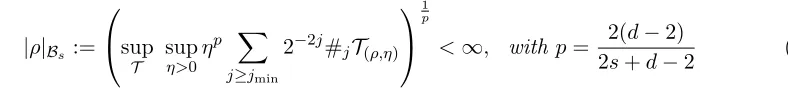
Definition 5 (Model class Bs) In the case d≥3, given s >0, a probability measure ρ
supported onM is in Bs if ρ satisfies the following regularity condition:
|ρ|Bs :=
sup
T
sup
η>0
ηp X
j≥jmin
2−2j#jT(ρ,η)
1 p
<∞, with p= 2(d−2)
2s+d−2 (7)
whereT varies over the set, assumed nonempty, of multiscale tree decompositions satisfying
Assumptions (A1-A5).
For elements in the model class Bs we have control on the growth rate of the truncated
tree T(ρ,η) as η decreases, namely it is O(η−p). Our key estimates on variance and sample
complexity in Lemma 15 indicate that the natural measure of the complexity ofT(ρ,η) is the weighted tree complexity measurePj≥j
min2
−2j#
jT(ρ,η)in the definition above. First of all,
the class Bs is indeed larger than A∞s (see appendix A.4 for a proof):
Lemma 6 Bs is a more general model class than A∞s : if ρ ∈ A∞s , then ρ ∈ Bs and
|ρ|Bs .|ρ|A∞s .
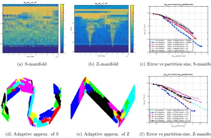
Example 3 The volume measures on the d-dim (d ≥ 3) S-manifold and Z-manifold are
in B2 and B1.5(d−2)/(d−3) respectively (see appendix B). In numerical experiments, s can be
approximated by the negative of the slope in the log-log plot of kX−PbΛbηXk
d−2 versus the
weighted complexity of the truncated tree according to Eq. (9): see numerical examples in
log10||Pj+1x-Pj x||2
1 2 3 4 5 6 7 8 9 10
Point index #104
5
10
15
20
Scale
-10 -8 -6 -4 -2 0 2
(a) S-manifold
log10||Pj+1x-Pj x||2
1 2 3 4 5 6 7 8 9 10 Point index #104
5
10
15
20
25
Scale
-10 -8 -6 -4 -2 0 2
(b) Z-manifold
0 0.5 1 1.5 2 2.5 3 3.5 4 4.5
log10(partition size) -3.5
-3 -2.5 -2 -1.5 -1 -0.5 0
log
10
(L
2 error)
log10error versus log10(partition size)
d=3 Uniform: slope= -0.78825 theory= -0.66667 d=3 Adaptive: slope= -0.76836 theory= -0.66667 d=4 Uniform: slope= -0.59324 theory= -0.5 d=4 Adaptive: slope= -0.61705 theory= -0.5 d=5 Uniform: slope= -0.48404 theory= -0.4 d=5 Adaptive: slope= -0.49943 theory= -0.4
(c) Error vs partition size, S-manifold
(d) Adaptive approx. of S (e) Adaptive approx. of Z
0 0.5 1 1.5 2 2.5 3 3.5 4
log10(partition size) -3.5
-3 -2.5 -2 -1.5 -1 -0.5 0
log
10
(L
2 error)
log10error versus log10(partition size)
d=3 Uniform: slope= -0.58149 theory= -0.5 d=3 Adaptive: slope= -0.77297 theory= -0.75 d=4 Uniform: slope= -0.4914 theory= -0.375 d=4 Adaptive: slope= -0.64198 theory= -0.5 d=5 Uniform: slope= -0.40358 theory= -0.3 d=5 Adaptive: slope= -0.48847 theory= -0.375
(f) Error vs partition size, Z-manifold
Figure 4: (a,b): log10||Pbj(xi)−Pbj+1(xi)|| from the coarsest scale (top) to the finest scale
(bottom), with columns indexed by points, which, for visualization purposes only, are sorted roughly from “left to right” on the manifold. (d,e): adaptive approximations: for the S-manifold the adaptive approximation is close to a uni-form approximation, but for the Z-manifold it contains few large pieces near the almost-flat regions, and several small pieces near the “corners”. (c,f): log-log plot of the approximation error versus the partition size in GMRA and Adap-tive GMRA respecAdap-tively. Theoretically, the slope is −2/d in both GMRA and Adaptive GMRA for the S-manifold. For the Z-manifold, the slope is−1.5/din GMRA and−1.5/(d−1) in Adaptive GMRA (see appendix B).
We also need a quasi-orthogonality condition which says that the operators{Qj,k}k∈Kj,j≥jmin
applied onMare mostly orthogonal across scales and/orkQj,kXk quickly decays.
Definition 7 (Quasi-orthogonality) There exists a constant B0 > 0 such that for any
proper subtree T˜ of any master tree T satisfying Assumptions (A1-A5),
k X
Cj,k∈/T˜
Qj,kXk2 ≤B0
X
Cj,k∈/T˜
kQj,kXk2. (8)
approximation of X by PΛ(ρ,η)X, asη →0+:
kX− PΛ(ρ,η)Xk2 ≤Bs,d|ρ|pBsη2−p ≤Bs,d|ρ|2Bs
X
j≥jmin
2−2j#jT(ρ,η)
− 2s d−2
, (9)
wheres= (d−2)(22p −p) and Bs,d:=B02p/(1−2p−2).
The main result of this paper is the following performance analysis of empirical Adaptive GMRA (see the proof in Section 4.3).
Theorem 8 Suppose ρ satisfies quasi-orthogonality andM is bounded: M ⊂ BM(0). Let
ν >0. There existsκ0(θ2, θ3, θ4, amax, d, ν) such that if τn=κ
p
(logn)/n with κ≥κ0, the
following holds:
(i) if d≥3 and ρ∈ Bs for some s >0, there are c1 and c2 such that
P (
kX−PbΛbτnXk ≥c1
logn n
s
2s+d−2
)
≤c2n−ν. (10)
(ii) if d= 1, there exist c1 and c2 such that
P (
kX−PbbΛ
τnXk ≥c1
logn n
1
2
)
≤c2n−ν. (11)
(iii) if d= 2 and
|ρ|:= sup
T
sup
η>0
1 log1η
X
j≥jmin
2−2j#jT(ρ,η)<+∞,
then there exist c1 and c2 such that
P (
kX−PbΛbτnXk ≥c1
log2n n
1
2)
≤c2n−ν. (12)
Notice that by choosingν large enough, we have
P (
kX−PbΛb
τnXk ≥c1
logαn n
β)
≤c2n−ν ⇒MSE≤c1
logαn n
2β
,
so we also have MSE.(logn/n)2s+2ds−2 ford≥3 and MSE.logdn/nford= 1,2.
The dependencies of the constants in Theorem 8 on the geometric constants are as follows:
d≥3 : c1=c1(θ2,3,4, amax, d, s, κ,|ρ|Bs, B0, ν), c2 =c2(θ2,3,4, amin, amax, d, s, κ,|ρ|Bs, B0).
Theorem 8 is more satisfactory than Theorem 4 for two reasons: (i) when d ≥ 3, the same rate (logn/n)2s/(2s+d−2) is proved for the model class Bs which is larger than A∞s ;
(ii) the threshold-based estimator is adaptive: it does not require a priori knowledge of the regularity s, since the choice of κ is independent ofs, yet it achieves the rate as if it knew the optimal regularity parameters.
From the perspective of dictionary learning, when d ≥ 3, Adaptive GMRA provides a dictionary ΦΛb
τn associated with a tree of weighted complexity (n/logn)
d−2/(2s+d−2), so
that everyx sampled fromρmay be encoded by a vector withd+ 1 nonzero entries, among which one encodes the location of x in the adaptive partition and the other d entries are the local principal coefficients of x.
For a given accuracy ε, in order to achieve MSE.ε2, the number of samples we need
isnε&(1/ε)(2s+d−2)/slog(1/ε). When sis unknown, we can determinesas follows: we fix
a small n0 and run Adaptive GMRA with n0,2n0,4n0, . . . , Cn0 samples. For each sample
size, we evenly split data into a training set to construct Adaptive GMRA and a test set to evaluate the MSE. According to Theorem 8, the MSE scales like [(logn)/n]2s+2sd−2 where
n is the sample size. Therefore, the slope in the log-log plot of the MSE versusngives an approximation of −2s/(2s+d−2).
The thresholdτnin our adaptive algorithm is independent ofssinceκ0does not depend
on s, which means our adaptive algorithm does not require s as a priori information but
rather will learn it from data.
Remark 9 It would also be natural to consider another stopping criterion: Ej,k2 := ρ(C1 j,k)
´
Cj,kkPjx−xk
2dρ ≤ η2 which suggests stopping refinement to finer scales if the
approx-imation error is below certain threshold. The reason why we do not adopt this stopping
criterion is that in this case the thresholdη would have to depend onsin order to guarantee
the (adaptive) rate MSE . (logn/n)2s/(2s+d−2) for d≥ 3. More precisely, for any
thresh-old η > 0, let T(Eρ,η) be the smallest proper subtree of T whose leaves satisfy Ej,k2 ≤ η2.
The corresponding adaptive partition ΛE(ρ,η) consists of the leaves of T(Eρ,η). This
stop-ping criterion guarantees kX − PΛE
(ρ,η)Xk ≤ η. It is natural to define the model class
Fs in the case d ≥ 3 to be the set of probability measures ρ supported on M such that
supT supη>0η(d−2)/sPj≥j
min2
−2j#
jΛE(ρ,η) < ∞ where T varies over the set of multiscale
tree decompositions satisfying (A1-A5). One can show that A∞s (Fs. As an analogue of
Theorem 8, we can prove that, there existsκ0 >0such that if our adaptive algorithm adopts
the stopping criterion Ebj,k ≤ τnE where the threshold is chosen as τnE = κ(logn/n)
s 2s+d−2
with κ ≥ κ0, then the empirical approximation on the adaptive partition ΛbτE
n satisfies
MSE = kX −PbΛb τnE
Xk2 . (logn/n)2s/(2s+d−2). With this stopping criterion, the
thresh-old τnE would require knowing s, unlike in Theorem 8.
Theorem 8 is stated when Mis bounded. The assumption of the boundedness of Mis largely irrelevant, and may be replaced by a weaker assumption on the decay of ρ.
Theorem 10 Let d≥3, s, δ, λ, µ >0. Assume that there exists C1 such that
ˆ
BR(0)c
Suppose ρ satisfies quasi-orthogonality. If ρ restricted on BR(0), denoted by ρ|BR(0), is in
Bs for every R ≥R0 and (|ρ|BR(0)|Bs)
p ≤C
2Rλ for some C2 >0, where p= 22(s+d−d−2)2. Then
there exists κ0(θ2, θ3, θ4, amax, d, ν) such that if τn=κ
p
logn/nwith κ≥κ0, we have
P (
kX−PbΛb
τnXk ≥c1
logn n
s
2s+d−2 δ δ+max(λ,2)
)
≤c2n−ν (13)
for somec1, c2 independent ofn, where the estimatorPbΛbτnX is obtained by Adaptive GMRA
within BRn(0) where Rn = max(R0, µ(n/logn)
2s
(2s+d−2)(δ+max(λ,2))), and is equal to 0 for the
points outside BRn(0).
Theorem 10 is proved at the end of Section 4.3. It implies MSE.(logn/n)2s+2sd−2· δ δ+max(λ,2).
Asδ increases, i.e.,δ→+∞, the MSE approaches (logn/n)2s+2ds−2, which is consistent with
Theorem 8 for bounded M. Similar results, with similar proofs, would hold under differ-ent assumptions on the decay of ρ; for example for ρ decaying at least exponentially, only additional lognterms in the rate would be lost compared in Theorem 8.
Remark 11 We claim that λ is not large in simple cases. For example, ifρ ∈ A∞s and ρ
decays in the radial direction in such a way that ρ(Cj,k) ≤ C2−jdkcj,kk−(d+1+δ), it is easy
to show that ρ|
BR(0) ∈ Bs for all R >0 and |ρ|BR(0)|
p
Bs ≤R
λ with λ=d−(d+1+δ)(d−2)
2s+d−2 (see
the end of Section 4.3).
Remark 12 Suppose that ρ was supported in a tube of radius σ around a d-dimensional
manifold M, a model that can account both for (bounded) noise and situations where data
is not exactly on a manifold, but close to it, as in Maggioni et al. (2016). Then Theorem 8
and Theorem 10 apply in this case, provided one stops the estimator at a scale j such that
2−j &σ.
Remark 13 In these Theorems we are assuming thatdis given because it can be estimated using existing techniques, see Little et al. (2017) and many references therein.
2.5. Connection to previous works
The works by Allard et al. (2012) and Maggioni et al. (2016) are natural predecessors to this work. In Allard et al. (2012), GMRA and orthogonal GMRA were proposed as data-driven dictionary learning tools to analyze intrinsically low-dimensional point clouds in a high dimensional space. The bias kX − PjXk were estimated for volume measures on
Cs, s ∈ (1,2] manifolds . The performance of GMRA, including sparsity guarantees and computational costs, were systematically studied and tested on both simulated and real data. In Maggioni et al. (2016) the finite sample behavior of empirical GMRA was studied. A non-asymptotic probabilistic bound on the approximation errorkX−PbjXkfor the model
tree algorithm on data gives rise to a family of multiscale partitions satisfying Assumption (A3-A5). The analysis in Maggioni et al. (2016) robustly accounts for noise and modeling errors as the probability measure is concentrated “near” a manifold. This work extends GMRA by introducing Adaptive GMRA, where low-dimensional linear approximations of
M are built on adaptive partitions at different scales. The finite sample performance of Adaptive GMRA is proved for a large model class. Adaptive GMRA takes full advantage of the multiscale structure of GMRA in order to model data sets of varying complexity across locations and scales. We also generalize the finite sample analysis of empirical GMRA from A2 to As, and analyze the finite sample behavior of orthogonal GMRA and adaptive
orthogonal GMRA.
In a different direction, a popular learning algorithm for fitting low-dimensional planes to data is k-flats: let Fk be the collections ofk flats (affine spaces) of dimension d. Given
dataXn={x1, . . . , xn},k-flats solves the optimization problem
min
S∈Fk
1 n
n X
i=1
dist2(xi, S) (14)
where dist(x, S) = infy∈Skx−yk. Even though a global minimizer of (14) exists, it is hard to
attain due to the non-convexity of the model classFk, and practitioners are aware that many
local minima that are significantly worse than the global minimum exist. While oftenk is considered given, it may be in fact chosen from the data: for example Theorem 4 in Canas et al. (2012) implies that, given n samples from a probability measure that is absolutely continuous with respect to the volume measure on a smoothd-dimensional manifoldM, the expected (out-of-sample)L2approximation error ofMbyk
n=C1(M, ρ)n
d
2(d+4) planes is of
orderO(n−d+42 ). This result is comparable with our Theorem 4 in the cases= 2 which says
that the L2 error by empirical GMRA at the scale j such that 2j (n/logn)d+21 achieves
a faster rate O(n−d+22 ). So we not only achieve a better rate, but we do so with provable
and fast algorithms, that are nonlinear but do not require non-convex optimization. Multiscale adaptive estimation has been an intensive research area for decades. In the pioneering works by Donoho and Johnstone (see Donoho and Johnstone, 1994, 1995), soft thresholding of wavelet coefficients was proposed as a spatially adaptive method to denoise a function. In machine learning, Binev et al. addressed the regression problem with piecewise constant approximations (see Binev et al., 2005) and piecewise polynomial approximations (see Binev et al., 2007) supported on an adaptive subpartition chosen as the union of
data-independentcells (e.g. dyadic cubes or recursively split samples). While the works above are
in the context of function approximation/learning/denoising, a whole branch of geometric measure theory (following the seminal work by Jones (1990); David and Semmes (1993)) quantifies via multiscale least squares fits the rectifiability of sets and their approximability by multiple images of bi-Lipschitz maps of, say, a d-dimensional square. We can the view the current work as extending those ideas to the setting where data is random, possibly noisy, and guarantees on error on future data become one of the fundamental questions.
the function is in Aγ with γ arbitrarily small. This assumption takes care of the error at
the nodes in T \ Tn where the thresholding criteria would succeed: these nodes should be
added to the adaptive partition but have not been explored by our data. This assumption is removed in our Theorem 8 by observing that the nodes below the data master tree have small measure so their refinement criterion is smaller than 2−jτn with high probability.
(ii) we consider scale-dependent thresholding criterion ∆bj,k ≥ 2−jτn unlike the criterion
in Binev et al. (2005, 2007) that is scale-independent. This difference arises because at scale j our linear approximation is built on data within a ball of radius . 2−j and so the variance of PCA on a fixed cell at scale j is proportional to 2−2j. For the same reason, we measure the complexity ofT(ρ,η) in terms of the weighted tree complexity instead of the cardinality since the former one gives an upper bound of the variance in piecewise linear approximation on partition via PCA (see Lemma 15). Using scale-dependent threshold and measuring tree complexity in this way give rise to the best rate of convergence. In con-trast, if we use scale-independent threshold and define a model class Γs for whose elements
#T(ρ,η) =O(η−2s2+dd) (analogous to the function class in Binev et al. (2005, 2007)), we can still show that A∞s ⊂Γs, but the estimator only achieves MSE.((logn)/n)
2s
2s+d. However many elements2 of Γs not in A∞s are in Bs
0
with 22(s0d+−d−2)2 = 2s2+dd, and in Theorem 8 the
estimator based on scaled thresholding achieves a better rate, which we believe is optimal. We refer the reader to Maggioni et al. (2016) for a thorough discussion of further related work related to manifold and dictionary learning.
2.6. Construction of a multiscale tree decomposition
Our multiscale tree decomposition is constructed from a variation of the cover tree algorithm (see Beygelzimer et al., 2006) applied on half of the data denoted by Xn0. In brief the cover tree T(X0
n) on Xn0 is a leveled tree where each level is a “cover” for the level beneath it.
Each level is indexed by j and each node in T(Xn0) is associated with a point in Xn0. A point can be associated with multiple nodes in the tree but it can appear at most once at every level. LetTj(Xn0)⊂ Xn0 be the set of nodes of T at level j. The cover tree obeys the
following properties for all j=jmin, . . . , jmax:
1. Nesting: Tj(Xn0)⊂Tj+1(Xn0);
2. Separation: for all distinctp, q∈Tj(Xn0),kp−qk>2−j;
3. Covering: for allq∈Tj+1(Xn0), there isp∈Tj(Xn0) such thatkp−qk<2−j. The node
at levelj associated withp is a parent of the node at levelj+ 1 associated withq.
In the third property, q is called a child ofp. Each node can potentially have multiple parents satisfying the distance constraint in 3. above, but is only assigned to one of them in the tree. The properties above imply that for anyq ∈ Xn0, there exists p∈Tj such that
kp−qk <2−j+1. The authors in Beygelzimer et al. (2006) showed that cover tree always exists and that can be constructed in timeO(CdDnlogn) .
2. For these elements, the average cell-wise refinement is monotone in the sense that for everyCj,k and
We now show that from a set of nets{Tj(Xn0)}j=jmin,...,jmax as above we can construct a
set ofCj,k’s with desired properties. (see Appendix A for the construction ofCj,k’s and the
proof of Proposition 14). Mfdefined in (31) is equal to the union of the Cj,k’s up to a set
with 0 empirical measure.
Proposition 14 Assume ρis a doubling probability measure on Mwith doubling constant
C1. Then {Cj,k}k∈Kj,jmin≤j≤jmax constructed in Appendix A satisfies the Assumptions
1. (A1) with amax≤C12(24)d and amin= 1.
2. For any ν >0,
P
ρ(M \Mf)> 28νlogn
3n
≤2n−ν; (15)
3. (A3) with θ1 =C1−14−d;
4. (A4) with θ2 = 3.
5. Additionally:
5a. if ρ satisfies the conditions in (A5) with Br(z), z ∈ M, replacing Cj,k with
constants θ˜3,θ˜4 such that λd(Cov(ρ|Br(z))) ≥ θ˜3r
2/d and λ
d+1(Cov(ρ|Br(z))) ≤
˜
θ4λd(Cov(ρ|Br(z))), then the conditions in (A5) are satisfied by the Cj,k’s we
construct withθ3 := ˜θ3(4C1)−212−d and θ4:= ˜θ4/θ˜3122d+2C14.
5b. if ρ is the volume measure on a closed Cs manifold isometrically embedded in
RD, then the conditions in (A5) are satisfied by the Cj,k’s when j is sufficiently
large.
Even though the{Cj,k}does not exactly satisfy Assumption (A2), we claim that (15) is
sufficient for our performance guarantees in the case thatMis bounded by M and d≥3, since simply approximating points on M \Mfby 0 gives the error:
P
(ˆ
M\Mfk
xk2dρ≥ 28M
2logn
3n
)
≤2n−ν. (16)
The constants in Proposition 14 are extremely pessimistic, due to the generality of the assumptions on the space M. Indeed when M is a nice manifold as in case (5b), the statement in the Proposition says that the constants for the Cj,k’s we construct are
similar to those of the ideal Cj,k’s. In practice we use a much simpler and more efficient
tree construction method and we experimentally obtain the properties above with amax=
C124d and amin = 1, at least for the vast majority of the points, and θ{3,4} u θ˜{3,4}. We
describe this simpler construction for the multiscale partitions in Appendix A.3, together with experiments suggesting that at least in relatively simple cases one may expectθ{3,4}u
˜
θ{3,4}.
examples in Chen and Maggioni (2010) and Allard et al. (2012), iterated PCA (see some analysis in Szlam (2009)) or iteratedk-means. These can be computationally more efficient than cover trees, with the downside being that they may lead to partitions not satisfying our usual assumptions (in theory, and perhaps in practice).
3. Numerical experiments
We conduct numerical experiments on both synthetic and real data to demonstrate the performance of our algorithms. Given {xi}ni=1, we split them to training data for the
constructions of empirical GMRA and Adaptive GMRA and test data for the evaluation of the approximation errors:
L2 error L∞ error
Absolute error
1
ntest
X
xi∈test set
kxi−Pbxik2
1
2
max xi∈test setk
xi−Pbxik
Relative error
1
ntest
X
xi∈test set
kxi−Pbxik2/kxik2
1
2
max
xi∈test setkxi−
b
Pxik/kxik
wherentestis the cardinality of the test set andPb is the piecewise linear projection given by empirical GMRA or Adaptive GMRA. In our experiments we use absolute error for synthetic data, 3D shape and relative error for the MNIST digit data, natural image patches.
3.1. Synthetic data
We take samples {xi}ni=1 on the d-dim S and Z-manifolds, whose first two coordinates
xi,1, xi,2 are on theS andZ curve and other coordinatesxi,k ∈[0,1], k= 3,4, . . . , d+ 1. We
evenly split the samples to the training set and the test set. In the noisy case, training data are corrupted by Gaussian noise: ˜xtrain
i =xtraini +√σDξi, i= 1, . . . ,n2 whereξi ∼ N(0, ID×D),
but test data are noise-free. Test data error below the noise level implies that we are denoising the data.
3.1.1. Regularity parameter s in the As and Bs model
We sample 105 training points on thed-dim S- or Z-manifolds, ford= 3,4,5. The measure
on the S-manifold is not exactly the volume measure but is comparable with the volume measure. The log-log plot of the approximation error versus scale in Figure 5 (b) shows that volume measures on thed-dim S-manifold are in As withs≈2.0,2.1,2.2 whend= 3,4,5,
consistent with our theory which givess= 2. Figure 5 (c) shows that volume measures on
the d-dim Z-manifold are in As withs ≈1.5,1.7,1.6 when d= 3,4,5, consistent with our
Adaptive Geometric Multiscale Approximations for Intrinsically Low-dimensional Data R o bu s t , A d a p t iv e G e o m e t r ic M u l t i-Re s o l u t io n A n a l y s is f o r d a t a in h ig h -d im e n s io n s ( a ) S c u rv e scale -5 0 5 10 15 20
log1/δ c (absolute error)
-4 -3.5 -3 -2.5 -2 -1.5 -1 -0.5 0
log
1/
δ
c
(error) versus scale
d=3: num.= -2.0239 theor.= -2
d=4: num.= -2.1372 theor.= -2
d=5: num.= -2.173 theor.= -2
( b ) E rro r v e rs u s s c a le ( c ) Z c u rv e scale -10 -5 0 5 10 15 20
log1/δ
c
(absolute error)
-4 -3.5 -3 -2.5 -2 -1.5 -1 -0.5 0
log
1/
δ
c
(error) versus scale
d=3: num.= -1.5367 theor.= -1.5
d=4: num.= -1.6595 theor.= -1.5
d=5: num.= -1.6204 theor.= -1.5
( d ) E rro r v e rs us s c a le F igu r e 2: 10 5 p oi n t s ar e s am p le d on t h e d d im e n s ion al S m an if ol d w h os e x 1 an d x 2 c o or d i-n at e s ar e on t h e S c u r v e s h o w n in ( a) an d x i 2 [0 , 1] ,i =3 ,. .., d + 1. T o s t u d y t h e d is t r ib u t ion , w e u s e t h e d at a ar e for G M R A c on s t r u c t ion as w e ll as e v al u at -in g t h e ap p r o x im at ion e r r or . M M : w h at d o y ou m e an , n o t r ai n an d t e s t ? If s o, wh y ? ( b ) s h o w s t h e c ol or p lot of log 10 k b P j +1 ( x i) b P j ( x i) k 2 ,i =1 ,. .., 100000 ( h or iz on t al ax is ) , j =1 ,. .., 16 ( v e r t ic al ax is ) w h e n p oi n t s ar e or d e r e d fr om on e e n d of t h e 3 d im e n s ion al S m an if ol d t o t h e ot h e r e n d . In e m p ir ic al G M R A, t h e ap p r o x im at ion e r r or at s c al e j is m e as u r e d b y k X b P j X k n . ( c ) s h o w s t h e p lot of log 1 / c k X b P j X k n v e r s u s s c al e j . A le as t s q u ar e fi t t in g of t h e li n e gi v e s r is e t o t h at t h e d is t r ib u t ion is in A s wi t h s ⇡ 2 . 0239 , 2 . 1372 , 2 . 173 w h e n d =3 , 4 , 5 r e s p e c t iv e ly . In e m p ir ic al ad ap t iv e G M R A, t h e ap p r o x im at ion e r r or w it h t h r e s h -ol d ⌧ n = p ( log n ) /n is m e as u r e d b y k X b P b ⇤ ( ⌧ n )X k n . ( d ) s h o w s t h e log-log p lot of t h e ap p r o x im at ion e r r or v e r s u s t h e n u m b e r of c e ll s in t h e p ar t it ion of G M R A an d ad ap t iv e G M R A w h e r e t h e n u m b e r of c e ll s in t h e p ar t it ion v ar ie s as j an d v ar y in u n if or m an d ad ap t iv e G M R A r e s p e c t iv e ly . T h e or e t ic al ly , e r r or O ⇥ (# C e lls ) 2 /d ⇤ in b ot h u n if or m an d ad ap t iv e G M R A. 7
(a) Projection of S and Z-manifolds
-0.2 0 0.2 0.4 0.6 0.8 1 1.2 1.4
numeric scale (-log
10radii) -3.5 -3 -2.5 -2 -1.5 -1 -0.5 0 log 10 (L
2 error)
log10(error) versus numeric scale (-log10radii)
d=3: slope= -2.0239 theory= -2 d=4: slope= -2.1372 theory= -2 d=5: slope= -2.173 theory= -2
(b) S: error vs. scale
-0.4 -0.2 0 0.2 0.4 0.6 0.8 1 1.2 1.4
numeric scale (-log
10radii) -3.5 -3 -2.5 -2 -1.5 -1 -0.5 0 log 10 (L
2 error)
log10(error) versus numeric scale (-log10radii)
d=3: slope= -1.5367 theory= -1.5 d=4: slope= -1.6595 theory= -1.5 d=5: slope= -1.6204 theory= -1.5
(c) Z: error vs. scale
the S-manifold
theoreticals numericals
d= 3 2 2.1±0.2
d= 4 2 2.1±0.2
d= 5 2 2.3±0.1 the Z-manifold
theoreticals numericals
d= 3 +∞ 3.4±0.3
d= 4 3 3.1±0.2
d= 5 2.25 2.5±0.2
0.5 1 1.5 2 2.5 3
log10(complexity) -6 -5 -4 -3 -2 -1 0 log 10 (error d-2 ) log 10(error
d-2) versus log
10(complexity)
d=3 slope= -2.3626 theory= -2 d=4 slope= -2.2121 theory= -2 d=5 slope= -2.3801 theory= -2
(d) S: error vs. tree complexity
0.6 0.8 1 1.2 1.4 1.6 1.8 2 2.2 2.4 2.6
log10(complexity) -6 -5 -4 -3 -2 -1 0 log 10 (error d-2 ) log 10(error
d-2) versus log
10(complexity)
d=3 slope= -3.6798 theory= -Inf d=4 slope= -3.2595 theory= -3 d=5 slope= -2.707 theory= -2.25
(e) Z: error vs. tree complexity
Figure 5: 105training points are sampled on thed-dimensional S or Z-manifold (d= 3,4,5). In (b) and (c), we display log10kX−PbjXkn, versus scalej. The negative of the
slope on the solid portion of the line approximates the regularity parameter s in the As model. In (d) and (e), we display the log-log plot of kX−PbΛbηXkdn−2
versus the weighted complexity of the adaptive partition for the d-dimensional S and Z-manifold. The negative of the slope on the solid portion of the line approximates the regularity parameters in the Bs model. Our five experiments
give the sin the table. For the 3-dim Z-manifold, while s = +∞ in the case of infinite samples, we do obtain a largeswith 105 samples.
3.1.2. Error versus sample size n
We take n samples on the 3-dim S- and Z-manifolds embedded in R100 (d= 3, D = 100).
4 4.2 4.4 4.6 4.8 5 5.2 5.4 5.6 log10(Sample size)
-3 -2.5 -2 -1.5 -1 -0.5
log
10
(Absolute error)
log10(Error) versus log10(Sample size)
Nearest neighbor: slope= -0.34 theory= -0.33 jstar: slope= -0.48 theory= -0.4 Adaptive =0.3: slope= -0.45 theory= -0.5 Adaptive =0.4: slope= -0.40 theory= -0.5
(a) the 3-dim S-manifold,σ= 0
4 4.2 4.4 4.6 4.8 5 5.2 5.4 5.6
log10(Sample size) -3
-2.5 -2 -1.5 -1 -0.5
log
10
(Absolute error)
log10(Error) versus log10(Sample size)
Nearest neighbor: slope= -0.24 jstar: slope= -0.21 Adaptive =1: slope= -0.32 Adaptive =2: slope= -0.30 log10( )
(b) the 3-dim S-manifold,σ= 0.05
4 4.2 4.4 4.6 4.8 5 5.2 5.4 5.6
log10(Sample size)
-3 -2.5 -2 -1.5 -1 -0.5
log
10
(Absolute error)
log10(Error) versus log10(Sample size)
Nearest neighbor: slope= -0.38 theory= -0.33 jstar: slope= -0.53 theory= -0.38 Adaptive =0.3: slope= -0.49 theory= -0.5 Adaptive =0.4: slope= -0.50 theory= -0.5
(c) the 3-dim Z-manifold,σ= 0
4 4.2 4.4 4.6 4.8 5 5.2 5.4 5.6
log10(Sample size)
-3 -2.5 -2 -1.5 -1 -0.5
log
10
(Absolute error)
log10(Error) versus log10(Sample size)
Nearest neighbor: slope= -0.28 jstar: slope= -0.19 Adaptive =1: slope= -0.44 Adaptive =2: slope= -0.43
log10( )
(d) the 3-dim Z-manifold,σ= 0.05
Figure 6: L2 error versus the sample sizen, for the 3-dim S and Z manifolds (d= 3), top
and bottom rows respectively, of GMRA at the scale j∗ chosen as per Theorem 4 (with the constant µ set, arbitrarily, equal to 1), and Adaptive GMRA with varied κ. We let κ ∈ {0.3,0.4} when σ = 0 (left column) and κ ∈ {1,2} when σ= 0.05 (right column).
4 4.2 4.4 4.6 4.8 5 5.2 5.4 5.6 5.8 log10(Sample size)
0.5 1 1.5 2 2.5 3
log
10
(Running time)
log10(Running time) versus log10(Sample size)
S d=2 D=100 slope = 1.10 S d=3 D=100 slope = 1.24 S d=3 D=20 slope = 1.16
(a) the S-manifold,σ= 0
4 4.2 4.4 4.6 4.8 5 5.2 5.4 5.6 5.8
log10(Sample size)
0.5 1 1.5 2 2.5 3
log
10
(Running time)
log10(Running time) versus log10(Sample size)
Z d=2 D=100 slope = 1.09 Z d=3 D=100 slope = 1.25 Z d=3 D=20 slope = 1.25
(b) the Z-manifold,σ= 0
Figure 7: Average running time of GMRA in 10 experiments versus the sample size nfor the S (a) and Z (b) manifolds. We set d= 2, D = 100 and d = 3, D = 100 and d= 3, D= 20 respectively.
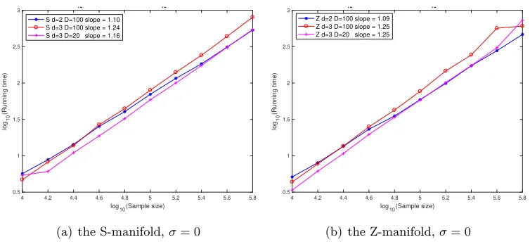
3.1.3. Running time versus sample size n
The complexity of GMRA is O(CdDnlogn). In Figure 7, we display the average running time of GMRA in 10 experiments for the S and Z manifolds when d = 2, D = 100 and d= 3, D= 100 andd= 3, D= 20. The running time of GMRA is almost linear in n. The running time increases as dand D increase since the complexity of GMRA is exponential indand linear inD.
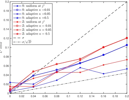
3.1.4. Robustness of GMRA and Adaptive GMRA
The robustness of the empirical GMRA and Adaptive GMRA is tested on the 3-dim S and Z-manifolds embedded inR100 while σ varies butnis fixed to be 105. Figure 8 shows that
the averageL2 approximation error in 10 trails increases linearly with respect toσfor both uniform and Adaptive GMRA with κ∈ {0.01,0.05,0.5}.
3.2. 3D shapes
We run GMRA and Adaptive GMRA on 3D points clouds on the teapot, armadillo and dragon in Figure 9. The teapot data are from the matlab toolbox and others are from the Stanford 3D Scanning Repositoryhttp://graphics.stanford.edu/data/3Dscanrep/.
Figure 9 shows that the adaptive partitions chosen by Adaptive GMRA matches our expectation that, at irregular locations, cells are selected at finer scales than at “flat” locations.
In Figure 10, we display the absolute L2/L∞ approximation error on test data versus
Figure 8: The average L2
approxi-mation error in 10 trails versus σ for GMRA and Adaptive GMRA with κ∈ {0.01,0.05,0.5} on data sampled on the 3-dim S and Z-manifolds. This shows the error of approximation grows linearly with the noise size, suggesting robustness in the construction.
0 0.02 0.04 0.06 0.08 0.1 0.12 0.14 0.16 0.18 0.2 0
0.02 0.04 0.06 0.08 0.1 0.12 0.14 0.16 0.18 0.2
linear, the center approximation is piecewise constant. Both approximation errors decay from coarse to fine scales, but GMRA yields a smaller error than the approximation by local centers. In the middle column, we run GMRA and Adaptive GMRA with theL2 refinement criterion defined in Table 2 with scale-dependent (∆j,k ≥ 2−jτn) and scale-independent
(∆j,k ≥τn) threshold respectively, and display the log-log plot of theL2approximation error
versus the partition size. Overall Adaptive GMRA yields the sameL2 approximation error as GMRA with a smaller partition size, but the difference is insignificant in the armadillo and dragon, as these 3D shapes are complicated and theL2 error simply averages the error at all locations. Then we implement Adaptive GMRA with the L∞ refinement criterion:
b
∆∞j,k = maxxi∈Cj,kkPbj+1xi−Pbjxik and display the log-log plot of the L∞ approximation error versus the partition size in the right column. In theL∞ error, Adaptive GMRA saves a considerable number (about half) of cells in order to achieve the same approximation error as GMRA. In this experiment, scale-independent threshold is slightly better than scale-dependent threshold in terms of saving the partition size.
3.3. MNIST digit data
We consider the MNIST data set fromhttp://yann.lecun.com/exdb/mnist/, which con-tains images of 60,000 handwritten digits, each of size 28×28, grayscale. The intrinsic dimension of this data set varies for different digits and across scales, as it was observed in Little et al. (2017). We run GMRA by setting the diameter of cells at scalej to beO(0.9j) in order to slowly zoom into the data at multiple scales.
We evenly split the digits to the training set and the test set. As the intrinsic dimension is not well-defined, we set GMRA to pick the dimension of Vbj,k adaptively, as the smallest
dimension needed to capture 50% of the energy of the data in Cj,k. As an example, we
display the GMRA approximations of the digit 0,1,2 from coarse scales to fine scales in Figure 11. The histogram of the dimensions of the subspaces Vbj,k is displayed in (a). (b)
represents log10kPbj+1xi−Pbjxikfrom the coarsest scale (top) to the finest scale (bottom),
(a) 41,472 points (b) 165,954 points (c) 437,645 points
(d) κ≈0.18, partition size = 338 (e)κ≈0.41, partition size = 749 (f) κ≈0.63, partition size = 1141
Figure 9: Top line: 3D shapes; bottom line: adaptive partitions selected with refinement criterion∆bj,k ≥2−jκ
p
(logn)/n. Every cell is colored by scale. In the adaptive
partition, at irregular locations cells are selected at finer scales than at “flat” locations.
scale information than the other digits. In (c), we display the log-log plot of the relative L2 error versus scale in GMRA and the center approximation. The improvement of GMRA
over center approximation is noticeable. Then we compute the relativeL2 error for GMRA and Adaptive GMRA when the partition size varies. Figure 11 (d) shows that Adaptive GMRA achieves the same accuracy as GMRA with fewer cells in the partition. Errors increase when the partition size exceeds 103 due to a large variance at fine scales. In this experiment, scale-dependent threshold and scale-independent threshold yield similar performances.
3.4. Natural image patches
It was argued in Peyr´e (2009) that many sets of patches extracted from natural images can be modeled a low-dimensional manifold. We use the Caltech 101 dataset fromhttps:
//www.vision.caltech.edu/Image_Datasets/Caltech101/(see F. Li and Perona, 2006),