An Overview of Independent Component Analysis and Its Applications
Ganesh R. Naik and Dinesh K Kumar
School of Electrical and Computer Engineering RMIT University, Australia
E-mail: [email protected]
Overview paper
Keywords:independent component analysis, blind source separation, non-gaussianity, multi run ICA, overcomplete ICA, undercomplete ICA
Received:July 3, 2009
Independent Component Analysis (ICA), a computationally efficient blind source separation technique, has been an area of interest for researchers for many practical applications in various fields of science and engineering. This paper attempts to cover the fundamental concepts involved in ICA techniques and review its applications. A thorough discussion of the applications and ambiguities problems of ICA has been carried out.Different ICA methods and their applications in various disciplines of science and engineering have been reviewed. In this paper, we present ICA methods from the basics to their potential applications to serve as a comprehensive single source for an inquisitive researcher to carry out research in this field.
Povzetek: Podan je pregled tehnike ICA (Independent Component Analysis).
1
Introduction
The problem of source separation is an inductive inference problem. There is not enough information to deduce the solution, so one must use any available information to in-fer the most probable solution. The aim is to process these observations in such a way that the original source signals are extracted by the adaptive system. The problem of sep-arating and estimating the original source waveforms from the sensor array, without knowing the transmission chan-nel characteristics and the source can be briefly expressed as problems related to BSS. In BSS the word blind refers to the fact that we do not know how the signals were mixed or how they were generated. As such, the separation is in principle impossible. Allowing some relatively indirect and general constrains, we however still hold the term BSS valid, and separate under these conditions.
There appears to be something magical about blind source separation; we are estimating the original source signals without knowing the parameters of mixing and/or filtering processes. It is difficult to imagine that one can estimate this at all. In fact, without some a priori knowl-edge, it is not possible to uniquely estimate the original source signals. However, one can usually estimate them up to certain indeterminacies. In mathematical terms, these indeterminacies and ambiguities can be expressed as arbi-trary scaling, permutation and delay of estimated source signals [1]. These indeterminacies preserve, however, the waveforms of the original sources. Although these inde-terminacies seem to be rather severe limitations, in a great number of applications these limitations are not essential, since the most relevant information about the source signals
is contained in the temporal waveforms or time-frequency patterns of the source signals and usually not in their ampli-tudes or the order in which they are arranged in the output of the system. However, for some applications especially biomedical signal models such as sEMG signals, there is no guarantee that the estimated or extracted signals have exactly the same waveforms as the source signals.
Independent component analysis (ICA) is one of the most widely used BSS techniques for revealing hidden fac-tors that underlie sets of random variables, measurements, or signals. ICA is essentially a method for extracting in-dividual signals from mixtures. Its power resides in the physical assumptions that the different physical processes generate unrelated signals. The simple and generic nature of this assumption allows ICA to be successfully applied in diverse range of research fields.
In this paper, we first set the scene of the blind source separation problem. Then, Independent Component Anal-ysis is introduced as a widely used technique for solving the blind source separation problem. A general description of the approach to achieving separation via ICA and the underlying assumptions of the ICA framework and impor-tant ambiguities that are inherent to ICA are discussed in section 3. A description of specific details of different ICA methods are given in Sections 4, and the paper concludes with applications of BSS and ICA methods.
2
Blind source separation (BSS)
Fa-miliar situations in which this occurs are a crowded room with many people speaking at the same time, interfering electromagnetic waves from mobile phones or crosstalk from brain waves originating from different areas of the brain. In each of these situations the mixed signals are of-ten incomprehensible and it is of interest to separate the individual signals. This is the goal of Blind Source Separa-tion. A classic problem in BSS is the cocktail party prob-lem. The objective is to sample a mixture of spoken voices, with a given number of microphones - the observations, and then separate each voice into a separate speaker channel -the sources. The BSS is unsupervised and thought of as a black box method. In this we encounter many problems, e.g. time delay between microphones, echo, amplitude dif-ference, voice order in speaker and underdetermined mix-ture signal.
Herault and Jutten [2] proposed that, in a artificial neu-ral network like architecture the separation could be done by reducing redundancy between signals. This approach initially lead to what is known as independent component analysis today. The fundamental research involved only a handful of researchers up until 1995. It was not until then, when Bell and Sejnowski [3] published a relatively sim-ple approach to the problem named infomax, that many be-came aware of the potential of ICA. Since then a whole community has evolved around ICA, centralized around some large research groups and its own ongoing confer-ence, International Conference on independent component analysis and blind signal separation. ICA is used today in many different applications, e.g. medical signal analysis, sound separation, image processing, dimension reduction, coding and text analysis [4, 5, 6, 7, 8, 9, 10, 11, 12, 13, 14]. In ICA the general idea is to separate the signals, as-suming that the original underlying source signals are mu-tually independently distributed. Due to the field’s rela-tively young age, the distinction between BSS and ICA is not fully clear. When regarding ICA, the basic frame-work for most researchers has been to assume that the mix-ing is instantaneous and linear, as in infomax. ICA is of-ten described as an exof-tension to PCA, that uncorrelates the signals for higher order moments and produces a non-orthogonal basis. More complex models assume for ex-ample, noisy mixtures, [15, 16], nontrivial source distribu-tions, [17, 18], convolutive mixtures [19, 20, 21], time de-pendency, underdetermined sources [22, 23], mixture and classification of independent component [4, 24]. A general introduction and overview can be found in [25].
3
Independent component analysis
Independent Component Analysis (ICA) is a statistical technique, perhaps the most widely used, for solving the blind source separation problem [25, 26]. In this sec-tion, we present the basic Independent Component Analy-sis model and show under which conditions its parameters can be estimated.
3.1
ICA model
The general model for ICA is that the sources are gener-ated through a linear basis transformation, where additive noise can be present. Suppose we haveN statistically in-dependent signals, si(t),i=1, ...,N. We assume that the
sources themselves cannot be directly observed and that each signal,si(t), is a realization of some fixed probability
distribution at each time pointt. Also, suppose we observe these signals usingNsensors, then we obtain a set ofN ob-servation signalsxi(t),i=1, ...,N that are mixtures of the
sources. A fundamental aspect of the mixing process is that the sensors must be spatially separated (e.g. microphones that are spatially distributed around a room) so that each sensor records a different mixture of the sources. With this spatial separation assumption in mind, we can model the mixing process with matrix multiplication as follows:
x(t) =As(t) (1)
whereAis an unknown matrix called themixing matrix
andx(t),s(t) are the two vectors representing the observed signals and source signals respectively. Incidentally, the justification for the description of this signal processing technique asblind is that we have no information on the mixing matrix, or even on the sources themselves.
The objective is to recover the original signals, si(t),
from only the observed vectorxi(t). We obtain estimates
for the sources by first obtaining the “unmixing matrix”W, where,W=A−1.
This enables an estimate, ˆs(t), of the independent sources to be obtained:
ˆ
s(t) =W x(t) (2)
The diagram in Figure 1 illustrates both the mixing and unmixing process involved in BSS. The independent sources are mixed by the matrixA(which is unknown in this case). We seek to obtain a vector y that approximates s by estimating the unmixing matrixW. If the estimate of the unmixing matrix is accurate, we obtain a good approx-imation of the sources.
The above described ICA model is the simple model since it ignores all noise components and any time delay in the recordings.
3.2
Independence
A key concept that constitutes the foundation of indepen-dent component analysis is statistical independence. To simplify the above discussion consider the case of two dif-ferent random variabless1ands2. The random variables1
is independent ofs2, if the information about the value of
s1does not provide any information about the value ofs2,
and vice versa. Here s1 ands2 could be random signals
Figure 1: Blind source separation (BSS) block diagram.s(t)are the sources.x(t)are the recordings, ˆs(t)are the estimated sourcesAis mixing matrix andW is un-mixing matrix
3.2.1 Independence definition
Mathematically, statistical independence is defined in terms of probability density of the signals. Consider the joint probability density function (pdf) of s1 and s2 be
p(s1,s2). Let the marginal pdf ofs1ands2be denoted by
p1(s1)andp2(s2)respectively. s1ands2are said to be
in-dependent if and only if the joint pdf can be expressed as;
ps1,s2(s1,s2) =p1(s1)p2(s2) (3) Similarly, independence could be defined by replacing the pdf by the respective cumulative distributive functions as;
E{p(s1)p(s2)}=E{g1(s1)}E{g2(s2)} (4)
where E{.} is the expectation operator. In the following section we use the above properties to explain the relation-ship between uncorrelated and independence.
3.2.2 Uncorrelatedness and Independence
Two random variabless1ands2are said to be uncorrelated
if their covarianceC(s1,s1) is zero.
C(s1,s2) =E{(s1−ms1)(s2−ms2)}
=E{s1s2−s1ms2−s2ms1+ms1ms2}
=E{s1s2} −E{s1}E{s2}
=0
(5)
wherems1is the mean of the signal. Equation 4 and 5
are identical for independent variables takingg1(s1) =s1.
Hence independent variables are always uncorrelated. How ever the opposite is not always true. The above discussion proves that independence is stronger than uncorrelatedness and hence independence is used as the basic principle for ICA source estimation process. However uncorrelatedness is also important for computing the mixing matrix in ICA.
3.2.3 Non-Gaussianity and Independence
According to central limit theorem the distribution of a sum of independent signals with arbitrary distributions tends to-ward a Gaussian distribution under certain conditions. The sum of two independent signals usually has a distribution that is closer to Gaussian than distribution of the two orig-inal signals. Thus a gaussian signal can be considered as a liner combination of many independent signals. This fur-thermore elucidate that separation of independent signals from their mixtures can be accomplished by making the linear signal transformation as non-Gaussian as possible.
Non-Gaussianity is an important and essential principle in ICA estimation. To use non-Gaussianity in ICA es-timation, there needs to be quantitative measure of Gaussianity of a signal. Before using any measures of non-Gaussianity, the signals should be normalised. Some of the commonly used measures are kurtosis and entropy mea-sures, which are explained next.
– Kurtosis
Kurtosis is the classical method of measuring Non-Gaussianity. When data is preprocessed to have unit vari-ance, kurtosis is equal to the fourth moment of the data.
The Kurtosis of signal (s), denoted bykurt(s), is defined by
kurt(s) =E{s4} −3(E{s4})2 (6) This is a basic definition of kurtosis using higher or-der (fourth oror-der) cumulant, this simplification is based on the assumption that the signal has zero mean. To simplify things, we can further assume that (s) has been normalised so that its variance is equal to one:E{s2}=1.
Hence equation 6 can be further simplified to
E{s4}=3(E{s4})2 and hence its kurtosis is zero. For most non-Gaussian signals, the kurtosis is nonzero. Kur-tosis can be both positive or negative. Random variables that have positive kurtosis are called assuper Gaussian or
platykurtotic, and those with negative kurtosis are called assub Gaussianorleptokurtotic. Non-Gaussianity is mea-sured using the absolute value of kurtosis or the square of kurtosis.
Kurtosis has been widely used as measure of Non-Gaussianity in ICA and related fields because of its com-putational and theoretical and simplicity. Theoretically, it has a linearity property such that
kurt(s1±s2) =kurt(s1)±kurt(s2) (8)
and
kurt(αs1) =α4kurt(s1) (9)
whereα is a constant. Computationally kurtosis can be calculated using the fourth moment of the sample data, by keeping the variance of the signal constant.
In an intuitive sense, kurtosis measured how "spikiness" of a distribution or the size of the tails. Kurtosis is ex-tremely simple to calculate, however, it is very sensitive to outliers in the data set. It values may be based on only a few values in the tails which means that its statistical sig-nificance is poor. Kurtosis is not robust enough for ICA. Hence a better measure of non-Gaussianity than kurtosis is required.
– Entropy
Entropy is a measure of the uniformity of the distribution of a bounded set of values, such that a complete unifor-mity corresponds to maximum entropy. From the informa-tion theory concept, entropy is considered as the measure of randomness of a signal. Entropy H of discrete-valued signalSis defined as
H(S) =−
∑
P(S=ai)logP(S=ai) (10)This definition of entropy can be generalised for a continuous-valued signal (s), called differential entropy, and is defined as
H(S) =− ∫
p(s)logp(s)ds (11)
One fundamental result of information theory is that Gaussian signal has the largest entropy among the other signal distributions of unit variance. entropy will be small for signals that have distribution concerned on certain val-ues or have pdf that is very "spiky". Hence, entropy can be used as a measure of non-Gaussianity.
In ICA estimation, it is often desired to have a measure of non-Gaussianity which is zero for Gaussian signal and nonzero for non-Gaussian signal for computational sim-plicity. Entropy is closely related to the code length of the random vector. A normalised version of entropy is given by a new measure called NegentropyJwhich is defined as
J(S) =H(sgauss)−H(s) (12)
wheresgauss is the Gaussian signal of the same
covari-ance matrix as (s). Equation 12 shows that Negentropy is always positive and is zero only if the signal is a pure gaus-sian signal. It is stable but difficult to calculate. Hence approximation must be used to estimate entropy values.
3.3
Mathematical Independence
Mathematical properties of matrices were investigated to check the linear dependency and independency of global matrices (Permutation matrixP)
3.3.1 Rank of the matrix
Rank of the matrix will be less than the matrix size for lin-ear dependency and rank will be size of matrix for linlin-ear independency, but this couldn’t be assured yet due to noise in the signal. Hence determinant is the key factor for esti-mating number of sources.
3.3.2 Determinant of the matrix
In real time applications Determinant value should be zero for linear independency and should be more than zero (close to 1) for linear independency [27].
3.4
ICA Assumptions and Ambiguities
ICA is distinguished from other approaches to source sep-aration in that it requires relatively few assumptions on the sources and on the mixing process. The assumptions and of the signal properties and other conditions and the issues related to ambiguities are discussed below:
3.4.1 ICA Assumptions
– The sources being considered are statistically inde-pendent
The first assumption is fundamental to ICA. As dis-cussed in Section 3.2, statistical independence is the key feature that enables estimation of the independent compo-nents ˆs(t)from the observationsxi(t).
– The independent components have non-Gaussian dis-tribution
– The mixing matrix is invertible
The third assumption is straightforward. If the mixing ma-trix is not invertible then clearly the unmixing mama-trix we seek to estimate does not even exist.
If these three assumptions are satisfied, then it is possi-ble to estimate the independent components modulo some trivial ambiguities (discussed in Section 3.4). It is clear that these assumptions are not particularly restrictive and as a result we need only very little information about the mixing process and about the sources themselves.
3.4.2 ICA Ambiguity
There are two inherent ambiguities in the ICA framework. These are (i) magnitude and scaling ambiguity and (ii) per-mutation ambiguity.
– Magnitude and scaling ambiguity
The true variance of the independent components cannot be determined. To explain, we can rewrite the mixing in equation 1 in the form
x=As
=
N
∑
j=1
ajsj
(13)
whereajdenotes the jth column of the mixing matrixA.
Since both the coefficientsajof the mixing matrix and the
independent componentssjare unknown, we can transform
Equation 13.
x=
N
∑
j=1
(1/αjaj)(αjsj) (14)
Fortunately, in most of the applications this ambiguity is insignificant. The natural solution for this is to use as-sumption that each source has unit variance: E{sj2}= 1. Furthermore, the signs of the of the sources cannot be de-termined too. This is generally not a serious problem be-cause the sources can be multiplied by -1 without affecting the model and the estimation
– Permutation ambiguity
The order of the estimated independent components is unspecified. Formally, introducing a permutation matrix P and its inverse into the mixing process in Equation 1.
x=AP−1Ps
=A′s′ (15)
Here the elements of P s are the original sources, ex-cept in a different order, and A′ =AP−1 is another un-known mixing matrix. Equation 15 is indistinguishable from Equation 1 within the ICA framework, demonstrating
that the permutation ambiguity is inherent to Blind Source Separation. This ambiguity is to be expected ˝U in separat-ing the sources we do not seek to impose any restrictions on the order of the separated signals. Thus all permutations of the sources are equally valid.
3.5
Preprocessing
Before examining specific ICA algorithms, it is instructive to discuss preprocessing steps that are generally carried out before ICA.
3.5.1 Centering
A simple preprocessing step that is commonly performed is to “center” the observation vector x by subtracting its mean vectorm=E{x}. That is then we obtain the centered observation vector,xc, as follows:
xc=x−m (16)
This step simplifies ICA algorithms by allowing us to assume a zero mean. Once the unmixing matrix has been estimated using the centered data, we can obtain the actual estimates of the independent components as follows:
ˆ
s(t) =A−1(xc+m) (17)
From this point on, all observation vectors will be as-sumed centered. The mixing matrix, on the other hand, remains the same after this preprocessing, so we can al-ways do this without affecting the estimation of the mixing matrix.
3.5.2 Whitening
Another step which is very useful in practice is to pre-whiten the observation vector x. Whitening involves lin-early transforming the observation vector such that its com-ponents are uncorrelated and have unit variance [27]. Let
xwdenote the whitened vector, then it satisfies the
follow-ing equation:
E{xwxTw}=I (18)
whereE{xwxTw} is the covariance matrix ofxw. Also,
since the ICA framework is insensitive to the variances of the independent components, we can assume without loss of generality that the source vector, s, is white, i.e.
E{ssT}=I
A simple method to perform the whitening transforma-tion is to use the eigenvalue decompositransforma-tion (EVD) [27] of
x. That is, we decompose the covariance matrix ofx as follows:
E{xxT}=V DVT (19)
diag{λ1,λ2, ...,λn}. The observation vector can be
whitened by the following transformation:
xw=V D−1/2VTx (20)
where the matrix D−1/2 is obtained by a simple component wise operation as D−1/2 = diag{λ1−1/2,λ2−1/2, ...,λn−1/2}. Whitening transforms
the mixing matrix into a new one, which is orthogonal
xw=V D−1/2VTAs=Aws (21)
hence,
E{xwxTw}=AwE{ssT}ATw
=AwATw
=I
(22)
Whitening thus reduces the number of parameters to be estimated. Instead of having to estimate then2elements of the original matrixA, we only need to estimate the new or-thogonal mixing matrix, where An oror-thogonal matrix has
n(n−1)/2 degrees of freedom. One can say that whitening solves half of the ICA problem. This is a very useful step as whitening is a simple and efficient process that signifi-cantly reduces the computational complexity of ICA. An il-lustration of the whitening process with simple ICA source separation process is explained in the later section.
3.6
Simple Illustrations of ICA
To clarify the concepts discussed in the preceding sections two simple illustrations of ICA are presented here. The results presented below were obtained using the FastICA algorithm, but could equally well have been obtained from any of the numerous ICA algorithms that have been pub-lished in the literature (including the Bell and Sejnowsiki algorithm).
3.6.1 Separation of Two Signals
This section explains the simple ICA source separation pro-cess. In this illustration two independent signals,s1ands2,
0 200 400 600 800 1000
−1 −0.5 0 0.5 1
0 200 400 600 800 1000
−1 −0.5 0 0.5 1
Original source “ s2 ” Original source “ s1 ”
Figure 2: Independent sourcess1 ands2
0 200 400 600 800 1000
−2 −1 0 1 2
Mixed signal “ x1 ”
Mixed signal “ x2 ”
0 200 400 600 800 1000
−2 −1 0 1 2
Figure 3: Observed signals, x1 andx2, from an unknown linear mixture of unknown independent components
0 200 400 600 800 1000
−2 −1 0 1 2
0 200 400 600 800 1000
−2 −1 0 1 2
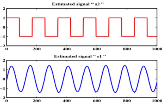
Estimated signal “ s1 ” Estimated signal “ s2 ”
Figure 4: Estimates of independent components
are generated. These signals are shown in Figure2. The in-dependent components are then mixed according to equa-tion 1 using an arbitrarily chosen mixing matrix A, where
A= (
0.3816 0.8678 0.8534 −0.5853
)
The resulting signals from this mixing are shown in Fig-ure 3. Finally, the mixtFig-uresx1andx2are separated using
ICA to obtains1ands2, shown in Figure 4. By comparing
Figure 4 to Figure 2 it is clear that the independent compo-nents have been estimated accurately and that the indepen-dent components have been estimated without any knowl-edge of the components themselves or the mixing process. This example also provides a clear illustration of the scaling and permutation ambiguities discussed in Section 3.4. The amplitudes of the corresponding waveforms in Figures 2 and 4 are different. Thus the estimates of the in-dependent components are some multiple of the indepen-dent components of Figure 3, and in the case of s1, the scaling factor is negative. The permutation ambiguity is also demonstrated as the order of the independent compo-nents has been reversed between Figure 2 and Figure 4.
3.6.2 Illustration of Statistical Independence in ICA
−2 −1.5 −1 −0.5 0 0.5 1 1.5 2 −2
−1.5 −1 −0.5 0 0.5 1 1.5 2
s1 s2
Figure 5: Original sources
−4 −3 −2 −1 0 1 2 3 4
−2 −1.5 −1 −0.5 0 0.5 1 1.5 2
x1
x2
Figure 6: Mixed sources
separate them. However, this gives no insight into the me-chanics of ICA and the close link with statistical indepen-dence. We assume that the independent components can be modeled as realizations of some underlying statistical distribution at each time instant (e.g. a speech signal can be accurately modeled as having a Laplacian distribution). One way of visualizing ICA is that it estimates the optimal linear transform to maximise the independence of the joint distribution of the signalsXi.
The statistical basis of ICA is illustrated more clearly in this example. Consider two random signals which are mixed using the following mixing process:
( x1
x2
) =
(
1 2 1 1
)( s1
s2
)
Figure 5 shows the scatter-plot for original sources s1
ands2. Figure 6 shows the scatter-plot of the mixtures. The
−4 −3 −2 −1 0 1 2 3 4
−4 −3 −2 −1 0 1 2 3 4
x1 x2
Figure 7: Joint density of whitened signals obtained from whitening the mixed sources
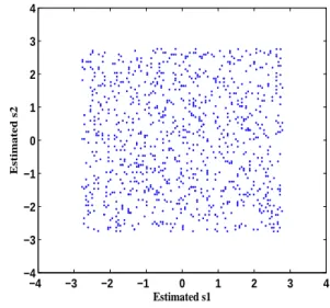
−4 −3 −2 −1 0 1 2 3 4
−4 −3 −2 −1 0 1 2 3 4
Estimated s1
Estimated s2
Figure 8: ICA solution (Estimated sources)
distribution along the axisx1andx2are now dependent and
the form of the density is stretched according to the mixing matrix. From the Figure 6 it is clear that the two signals are not statistically independent because, for example, ifx1=
-3 or 3 thenx2is totally determined. Whitening is an
inter-mediate step before ICA is applied. The joint distribution that results from whitening the signals of Figure 6 is shown in Figure 7. By applying ICA, we seek to transform the data such that we obtain two independent components.
The joint distribution resulting from applying ICA to
x1 andx2 is shown in Figure 7. This is clearly the joint
distribution of two independent, uniformly distributed ran-dom variables. Independence can be intuitively confirmed as each random variable is unconstrained regardless of the value of the other random variable (this is not the case for
Figure 8 take values between 3 and -3, but due to the scal-ing ambiguity, we do not know the range of the original independent components. By comparing the whitened data of Figure 7 with Figure 8, we can see that, in this case, pre-whitening reduces ICA to finding an appropriate rotation to yield independence. This is a simplification as a rotation is an orthogonal transformation which requires only one pa-rameter.
The two examples in this section are simple but they il-lustrate both how ICA is used and the statistical underpin-nings of the process. The power of ICA is that an identical approach can be used to address problems of much greater complexity.
3.7
ICA Algorithms
There are several ICA algorithms available in literature. How ever the following three algorithms are widely used in numerous signal processing applications. These includes FastICA, JADE, and Infomax. Each algorithm used a dif-ferent approach to solve equation.
3.7.1 FastICA
FastICA is a fixed point ICA algorithm that employs higher order statistics for the recovery of independent sources. FastICA can estimate ICs one by one (deflation approach) or simultaneously (symmetric approach). FastICA uses simple estimates of Negentropy based on the maximum en-tropy principle, which requires the use of appropriate non-linearities for the learning rule of the neural network.
Fixed point algorithm is based on the mutual informa-tion. Which can be written as:
I(s) = ∫
fs(s)log
fs(s)
∏fsi(si)
ds (23)
This measure is kind of distance of independence. Min-imising mutual information leads to ICA solution. For the fast ICA algorithm the above equation is re written as
I(s) =J(s)−
∑
i
Jsi+
1 2log
∏Cii
detCss
(24)
where ˆs=W x,Css is the correlation matrix, andcii is
theith diagonal element of the correlation matrix. The last term is zero because si are supposed to be uncorrelated.
The first term is constant for a problem, because of the in-variance in Negentropy. The problem is now reduced to separately maximising the Negentropy of each component. Estimation of Negentropy is a delicate problem. The pa-pers [28][ [1] and [2] [29]
have addressed this problem. For the general version of fixed point algorithm, the approximation was based on a maximum entropy principle. The algorithm works with whitened data, although aversion of non-whitened data ex-ists.
– Criteria
The maximisation is preferred over the following index
JG(w) = [E{G(wTv)} −E{G(ν)}2 (25)
to find one independent component, withνstandard gaus-sian variable, andG, the one unit contrast function.
– Update rule
Update rule for the generic algorithm is
w∗=E{vg(wTv)} −E{g′(wTv)}w
w=w∗/∥w∗∥ (26)
to extract one component. There is symmetric version of the FP algorithm, whose update rule is
W∗=E{g(W v)vT} −Diag(E{g′(W v)})W W= (W∗W∗T)−1/2W∗
(27)
whereDiag(v)is a diagonal matrix withDiagii(v) =vi.
– Parameters
FastICA uses the following nonlinear parameters for convergence.
g(y) = {
y3
tanh(y) (28)
The choice is free except that the symmetric algorithm with tanh non linearity does not separate super Gaus-sian signals. Otherwise the choice can be devoted to the other criteria, for instance the cubic non linearity is faster, whereas thetanhlinearity is more stable. These questions are addressed in [25]
In practice, the expectations in FastICA must be replaced by their estimates. The natural estimates are of course the corresponding sample means. Ideally, all the data available should be used, but this is often not a good idea because the computations may become too demanding. Then the aver-ages can be estimated using a smaller sample, whose size may have a considerable effect on the accuracy of the final estimates. The sample points should be chosen separately at every iteration. If the convergence is not satisfactory, one may then increase the sample size. This thesis uses FastICA algorithm for all applications.
3.7.2 Infomax
The algorithm is derived through an information max-imisation principle, applied here between the inputs and the non linear outputs. Given the form of joint entropy
H(s1,s2) =H(s1) +H(s2)−I(s1,s2) (29)
Here for two variabless=g(Bx), it is clear that maximis-ing the joint entropy of the outputs amounts to minimismaximis-ing mutual informationI(y1,y2), unless it is more interesting to
maximise the individual entropies than to reduce the mu-tual information. This is the point, where the nonlinear function plays an important role.
The basic idea of the information maximisation is to match the slope of the nonlinear function with the input probability density function. That is
s=g(x,θ)≃ ∫ x
−inf
fx(t)dt (30)
In case of perfect matching fs(s)looks like an uniform
variable, whose entropy is large. If this is not possible be-cause the shapes are different, the best solution found in some case is to mix the input distributions so that the re-sulting mix matches the slope of the transfer function better than a single input distribution. In this case the algorithm does not converge, and the separation is not achieved.
– Criteria
The algorithm is a stochastic gradient ascent that max-imises the joint entropy (Eqn. 12).
– Update rule
In its original form, the update rule is
∆B=λ[[BT]−1+ (1−2g(Bx+b0))xT]
∆b=λ[1−2g(Bx+b0)]
(31)
– Parameters
The nonlinear function used in the original algorithm is
g(s) = 1
1+e−s (32)
and in the extended version, it is
g(s) =s±tanh(s) (33)
where the sign is that of the estimated kurtosis of the signal.
The information maximization algorithm (often referred as infomax) is widely used to separate super-Gaussian sources. Infomax is a gradient-based neural network algo-rithm, with a learning rule for information maximization. Infomax uses higher order statistics for the information maximization. The information maximization is attained by maximizing the joint entropy of a transformed vector.
z=g(W x), whereg is a point wise sigmoidal nonlinear function.
4
ICA for different conditions
One of the important conditions of ICA is that the num-ber of sensors should be equal to the numnum-ber of sources. Unfortunately, the real source separation problem does not always satisfy this constraint. This section focusses on ICA source separation problem under different conditions where the number of sources are not equal to the number of recordings.
4.1
Overcomplete ICA
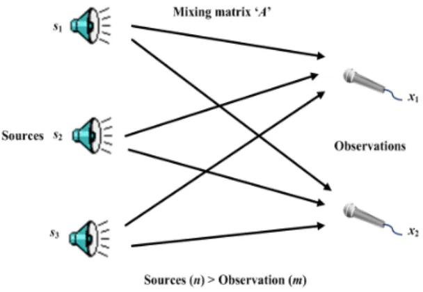
Overcomplete ICA is one of the ICA source separation problem where the number of sources are greater than the number of sensors, i.e (n>m). The ideas used for over-complete ICA originally stem from coding theory, where the task is to find a representation of some signals in a given set of generators which often are more numerous than the signals, hence the term overcomplete basis. Sometimes this representation is advantageous as it uses as few ‘basis’ ele-ments as possible, referred to as sparse coding. Olshausen and Field [30] first put these ideas into an information the-oretic context by decomposing natural images into an over-complete basis. Later, Harpur and Prager [31] and, inde-pendently, Olshausen [32] presented a connection between sparse coding and ICA in the square case. Lewicki and Sejnowski [22] then were the first to apply these terms to overcomplete ICA, which was further studied and applied by Lee et al. [33]. De Lathauwer et al. [34] provided an interesting algebraic approach to overcomplete ICA of three sources and two mixtures by solving a system of lin-ear equations in the third and fourth-order cumulants, and Bofill and Zibulevsky [35] treated a special case (‘delta-like’ source distributions) of source signals after Fourier transformation. Overcomplete ICA has major applications in bio signal processing, due to the limited number of elec-trodes (recordings) compared to the number active muscles (sources) involved (in certain cases unlimited).
Figure 9: Illustration of “overcomplete ICA"
In overcomplete ICA, the number of sources exceed number of recordings. To analyse this, consider two recordingsx1(t)andx2(t)from three independent sources
of thesi(t), where the coefficients depend on the distances
between the sources and the sensors (refer Figure 9):
x1(t) =a11s1(t) +a12s2(t) +a13s3(t) (34)
x2(t) =a21s1(t) +a22s2(t) +a23s3(t)
The ai j are constant coefficients that give the mixing
weights. The mixing process of these vectors can be repre-sented in the matrix form as (refer Equation 1):
( x1
x2
) =
(
a11 a12 a13
a21 a22 a23
) ss12
s3
The unmixing process and estimation of sources can be written as (refer Equation 2):
ss12
s3
=
ww1121 ww1222
w31 w32
(x1
x2
)
In this example matrixAof size 2×3 matrix and unmix-ing matrixW is of size 3×2. Hence in overcomplete ICA it always results in pseudoinverse. Hence computation of sources in overcomplete ICA requires some estimation pro-cesses.
4.1.1 Overcomplete ICA methods
There are two common approaches of solving the overcom-plete problem.
– Single step approach where the mixing matrix and the independent sources are estimated at once in a single algorithm
– Two step algorithm where the mixing matrix and the independent component values are estimated with dif-ferent algorithms.
Lewicki and Sejnowski [22] proposed the single step ap-proach, which is a natural solution to decomposition by finding the maximum a posteriori representation of the data. The prior distribution on the basis function coeffi-cients removes the redundancy in the representation and leads to representations that are sparse and are nonlinear functions of the data. The probabilistic approach to de-composition also leads to a natural method of denoising. From this model, they derived a simple and robust learning algorithm by maximizing the data likelihood over the basis functions. Another approach in single step was proposed by Shriki et al. [36] using recurrent model, i.e., the es-timated independent sources are computed taking into ac-count the influence of other independent sources.
One of the disadvantage of single step approach is that it is complex and computationally expensive. Hence many researchers have proposed the two step method, where the mixing matrix is estimated in the first step and the sources are recovered in the next step. Zibulevsky et al. [35] pro-posed a sparse overcomplete ICA with delta distributions.
Fabian Theis [37, 38] proposed geometric overcomplete ICA. Recently Waheed et. al [39, 40] demonstrated alge-braic overcomplete ICA. In this thesis Zibulevsky’s sparse overcomplete ICA is utilised, which is explained in the next section.
4.1.2 Sparse overcomplete ICA
Sparse representation of signals which is modeled by ma-trix factorisation has been receiving a great deal of inter-est in recent years. The research community has invinter-esti- investi-gated many linear transforms that make audio, video and image data sparse, such as the Discrete Cosine Transform (DCT), the Fourier transform, the wavelet transform and their derivatives. [41]. Chen et al. [42] discussed sparse representations of signals by using large scale linear pro-gramming under given overcomplete basis (e.g., wavelets). Olshausen et al. [43] represented sparse coding of im-ages based on maximum posterior approach but it was Zibulevsky et al. [35] who noticed that in the case of sparse sources, their linear mixtures can be easily separated us-ing very simple “geometric" algorithms. Sparse represen-tations can be used in blind source separation. When the sources are sparse, smaller coefficients are more likely and thus for a given data pointt, if one of the sources is sig-nificantly larger, the remaining ones are likely to be close to zero. Thus the density of data in the mixture space, be-sides decreasing with the distance from the origin shows a clear tendency to cluster along the directions of the basis vectors. Sparsity is good in ICA for two reasons. First the statistical accuracy with which the mixing matrixAcan be estimated is a function of how non-Gaussian the source dis-tributions are. This suggests that the sparser the sources are the less data is needed to estimateA. Secondly the quality of the source estimates givenA, is also better for sparser sources. A signal is considered sparse when values of most of the samples of the signal do not differ significantly from zero. These are from sources that are minimally active. Zibulevsky et al. [35] have demonstrated that when the signals are sparse, and the sources of these are indepen-dent, these may be separated even when the number of sources exceeds the number of recordings. [35]. The over-complete limitation suffered by normal ICA is no longer a limiting factor for signals that are very sparse. Zibulevsky also demonstrated that when the signals are sparse, it is possible to determine the number of independent sources in a mixture of unknown signal numbers.
– Source estimation
x=As+ξ (35) whereξ represents noise in the recordings. It is assumed that the independent sourcesscan be sparsely represented in a proper signal dictionary
si= K
∑
k=1
Ckiφk (36)
whereφk are theatomsorelementsof the dictionary.
Im-portant examples are wavelet-related dictionaries such as wavelet and wavelet packets [41]. Equation 36 can be ex-pressed in matrix notation as
s=CΦ (37)
by substituting Equation 37 into 35 gives
x=ACΦ+ξ (38)
The goal is to estimate the mixing matrixAand the coef-ficientsCat the same time so thatCis as sparse as possible. andX≈ACΦ, given only the observed dataxand the dic-tionaryΦ
Using maximum a posteriori approach, the above goal can be expressed as
max
A,C P(A,C|x)∝maxA,CP(x|A,C)P(A)P(C) (39)
Taking into account Equation 35 and Gaussian noise, the conditional probabilityP(x|A,C)can be expressed as
P(x|A,C)∝
∏
i
exp[−(xi−(ACΦ)i)
2
2σ2 ] (40)
SinceC is assumed to be sparse, it can be approximated with the following pdf
pi(Cki)∝exp[−(βih(Cik))] (41)
and hence
p(C)∝
∏
i,k
exp[−(βih(Cik))] (42)
Assuming the pdf ofP(A)to be uniform, Equation 39 can now be simplified as
max
A,C P(A,C|x)∝maxA,CP(x|A,C)P(C) (43)
Finally, the optimisation problem can be formed by substi-tuting 40 and 42 into 43, taking the logarithm and inverting the sign
max
A,C P(A,C|x)∝minA,C
1
2σ2|ACΦ−x∥ 2
F+
∑
i,k
(βih(Cik))
(44)
There are several measures of sparsity. The simplest measure is thel0norm. One of the drawback of this
mea-sure is that, it is discontinuous and difficult to optimise, and also very sensitive to noise. The closest approximation of
l0 isl1norm. The validity of this measure can be shown
by simplifying equation 44 under zero noise assumption and under Laplacian prior distributions withh(Ck
i) =|Cki|.
Under these assumptions the optimisation problem can be decomposed intoKsmaller problems for each data pointck
at time point
k=1...Kas
min
ck
∑
i
|cki| (45)
subject to Ackφk=xk. If small signalsis sparse in time
domain thenckin equation 45 can be uploaded withsk.
min
sk
∑
i
|ski| (46)
subject toAsk=xk. Equation 46 can be formulated as linear programming in basic form as
min
sk c
Tsk| (47)
subject toAsk=xk,sk≥0 wheresk⇔[uk;vk],A⇔[A;−A]
andc⇔[1; 1].
– Estimating the mixing matrix
The second step in two step approach is estimating the mixing matrix. There exists various methods to compute the mixing matrix in sparse overcomplete ICA. The most widely used techniques are:
(i) C-means clustering (ii) Algebraic method and
(iii) Potential function based method
All the above mentioned methods are based on the clus-tering principle. The difference is the way they estimate the direction of the clusters. The sparsity of the signal plays an important role for estimating the mixing matrix. A simple illustration that is useful to understand this concept can be found in
4.2
Undercomplete ICA
number of principal recordings as the number of sources discarding the rest. To analyse this, consider three record-ings x1(t),x2(t)andx3(t)from two independent sources
s1(t)ands2(t). Thexi(t)are then weighted sums of the
si(t), where the coefficients depend on the distances
be-tween the sources and the sensors (refer Figure 10):
Figure 10: Illustration of “undercomplete ICA"
x1(t) =a11s1(t) +a12s2(t)
x2(t) =a21s1(t) +a22s2(t) (48)
x3(t) =a31s1(t) +a32s2(t)
The ai j are constant coefficients that gives the mixing
weights. The mixing process of these vectors can be repre-sented in the matrix form as:
xx12
x3
=
aa1121 aa1222
a31 a32
(s1
s2
)
The unmixing process using the standard ICA requires a di-mensional reduction approach so that, if one of the record-ings is reduced then the square mixing matrix is obtained, which can use any standard ICA for the source estimation. For instance one of the recordings sayx3is redundant then
the above mixing process can be written as:
( x1
x2
) =
(
a11 a12
a21 a22
)( s1
s2
)
Hence unmixing process can use any standard ICA algo-rithm using the following:
( s1
s2
) =
(
w11 w12
w21 w22
)( x1
x2
)
The above process illustrates that, prior to source signal separation using undercomplete ICA, it is important to re-duce the dimensionality of the mixing matrix and identify the required and discard the redundant recordings. Princi-pal Component Analysis (PCA) is one of the powerful di-mensional reduction method used in signal processing ap-plications, which is explained next.
4.2.1 Undercomplete ICA using dimensional reduction method
When the number of recordingsnare more than the num-ber of sourcesm, there must be information redundancy in the recordings. Hence the first step is to reduce the dimen-sionality of the recorded data. If the dimendimen-sionality of the recorded data is equal to that of the sources, then standard ICA methods can be applied to estimate the independent sources. An example of this stages methods is illustrated in [44].
One of the popular method used in dimensional reduc-tion method is PCA. PCA uses the decorrelated method to reduce the recorded dataxusing a matrixV
z=V x (49)
such thatEzzT =I. The transformation matrixV is given by
V=D12ET (50)
whereDandEare the Eigenvalue and Eigenvector decom-position of covariance matrixCx
Cx=ED
1
2ET (51)
Now it can be proven that
E{zzT}=V E{xxT}VT
=D−1/2ETEDETED−1/2 =I
(52)
The second stage is using any of the standard ICA al-gorithms discussed in Section 3.2 to estimate the sources. In fact, whitening process through PCA is standard prepro-cessing in ICA. It means that applying any standard ICA al-gorithms that incorporates PCA will automatically reduce the dimension before running ICA.
4.3
Sub band decomposition ICA
Figure 11: Sub band ICA block diagram.
Such wide-band source signals are a linear decomposi-tion of several narrow-band sub components (refer Figure 11):
s(t) =s1(t) +s2(t) +s3(t), . . . ,sn(t) (53)
Such decomposition can be modeled in the time, fre-quency or time frefre-quency domains using any suitable lin-ear transform. A set of unmixing or separating matrices:
W1,W2,W3,. . . ,Wn are obtained whereW1 is the unmixing
matrix for sensor datax1(t)andWnis the unmixing matrix
for sensor dataxn(t). If the specific sub-components of
in-terest are mutually independent for at least two sub-bands, or more generally two subsets of multi-band, say for the sub band “p" and sub band “q" then the global matrix
Gpq=Wp×Wq−1 (54)
will be a sparse generalized permutation matrixPwith spe-cial structure with only one non-zero (or strongly dominat-ing) element in each row and each column [27]. This fol-lows from the simple mathematical observation that in such case both matricesWpandWqrepresent pseudo-inverses (or
true inverse in the case of square matrix) of the same true mixing matrixA (ignoring non-essential and unavoidable arbitrary scaling and permutation of the columns) and by making an assumption that sources for two multi-frequency sub-bands are independent. This provides the basis for sep-aration of dependent sources using narrow band pass fil-tered sub band signals for ICA.
4.4
Multi run ICA
One of the most effective ways of modeling vector data for unsupervised pattern classification or coding is to assume that the observations are the result of randomly picking out of a fixed set of different distributions. ICA is an iterative BSS technique. At each instance original signals are es-timated from the mixed data. The quality of estimation of the original signals depends mainly on the unmixing matrix
W. Due to the randomness associated with the estimation
of the unmixing matrix and the iterative process, there is a randomness associated with the quality of separation.
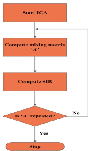
Figure 12: Multi run ICA mixing matrix computation flow chart
Multi run ICA has been proposed to overcome this asso-ciated randomness. [45]. It is the process where the ICA algorithm will be computed many times; at each instance different mixing matrices will be estimated. A1,A2, ...,An.
Since it is an iterative technique with inbuilt quantisation, repeat analysis yields similarity matrices at some stage. Hence mixing matricesA1,A2etc, will repeat after certain
iterations. To estimate the sources from the mixed data ICA requires just one mixing matrix, the best unmixing matrix would give clear source separation, hence the selection of the best matrix is the key criterion in multi run ICA. There exists several methods to compute the quality of the mixing matrices, they are
– Signal to Noise Ratio (SNR) – Signal to Interference Ratio (SIR) – Signal to Distortion Ratio (SDR) and – Signal to Artefacts Ratio (SAR)
best unmixing matrix is estimated, then any normal ICA method can be used for source separation. The multi run ICA computational process flow chart is shown in Figure 12.
5
Applications of ICA
The success of ICA in source separation has resulted in a number of practical applications. These includes,
– Machine fault detection [46, 47, 48, 49] – Seismic monitoring [50, 51]
– Reflection canceling [52, 53]
– Finding hidden factors in financial data [54, 55, 56] – Text document analysis [4, 5, 6]
– Radio communications [57, 58] – Audio signal processing [20, 13]
– Image processing [13, 14, 59, 60, 61, 62, 63] – Data mining [64]
– Time series forecasting [65]
– Defect detection in patterned display surfaces [66,?] – Bio medical signal processing [7, 67, 8, 9, 10, 11, 12,
68, 69].
Some of the major applications are explained in detail next:
5.1
Biomedical Applications of ICA
Exemplary ICA applications in biomedical problems in-clude the following:
– Fetal Electrocardiogram extraction, i.e removing/fil-tering maternal electrocardiogram signals and noise from fetal electrocardiogram signals [70, 71]. – Enhancement of low level Electrocardiogram
compo-nents [70, 71]
– Separation of transplanted heart signals from residual original heart signals [72]
– Separation of low level myoelectric muscle activities to identify various gestures [73, 74, 75, 76]
One successful and promising application domain of blind signal processing includes those biomedical signals acquired using multi-electrode devices: Electrocardiogra-phy (ECG), [77, 70, 72, 71, 78, 79, 69], Electroencephalog-raphy (EEG)[70, 71, 72, 80, 81, 82], Magnetoencephalog-raphy (MEG) [83, 84, 85, 86, 80, 87] and sEMG. Surface EMG is an indicator of muscle activity and related to body movement and posture. It has major applications in biosig-nal processing, next section explains sEMG and its appli-cations.
5.2
Telecommunications
Telecommunication is one of the emerging application with respect to ICA, it has major application in code Division Multiple Access (CDMA) mobile communications. This problem is semi-blind, in the sense that certain additional prior information is available on the CDMA data model [88]. But the number of parameters to be estimated is often so high that suitable BSS, techniques taking into account the available prior knowledge, provide a clear performance improvement over more traditional estimation techniques.
5.3
Feature extraction
ICA is successfully applied for face recognition and lip reading. The goal in the face recognition is to train a sys-tem that can recognise and classify familiar faces, given a different image of the trained face. The test images may show the faces in a different pose or under different lighting conditions. Traditional methods for face recognition have employed PCA-like methods. Barlett and Sejnowski com-pare the face recognition performance of PCA and ICA for two different tasks:
1. different pose and
2. different lighting conditions
they show that for both the tasks, ICA outperforms PCA.
5.4
Sensor Signal Processing
A sensor network is a very recent, widely applicable and challenging field of research. As the size and cost of sen-sors decrease, sensor networks are increasingly becoming an attractive method to collect information in a given area. Multi-sensor data often presents complimentary informa-tion about the region surveyed and data fusion provides an effective method to enable comparison, interpretation and analysis of such data. Image and video fusion is a sub area of the more general topic of data fusion, dealing with image and video data. Cvejic et al [89] have applied the ICA for improving the fusion of multimodal surveillance images in sensor networks. ICA is also used for robust speech recog-nition using various sensor combinations
5.5
Audio signal processing
One of the most practical uses for BSS is in the audio world. It has been used for noise removal without the need of filters or Fourier transforms, which leads to simpler pro-cessing methods. There are various problems associated with noise removal in this way, but these can most likely be attributed to the relative infancy of the BSS field and such limitations will be reduced as research increases in this field [90, 25].
scene. The whole problem resembles the task a human listener can solve in a cocktail party situation, where us-ing two sensors (ears), the brain can focus on a specific source of interest, suppressing all other sources present (also known as cocktail party problem) [20, 25].
5.6
Image Processing
Recently, Independent Component Analysis (ICA) has been proposed as a generic statistical model for images [90, 59, 60, 61, 62, 63]. It is aimed at capturing the sta-tistical structure in images that is beyond second order in-formation, by exploiting higher-order statistical structure in data. ICA finds a linear non orthogonal coordinate sys-tem in multivariate data determined by second- and higher-order statistics. The goal of ICA is to linearly transform the data such that the transformed variables are as statistically independent from each other as possible. ICA generalizes PCA and, like PCA, has proven a useful tool for finding structure in data. Bell and Sejnowski proposed a method to extract features from natural scenes by assuming linear image synthesis model [90]. In their model, a set of digi-tized natural images were used. they considered each patch of an image as a linear combination of several underlying basic functions. Later Lee et al [91] proposed an image processing algorithm, which estimates the data density in each class by using parametric nonlinear functions that fit to the non-Gaussian structure of the data. They showed a significant improvement in classification accuracy over standard Gaussian mixture models. Recently Antoniol et al [92] demonstrated that the ICA model can be a suitable tool for learning a vector base for feature extraction to de-sign a feature based data dependent approach that can be efficiently adopted for image change detection. In addi-tion ICA features are localized and oriented and sensitive to lines and edges of varying thickness of images. Further-more the sparsity of ICA coefficients should be pointed out. It is expected that suitable soft-thresholding on the ICA coefficients leads to efficient reduction of Gaussian noise [60, 62, 63].
6
Conclusions
This paper has introduced the fundamentals of BSS and ICA. The mathematical framework of the source mixing problem that BSS/ICA addresses was examined in some detail, as was the general approach to solving BSS/ICA. As part of this discussion, some inherent ambiguities of the BSS/ICA framework were examined as well as the two important preprocessing steps of centering and whiten-ing. Specific details of the approach to solving the mixing problem were presented and two important ICA algorithms were discussed in detail. Finally, the application domains of this novel technique are presented. Some of the futuristic works on ICA techniques, which need further investigation are discussed. The material covered in this paper is impor-tant not only to understand the algorithms used to perform
BSS/ICA, but it also provides the necessary background to understand extensions to the framework of ICA for future researchers.
References
[1] L. Tong, Liu, V. C. Soon, and Y. F. Huang, “Inde-terminacy and identifiability of blind identification,”
Circuits and Systems, IEEE Transactions on, vol. 38, no. 5, pp. 499–509, 1991.
[2] C. Jutten and J. Karhunen, “Advances in blind source separation (bss) and independent component analy-sis (ica) for nonlinear mixtures.” Int J Neural Syst, vol. 14, no. 5, pp. 267–292, October 2004.
[3] A. J. Bell and T. J. Sejnowski, “An information-maximization approach to blind separation and blind deconvolution.” Neural Comput, vol. 7, no. 6, pp. 1129–1159, November 1995.
[4] Kolenda, Independent components in text, ser. Advances in Independent Component Analysis. Springer-Verlag, 2000, pp. 229–250.
[5] E. Bingham, J. Kuusisto, and K. Lagus, “Ica and som in text document analysis,” inSIGIR ’02: Proceed-ings of the 25th annual international ACM SIGIR conference on Research and development in informa-tion retrieval. ACM, 2002, pp. 361–362.
[6] Q. Pu and G.-W. Yang, “Short-text classification based on ica and lsa,”Advances in Neural Networks -ISNN 2006, pp. 265–270, 2006.
[7] C. J. James and C. W. Hesse, “Independent compo-nent analysis for biomedical signals,” Physiological Measurement, vol. 26, no. 1, pp. R15+, 2005. [8] B. Azzerboni, M. Carpentieri, F. La Foresta, and F. C.
Morabito, “Neural-ica and wavelet transform for arti-facts removal in surface emg,” inNeural Networks, 2004. Proceedings. 2004 IEEE International Joint Conference on, vol. 4, 2004, pp. 3223–3228 vol.4. [9] F. De Martino, F. Gentile, F. Esposito, M. Balsi,
F. Di Salle, R. Goebel, and E. Formisano, “Clas-sification of fmri independent components using ic-fingerprints and support vector machine classifiers,”
NeuroImage, vol. 34, pp. 177–194, 2007.
[10] T. Kumagai and A. Utsugi, “Removal of artifacts and fluctuations from meg data by clustering methods,”
Neurocomputing, vol. 62, pp. 153–160, December 2004.
Symposium on BionInformatics and BioEngineering. IEEE Computer Society, 2006, pp. 340–347.
[12] J. Enderle, S. M. Blanchard, and J. Bronzino, Eds.,
Introduction to Biomedical Engineering, Second Edi-tion. Academic Press, April 2005.
[13] A. Cichocki and S.-I. Amari, Adaptive Blind Signal and Image Processing: Learning Algorithms and Ap-plications. John Wiley & Sons, Inc., 2002.
[14] Q. Zhang, J. Sun, J. Liu, and X. Sun, “A novel ica-based image/video processing method,” 2007, pp. 836–842.
[15] Hansen, Blind separation of noicy image mixtures.
Springer-Verlag, 2000, pp. 159–179.
[16] D. J. C. Mackay, “Maximum likelihood and covari-ant algorithms for independent component analysis,” University of Cambridge, London, Tech. Rep., 1996. [17] Sorenson, “Mean field approaches to independent
component analysis,” Neural Computation, vol. 14, pp. 889–918, 2002.
[18] KabÂt’an, “Clustering of text documents by skewness maximization,” 2000, pp. 435–440.
[19] T. W. Lee, “Blind separation of delayed and con-volved sources,” 1997, pp. 758–764.
[20] ——, Independent component analysis: theory and applications. Kluwer Academic Publishers, 1998.
[21] H. Attias and C. E. Schreiner, “Blind source separa-tion and deconvolusepara-tion: the dynamic component anal-ysis algorithm,”Neural Comput., vol. 10, no. 6, pp. 1373–1424, August 1998.
[22] M. S. Lewicki and T. J. Sejnowski, “Learning over-complete representations.”Neural Comput, vol. 12, no. 2, pp. 337–365, February 2000.
[23] A. Hyvarinen, R. Cristescu, and E. Oja, “A fast algo-rithm for estimating overcomplete ica bases for im-age windows,” inNeural Networks, 1999. IJCNN ’99. International Joint Conference on, vol. 2, 1999, pp. 894–899 vol.2.
[24] T. W. Lee, M. S. Lewicki, and T. J. Sejnowski, “Un-supervised classification with non-gaussian mixture models using ica,” inProceedings of the 1998 confer-ence on Advances in neural information processing systems. Cambridge, MA, USA: MIT Press, 1999, pp. 508–514.
[25] A. Hyvarinen, J. Karhunen, and E. Oja, Indepen-dent Component Analysis. Wiley-Interscience, May 2001.
[26] J. V. Stone, Independent Component Analysis : A Tutorial Introduction (Bradford Books). The MIT Press, September 2004.
[27] C. D. Meyer,Matrix Analysis and Applied Linear Al-gebra. Cambridge, UK, 2000.
[28] P. Comon, “Independent component analysis, a new concept?”Signal Processing, vol. 36, no. 3, pp. 287– 314, april 1994.
[29] A. Hyvrinen, “New approximations of differential en-tropy for independent component analysis and projec-tion pursuit,” inNIPS ’97: Proceedings of the 1997 conference on Advances in neural information pro-cessing systems 10. MIT Press, 1998, pp. 273–279. [30] Olshausen, “Sparse coding of natural images pro-duces localized, oriented, bandpass receptive fields,” Department of Psychology, Cornell University, Tech. Rep., 1995.
[31] G. F. Harpur and R. W. Prager, “Development of low entropy coding in a recurrent network.”Network (Bristol, England), vol. 7, no. 2, pp. 277–284, May 1996.
[32] B. A. Olshausen, “Learning linear, sparse, factorial codes,” Tech. Rep., 1996.
[33] T. W. Lee, M. Girolami, M. S. Lewicki, and T. J. Se-jnowski, “Blind source separation of more sources than mixtures using overcomplete representations,”
Signal Processing Letters, IEEE, vol. 6, no. 4, pp. 87– 90, 2000.
[34] D. Lathauwer, P. L. Comon, B. De Moor, and J. Van-dewalle, “Ica algorithms for 3 sources and 2 sensors,” inHigher-Order Statistics, 1999. Proceedings of the IEEE Signal Processing Workshop on, 1999, pp. 116– 120.
[35] Bofill, “Blind separation of more sources than mix-tures using sparsity of their short-time fourier trans-form,” Pajunen, Ed., 2000, pp. 87–92.
[36] O. Shriki, H. Sompolinsky, and D. D. Lee, “An infor-mation maximization approach to overcomplete and recurrent representations,” inIn Advances in Neural Information Processing Systems, vol. 14, 2002, pp. 612–618.
[37] F. J. Theis, E. W. Lang, T. Westenhuber, and C. G. Puntonet, “Overcomplete ica with a geometric al-gorithm,” inICANN ’02: Proceedings of the Inter-national Conference on Artificial Neural Networks. Springer-Verlag, 2002, pp. 1049–1054.
[39] K. Waheed and F. M. Salem, “Algebraic independent component analysis: an approach for separation of overcomplete speech mixtures,” inNeural Networks, 2003. Proceedings of the International Joint Confer-ence on, vol. 1, 2003, pp. 775–780 vol.1.
[40] ——, “Algebraic independent component analysis,” inRobotics, Intelligent Systems and Signal Process-ing, 2003. Proceedings. 2003 IEEE International Conference on, vol. 1, 2003, pp. 472–477 vol.1. [41] S. Mallat,A Wavelet Tour of Signal Processing.
Aca-demic Press, 1998.
[42] S. S. Chen, D. L. Donoho, and M. A. Saunders, “Atomic decomposition by basis pursuit,”SIAM Rev., vol. 43, no. 1, pp. 129–159, 2001.
[43] B. A. Olshausen and D. J. Field, “Sparse coding with an overcomplete basis set: a strategy employed by v1?”Vision Res, vol. 37, no. 23, pp. 3311–3325, De-cember 1997.
[44] M. Joho, H. Mathis, and R. Lambert, “Overdeter-mined blind source separation: Using more sensors than source signals in a noisy mixture,” 2000. [45] G. R. Naik, D. K. Kumar, and M. Palaniswami,
“Multi run ica and surface emg based signal process-ing system for recognisprocess-ing hand gestures,” in Com-puter and Information Technology, 2008. CIT 2008. 8th IEEE International Conference on, 2008, pp. 700–705.
[46] A. Ypma, D. M. J. Tax, and R. P. W. Duin, “Ro-bust machine fault detection with independent com-ponent analysis and support vector data description,” inNeural Networks for Signal Processing IX, 1999. Proceedings of the 1999 IEEE Signal Processing So-ciety Workshop, 1999, pp. 67–76.
[47] Z. Li, Y. He, F. Chu, J. Han, and W. Hao, “Fault recog-nition method for speed-up and speed-down process of rotating machinery based on independent compo-nent analysis and factorial hidden markov model,”
Journal of Sound and Vibration, vol. 291, no. 1-2, pp. 60–71, March 2006.
[48] M. Kano, S. Tanaka, S. Hasebe, I. Hashimoto, and H. Ohno, “Monitoring independent components for fault detection,” AIChE Journal, vol. 49, no. 4, pp. 969–976, 2003.
[49] L. Zhonghai, Z. Yan, J. Liying, and Q. Xiaoguang, “Application of independent component analysis to the aero-engine fault diagnosis,” in 2009 Chinese Control and Decision Conference. IEEE, June 2009, pp. 5330–5333.
[50] de La, C. G. Puntonet, J. M. Górriz, and I. Lloret, “An application of ica to identify vibratory low-level signals generated by termites,” 2004, pp. 1126–1133.
[51] F. Acernese, A. Ciaramella, S. De Martino, M. Falanga, C. Godano, and R. Tagliaferri, “Polari-sation analysis of the independent components of low frequency events at stromboli volcano (eolian islands, italy),”Journal of Volcanology and Geothermal Re-search, vol. 137, no. 1-3, pp. 153–168, September 2004.
[52] H. Farid and E. H. Adelson, “Separating reflections and lighting using independent components analysis,”
cvpr, vol. 01, 1999.
[53] M. Yamazaki, Y.-W. Chen, and G. Xu, “Separating re-flections from images using kernel independent com-ponent analysis,” inPattern Recognition, 2006. ICPR 2006. 18th International Conference on, vol. 3, 2006, pp. 194–197.
[54] M. Coli, R. Di Nisio, and L. Ippoliti, “Exploratory analysis of financial time series using independent component analysis,” inInformation Technology In-terfaces, 2005. 27th International Conference on, 2005, pp. 169–174.
[55] E. H. Wu and P. L. Yu, “Independent component analysis for clustering multivariate time series data,” 2005, pp. 474–482.
[56] S.-M. Cha and L.-W. Chan, “Applying independent component analysis to factor model in finance,” in
IDEAL ’00: Proceedings of the Second International Conference on Intelligent Data Engineering and Au-tomated Learning, Data Mining, Financial Engineer-ing, and Intelligent Agents. Springer-Verlag, 2000, pp. 538–544.
[57] R. Cristescu, T. Ristaniemi, J. Joutsensalo, and J. Karhunen, “Cdma delay estimation using fast ica algorithm,” vol. 2, 2000, pp. 1117–1120 vol.2. [58] J. P. Huang and J. Mar, “Combined ica and fca
schemes for a hierarchical network,” Wirel. Pers. Commun., vol. 28, no. 1, pp. 35–58, January 2004. [59] O. Déniz, M. Castrillón, and M. Hernández, “Face
recognition using independent component analysis and support vector machines,”Pattern Recogn. Lett., vol. 24, no. 13, pp. 2153–2157, 2003.
[60] S. Fiori, “Overview of independent component anal-ysis technique with an application to synthetic aper-ture radar (sar) imagery processing,” Neural Netw., vol. 16, no. 3-4, pp. 453–467, 2003.
[61] H. Wang, Y. Pi, G. Liu, and H. Chen, “Applications of ica for the enhancement and classification of po-larimetric sar images,”Int. J. Remote Sens., vol. 29, no. 6, pp. 1649–1663, 2008.