Extending Monitoring Area of Production Plant
Using Synchronized Relay Node Message
Scheduling
Doan Perdana
1, Favian Dewanta
2, and Ig Prasetya Dwi Wibawa
3123Telkom University, Indonesia
Abstract: Low rate wireless sensor network has been used in
industrial plant for certain production monitoring which have slow production rate. In the case of adding production line in the different building within one factory area, relay nodes are needed to increase monitoring coverage and connectivity among all nodes in the plant area. This paper presents the performance of relay node message scheduling scheme for extending monitoring area of production plan by using low rate wireless sensor network. The simulation results demonstrate that the distance and number of hop from certain relay nodes to the sink affect message end to end delay. Furthermore, increasing message rate generated by relay nodes also contributes in leveraging end to end delay of each message due to increasing queueing delay.
Keywords: Low rate, Wireless Sensor Network, Extending
Monitoring Area, Relay nodes.
1.
Introduction
There are several network protocol options for monitoring production process in industrial plant. At the first, wired networks are employed to connect several control units including sensors and actuators either for monitoring or controlling devices. Some of popular used network protocols are CAN bus [1] and modbus [2]. However, due to the cable installation cost and mobility issues, wired networks are not beneficial to be implemented in the large scale industrial area. Thus, employing wireless networks become alternative solution to overcome those issues.
Previous work on deterministic wireless sensor network has been investigated to exploit the performance of wireless nodes to decrease power consumption and maximize the coverage. In [3], authors can reduce power consumption by employing TPSMA, but they also point out tradeoff between coverage and power consumption in their conclusion. Other similar work is also presented in [4] by improving previous work in [3] and applying it in the area with some obstacles. The results show that the proposed method provide high coverage in smaller number of node. Being inspired by those previous works, this paper cover the performance of deterministic network of wireless sensor network using low rate WPAN to connect some industrial monitoring area. As the contribution, this paper model the network performance by using queuing model to facilitate engineer to further complex wireless sensor design based on network constraint and maximum capacity.
In the case of using wireless network protocol for industrial plant, there are several aspects to be considered prior to decide which devices and protocols to be implemented. Some devices employing IEEE 802.15.4 MAC protocol standard,
e.g. Zigbee, ISA 100.11a, Wireless HART, can provide higher speed up to 250 kbps but narrower coverage [5] [6] [7]. Some others which only define physical layer using ISM band can provide larger coverage but slower speed up to 10kbps [8]. Then, users need to identify their system requirement in order to create low cost and real time wireless monitoring system.
Aside from those different specifications, all wireless network protocols have similarity in the term of message scheduling. Typically, there are two types of time slot or frame for message scheduling. The first type is dedicated time slot or it is also called as guaranteed time slot. This type of time slot is used by certain devices to transmit or receive message from other devices. The second type is shared time slot. This type of time slot is used by all devices by using CSMA/CA scheme to occupy that time slot.
Practically, for the network with periodic traffic generation, TDMA scheme is mostly employed due to its capability to provide deterministic service. As given in [9], authors propose low and high traffic scheduling scheme using dedicated time slot to modify superframe for message with different period generation. Based on their experiment, schedulability of all messages in the network can be calculated by considering smallest period among messages with the number of message in the network. Other work related with dedicated time slot using graph approach is given in [10]. In their scheme, authors can minimize packet delay from source to sink by employing information of time slot direction.
To accommodate periodic traffic in wireless extension network using relay node in production plant, this paper uses dedicated time slot approach for scheduling all messages in the network. Then, each relay node is assigned certain time slot which is not interfering other relay nodes within its transmission range including hidden node problem [11]. Through this method end to end delay and the bottleneck of this approach are investigated for further implementation in the production plant.
2.
Wireless Monitoring System in a Factory
Area
2.1 Topology of the Wireless Monitoring System
Figure 1 shows the network topology used to describe wireless monitoring system in a factory area which consists of several production plants. In that figure, every production plant is covered by indoor field devices (IFD) which collect production result in certain step. After collecting information, IFD send those information to sink through indoor aggregator (IA) and relay node (RN).
Figure 1 Network topology of wireless monitoring system in
a factory area
In that system, it is assumed that carrier frequency interference between adjacent production plant is neglected due to the thickness of production plant wall. As the result, message scheduling delay among IFDs and IA in a production plant can be faster due to shorter superframe and free message collision in the air. To shorten end to end delay from IFD to sink, each RN is assumed to have two antennas which accommodate two carrier frequencies. Thus, RN can serve message reception or transmission with other RN and IA simultaneously.
The radius of RN radio in that figure is depicted by the fine dashed line which cover two RNs such as shown in sink node and RN located at plant-2. That fine dashed line means that sink node can hear packet sent by RN located at plant-2 and vice versa. Message collision between sink and RN located at plant-2 occurs whenever those nodes send message at the same time. However, in case RN located at plant-3 send packet at the same time with sink, collision in RN located at plant-2 can occur. That type of message collision is called hidden node problem which becomes concern of this paper. This wireless monitoring scheme employs TDMA which relies on node coordinator to manage time slot allocation. In this scheme, coordinator node is represented by IA on each production plant and sink node outside production plant building. Those node coordinators manage time slot occupation by informing every nodes about their possibility to send message in the beginning of superframe.
In the case of relay node based network, for relaying message to the sink, message scheduling is handled by synchronizing all relay nodes at the beginning of operation. After being synchronized, all relay nodes will transmits and receive message at allocated time slot which is elaborated in detail at the following section.
2.2 Topology of The Wireless Monitoring System
The specifications of wireless sensor devices used by the factory in which this scheme is implemented are listed in Table I. Due to the long time average production rate and large area of production plan, this factory requires low baud rate but longer radius. As the consequence, these parameters will affect the size of time slot and superframe.
Table 1Physical Layer Parameter of Wireless Node
Parameter Value
Frequency 433 (ISM band)
Radius 100 m
Power up to 20 mW
Baudrate 9600 bps
Modulation GFSK
Interface with other device UART/TTL
Figure 2 Description of superframe on wireless monitoring
system
Figure 2 shows the concept of superframe and time slot configuration of wireless monitoring system. In that figure one superframe consists of beacon time slot (BTS) and other time slots (TS-i, i=1,2,...,n). BTS is used by coordinator node to inform IFD or RN about time slot availability whether IFD or RN can use certain TS-i or not. TS-i is used by IFD or IA to send monitoring report and it can be set into dedicated time slot or shared time slot if needed.
The size of time slot in that figure is mentioned to be 20 ms which is derived from baud rate (B) of used wireless device. Each time slot consist of data, short inter-frame space (SIFS), acknowledgement (ACK) from receiver, and long inter-frame space (LIFS), which each item size is 16 bytes, 2 bytes, 3 bytes, and 3 bytes. By accumulating all items and multiplying by symbol period which is derived from B and8 bit/byte, the size of time slot can be calculated as shown in the following equation.
S
TS−i=
(S
Data+
S
SIFS+
S
ACK+
S
LIFS)
×
8
3.
Synchronized
Relay
Nodes
Message
Scheduling
The use of relay nodes in order to extend monitoring coverage is inspired by hidden node problem. In the case of hidden node problem collision in the receiver can occur if two node which cannot communicate each other send message at the same time to the same receiver node. As the result, the receiver node cannot receive any message and two sender cannot get ACK packet from the receiver.
Message scheduling in the existence of hidden node is not a new case. There are some papers which elaborate the solution for this case. CSMA/CF protocol in MAC layer is proposed in [12] to relocate collided packet from contention access period (CAP) to contention free period (CFP). This scheme requires the coordinator to detect source address of the sender prior to reallocate sender node packet to guaranteed time slot (GTS). Other method using group access period (GAP) in CAP is proposed in [11]. In that scheme each cluster which does not overlap is assigned their GAP for using CSMA/CA protocol to avoid collisions in the inter-cluster receiver.
Based on literature study, most of papers concerning in relay or hidden node case propose their solution for higher speed and famous protocol such as IEEE 802.11 or IEEE 80.15.4. Moreover, their solution mostly relies on using contention access period by modifying CSMA/CA algorithm. In that case, it can lead to unpredictable message scheduling delay in high traffic condition which is not good for real time system. This paper, as far as surveying other achievements in wireless sensor network, can be considered as the pioneer in employing TDMA scheme in low rate (9600 bps) ISM band (433 MHz). This TDMA scheme is applied by synchronizing windows for message reception and transmission and timing synchronization among all relay nodes. By applying this scheme, it gives easiness to predict network performance in order to escalate network size in the future. Further explanation of this scheme is provided in the following subsection.
3.1 Synchronization of Relay Nodes
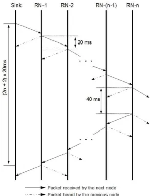
Prior to run SRNMS in the network, all relay nodes should be synchronized to determine which window they will send and receive message from others. This synchronization is done by passing synchronization packet, which contains counting number of relay node, to the end of relay node. After reaching the end of relay node, the packet will be send back to the sink to start superframe for message scheduling. For better understanding, the illustration of relay node synchronization is given in Figure 3.
In the figure 3, every time window for transmitting synchronization packet is set to be 20 ms following the size of time slot used in this scheme. When synchronization packet arrives back at the sink, the end to end delay can be calculated which happens to be (2n + 2) multiplied by 20 ms. In this synchronization part, 40 ms is added for ensuring whether next node exist or not. The absence of next node is detected by the inability of last node to hear packet from next node.
After getting information regarding the number of relay nodes, each node will calculate the superframe size and determine which window or time slot they will send or
receive message. The size of superframe is calculated by neglecting every possibility of collision among all relay nodes. To elaborate the way to calculate superframe, the study case of relay node is given in Figure 4.
Figure 3 Timing diagram of Relay Synchronization
Figure 4 Example of relay node in the network
Suppose, RN-1 sends message to sink which can also be heard by RN-2. In that condition, collision occur either RN-2 sends message to RN-1 or RN-3 sends message to RN-2 as already explained at the previous section. However, the collision will not occur when RN-4 sends message to RN-3. Due to that fact, RN-1 and RN-4 can send message at the same time. The same condition can be applied to RN-2 which makes RN-2 and RN-5 can send message at the same time.
Table 2 Transmission Restriction of Relay Nodes Sender
Node
Interference
Sink RN-1 RN-2 RN-3 RN-4
RN-5
Sink 0 1 1 0 0 0
RN-1 1 0 1 1 0 0
RN-2 0 1 0 1 1 0
RN-3 0 1 1 0 1 1
RN-4 0 0 1 1 0 1
RN-5 0 0 0 1 1 0
In order to calculate the size of superframe, it is necessary to consider the following rules.
• Sink node also acts as the coordinator that transmits beacon message to synchronize all relay nodes. The power transmission may also be amplified to reach all relay nodes
• There is no simultaneous slot occupation with beacon time slot. It is because beacon time slot is used for synchronization or broadcast information to all relay nodes.
• Relay node can only reach direct neighbor relay nodes as explained before. For example, 2 can only reach RN-1 and RN-3.
• Time slot occupation after beacon time slot should be done consecutively. For example, first time slot is occupied by RN-1, second time slot is occupied by RN-2, and so on. Further explanation about assigning time slot is given in Algorithm 1.
• Number of simultaneous slot Nss at a super frame is calculated as :
N
ss=
N
max−
RN
3
,
(2)Algorithm 1. Creating superframe for synchronized relay node message scheduling
1.MaxRNode = N;
2.RNode=1; simRNode=1; TSlot = 1;
3.for RNode = 1 to MaxRNode do
4.if RNode is not assigned time slot then Assign
RNode to TSlot;
5.end if
6.for simRNode = RNode + 1 to MaxRNode do
7.if RNode and simRNode have no interference then
Assign simRNode to TSlot;
8.end if
9.end for
10.TSlot = TSlot + 1;
11.end for
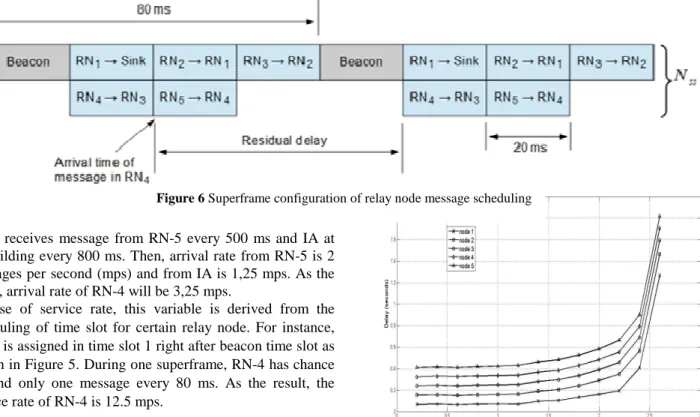
which Nmax−RN is total number of RN in the network. For five relay nodes as shown in Figure 4, the time slot configuration is given in Figure 5. In that figure, every time slot is associated with certain relay node and its transmission direction. Second row time slots depict the simultaneous message transmission which is conducted by two relay nodes, e.g. relay node 1 and 4, that are not interfering each others as given in Table II.
3.2 Delay Calculation on Relay Nodes Based Network
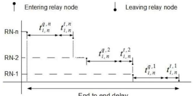
End to end delay calculation is created by observing the travel of one message from certain node to the sink. For example, RN-5 in Figure 4. receives message Mi
5 , from the
Figure 5 End to end delay of a message in relay node based
network
plant layer (IA) at building 5 at which i is index of message. Right after arriving at RN-5, Mi5 will enter transmission queue/buffer which is assumed to be very huge size or closed to infinity in this case for simplicity. As the consequence, there is no buffer over flow or message drop in the system in case of arrival rate of the message is bigger than the service rate of the relay node system. After leaving transmission queue, Mi5 will be transmitted to the next node which is closer to the sink (RN-4). At that relay node, Mi5 will also entering transmission buffer for certain times until all messages in front of Mi
5
are sent to the next node. All this procedures are repeated sink as shown in Figure 6.
Then, the formula of end to end delay of a message ti,n eed
as shown in Figure 6 can be constructed as follows.
t
i,need=
t
i,nq, j+
t
i,nt, jj=n
1
∑
,
(3) which ti,n
eed
and ti ,n t , j
mean queueing delay and transmission time of Min at relay node-j respectively.
By modelling end to end delay of that relay node based network using queueing theory [11], the new formula can be derived as follows.
t
i,need
=
t
i,nq, j
1
−
ρ
j+
t
i,n t , jj=n
1
∑
,
(4) which
t
i,nq, j
and ρ mean average residual delay of
M
i nat node-j and utilization of the system respectively. Residual delay is the delay experienced by that message prior to arrive at assigned time slot in the superframe as shown in Figure 5. For simplicity, this paper assumes that residual delay of all messages follow uniform distribution which is equal to half of superframe size (40 ms). Utilization of the system can be derived from the comparison between arrival rate and service rate of the system which is
t
i,need=
t
i,nq, j+
t
i,nt , jj=n
1
RN-4 receives message from RN-5 every 500 ms and IA at its building every 800 ms. Then, arrival rate from RN-5 is 2 messages per second (mps) and from IA is 1,25 mps. As the result, arrival rate of RN-4 will be 3,25 mps.
In case of service rate, this variable is derived from the scheduling of time slot for certain relay node. For instance, RN-4 is assigned in time slot 1 right after beacon time slot as shown in Figure 5. During one superframe, RN-4 has chance to send only one message every 80 ms. As the result, the service rate of RN-4 is 12.5 mps.
4.
Simulation
Simulation environment in this paper is built in C code by using GCC compiler with topology as shown in Figure 4. Messages in the network are generated by plant layer with certain message rates. Those messages have to be delivered to the sink by using synchronized relay node message scheduling as explained in the previous section through relay nodes based network.
The bit rate used in each relay node is set to be 9600 bps. The size of data used in each message is 16 bytes including the header of message which contains source and destination address and also other message control bytes. The reason behind this small size of data is becasuse industrial network requires small data exchange which contain status or control data periodically. As the consequence, the size of time slot for each relay node and the size of superframe are 20 ms and 80 ms respectively as already explained in the previous section.
4.1 Performance Result and Evaluation
In this subsection, delay characteristic and throughput of relay node based network are evaluated in detail. To exploit the performance of this relay node based network, workloads, which are generated from plant layer, with different rate (mes- sages per second) are given. Those workloads are generated periodically which follow normal distribution from 0.2 mps to 3.0 mps.
ρ
j=
λ
jµ
j,
(5)
Figure. 7 Average end to end delay on relay node scheme
The result for delay measurement on each relay node is given in Figure 7. Based on that figure, as the distance between relay node and sink increases, the end to end delay from that relay node to the sink also increases. This result occurs due to the increasing number of transmission needed to deliver a message to the sink as shown in Figure 6. As an example, message end to end delay of RN-5, at plant layer traffic 0.2 mps, is bigger than message end to end delay of RN-4 which is 0.4 seconds and 0.32 seconds respectively.
In other aspect, the end to end delay from all relay nodes increases slowly as the plant layer traffic increases. This result happens because of increasing number of the messages in the buffer of each relay node. As the result queueing delay at each relay nodes increases and affects the end to end delay of each message as already given in Equation 3.
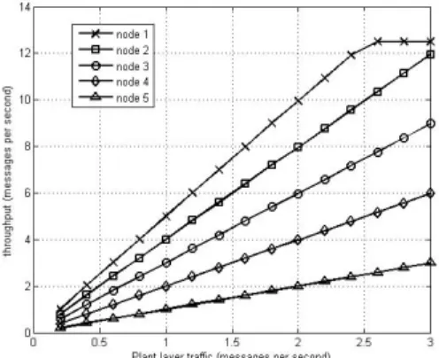
There is one point in Figure 7 at which end to end delay of each relay node starts to increase dramatically. This result happens due to the throughput bottleneck at RN-1 to the sink as given in Figure 8. The fact that throughput of RN-1 to the sink goes constantly (around 12.5 mps) from plant layer traffic generation 2.6 mps shows the existence of link congestion which leads to increasing of queueing delay occurring in relay node 1. As the consequence, end to end delay of all messages increase dramatically because all messages should travel through RN-1 prior to arrive at the sink.
Figure 8 Throughput on each relay node
5.
Conclusions and Future Work
This paper presented a network extension on industrial plant for monitoring production process using low rate wireless sensor network. This network extension in this paper is developed by using relay node based network which transmits message to the next relay nodes and sink synchronously and simultaneously. Based on simulation results, the end to end delay of each relay node message is affected by the distance between relay node to the sink and also the plant layer traffic which is used as the workloads for this simulation. The bottleneck in this relay node based network happens in RN-1 which creates dramatic increase of message end to end delay from each relay node. For the future work, we will try to improve this relay node scheme method by employing other famous protocol such as ISA100.11a or Wireless HART and combine TDMA based and CSMA based approach.
References
[1] X. feng Wan, Y.-S. Xing, and L. xiang Cai, “Application and implemen- tation of can bus technology in industry real-time data communication,” in Industrial Mechatronics and Automation, 2009. ICIMA 2009. International Conference on, May 2009, pp. 278–281.
[2] E. Joelianto and Hosana, “Performance of an industrial data communication protocol on ethernet network,” in Wireless and Optical Communications Networks, 2008. WOCN ’08. 5th IFIP International Conference on, May 2008, pp. 1–5. [3] H. Z. Abidin, N. M. Din, N. A. M. Radzi, “Deterministic Static
Sensor Node Placement in Wireless Sensor Network based on Territorial Predator Scent Marking Behavior”, International Journal of Communication Networks and Information Security Vol. 5, No. 3, pp. 186-191, 2013.
[4] Franco Frattolillo, “A Deterministic Algorithm for the Deployment of Wireless Sensor Networks”, International Journal of Communication Networks and Information Security Vol. 8, No. 1, pp. 1-10, 2016.
[5] H. Hayashi, T. Hasegawa, and K. Demachi, “Wireless technology for process automation,” in ICCAS-SICE, 2009, aug. 2009, pp. 4591 –4594.
[6] N. Baker, “Zigbee and bluetooth strengths and weaknesses for industrial applications,” Computing Control Engineering Journal, vol. 16, no. 2, pp. 20 –25, april-may 2005.
[7] K. Al Agha, M.-H. Bertin, T. Dang, A. Guitton, P. Minet, T. Val, and J.-B. Viollet, “Which wireless technology for industrial wireless sensor networks? the development of ocari technology,” IEEE Transactions on Industrial Electronics, vol. 56, no. 10, pp. 4266 –4278, oct. 2009.
[8] I. Akyildiz and M. C. Vuran, Wireless Sensor Networks. New York, NY, USA: John Wiley & Sons, Inc., 2010.
[9] F. Dewanta, F. Rezha, and D.-S. Kim, “Message scheduling approach on dedicated time slot of isa100.11a,” in ICT Convergence (ICTC), 2012 International Conference on, Oct 2012, pp. 466–471.
[10]Y. Chung, K. hyung Kim, and S. wha Yoo, “Time slot schedule based minimum delay graph in tdma supported wireless industrial system,” in international Conference on Computer Information Systems and Industrial Management Applications (CISIM), 2010, oct. 2010, pp. 265–268.
[11]A. Koubaa, R. Severino, M. Alves, and E. Tovar, “Improving quality- of-service in wireless sensor networks by mitigating hidden-node colli- sions,” IEEE Transactions on Industrial Informatics, vol. 5, no. 3, pp. 299–313, Aug 2009.
[12]S.-T. Sheu, Y.-Y. Shih, and W.-T. Lee, “Csma/cf protocol for ieee 802.15.4 wpans,” IEEE Transactions on Vehicular Technology, vol. 58, no. 3, pp. 1501–1516, March 2009. [13]D.Bertsekas and R.Gallager, Data Networks second