Munich Personal RePEc Archive
Time-Varying Vector Autoregressions:
Efficient Estimation, Random Inertia and
Random Mean
Legrand, Romain
24 August 2019
Online at
https://mpra.ub.uni-muenchen.de/95707/
Time-Varying Vector Autoregressions: Efficient
Estimation, Random Inertia and Random Mean
Romain Legrand
∗This version: September 2018
Abstract
Time-varying VAR models have become increasingly popular and are now widely used for policy analysis and forecast purposes. They constitute fundamental tools for the anticipation and anal-ysis of economic crises, which represent rapid shifts in dynamic responses and shock volatility. Yet, despite their flexibility, time-varying VARs remain subject to a number of limitations. On the theoretical side, the conventional random walk assumption used for the dynamic parameters appears excessively restrictive. It also conceals the potential heterogeneities existing between the dynamic processes of different variables. On the application side, the standard two-pass proce-dure building on the Kalman filter proves excessively complicated and suffers from low efficiency.
Based on these considerations, this paper contributes to the literature in four directions: i) it introduces a general time-varying VAR model which relaxes the standard random walk as-sumption and defines the dynamic parameters as general auto-regressive processes with variable-specific mean values and autoregressive coefficients.
ii) it develops an estimation procedure for the model which is simple, transparent and efficient. The procedure requires no sophisticated Kalman filtering methods and reduces to a standard Gibbs sampling algorithm.
iii) as an extension, it develops efficient procedures to estimate endogenously the mean values and autoregressive coefficients associated with each variable-specific autoregressive process. iv) through a case study of the Great Recession for four major economies (Canada, the Euro Area, Japan and the United States), it establishes that forecast accuracy can be significantly improved by using the proposed general time-varying model and its extensions in place of the traditional random walk specification.
JEL Classification: C11, C15, C22, E32, F47.
Keywords: Time-varyings coefficients; Stochastic volatility; Bayesian methods; Markov Chain Monte Carlo methods; Forecasting; Great Recession.
1
Introduction
VAR models have become the cornerstone of applied macroeconomics. Since the seminal work of Sims (1980), they have been used extensively by financial and economic institutions to perform routine policy analysis and forecasts. While convenient, VAR models with static coefficients and residual variance often turn out to be excessively restrictive in capturing the dynamics of time-series, which often exhibit some form of non-linearity in their behaviours. This motivated the introduction of time-varying coefficients in VAR models (Doan et al. (1983), Canova (1993), Stock and Watson (1996), Cogley (2001), Ciccarelli and Rebucci (2003)), along with stochastic volatility (Harvey et al. (1994), Jacquier et al. (1995), Uhlig (1997), Chib et al. (2006)), and more recently both features (Cogley and Sargent (2005), Primiceri (2005)), in order to account for potential shifts in the transmission mechanism and volatility of the underlying structural shocks.
Since then, time-varying VAR models have become increasingly popular. They have been used for a wide range of applications related to policy analysis, including the evolution of monetary policy over the last decades (Primiceri (2005), Mumtaz and Zanetti (2013), Korobilis (2013)), the response to exchange rate movements (Mumtaz and Sunder-Plassmann (2010), Kavtaradze and Mokhtari (2018), Abbate and Marcellino (2018b)), the impact of fiscal policy (Gerba and Hauzenberger (2013), Eisenstat et al. (2016)), or the general analysis of macroeconomic fluctua-tions (Gali and Gambetti (2008), Koop and Korobilis (2012)). Time-varying vector autoregres-sions have also become a benchmark for forecasting as a well-established literature demonstrates that they generally perform better than their static counterparts (Clark (2011), D’Agostino et al. (2011), Aastveit et al. (2017), Abbate and Marcellino (2018a)).
Lately, time-varying VAR models have received much attention regarding the analysis and an-ticipation of economic crises, in particular the events of the Great Recession. The literature has considered two main classes of explanations for this episode of severe economic decline. The first view focuses on the heteroskedasticity of the exogenous shocks (Stock and Watson (2012), Doh and Connolly (2013), Bijsterbosch and Falagiarda (2014), Gambetti and Musso (2017)). It interprets the Great Recession primarily as an episode of sharp volatility of the structural dis-turbances affecting the economy. The second view emphasizes the changes in the transmission mechanism (Baumeister and Benati (2010), Benati and Lubik (2014), Ellington et al. (2017) among many others). It considers the Great Recession essentially as a period of altered response of macroeconomic variables to economic policy. In either case, there is strong evidence that modelling time variation adequately is important to the accuracy of both policy analysis and forecasts in a context of crisis. In this respect, it seems plausible that the Great Recession could have been better apprehended with a proper use of time-varying VAR models. Time-varying VARs may also constitute a benchmark tool in the future to predict economic downturns and accurately forecast their evolutions.
On the theoretical side, the first limitation consists in the choice of a random walk specification for the laws of motion of the different dynamic parameters. This formulation has been widely adopted by the literature, both for the VAR coefficients and the log volatilities of the structural shocks. Though convenient for its simplicity and parsimony, it may be inconsistent with the behaviour of the data. A random walk implies that the range of values taken by the dynamic parameters of the model increases over time and becomes eventually unbounded, resulting in an explosive behaviour in the limit. This is at odd with both empirical observations and economic theory such as the notion of balanced growth path. Most importantly, it is unlikely that such a formulation proves appropriate to describe the short-term fluctuations of economic data. For in-stance, a well-known feature of the random walk is that it grants equal weight to all past shocks. But if an economy experiences rapid shifts in its dynamics due to a series of large disturbances, as would be the case in a context of crisis, it becomes crucial to capture correctly the effect of the most recent shocks while granting less weight to past shocks. This supposes the use of more gen-eral formulations, possibly stationary and mean-reverting, in place of the standard random walk.
The random walk specification is further criticisable as it results de facto in a homogeneity as-sumption. It indeed implies that all the dynamic parameters follow a similar unit-root process. There is yet no legitimate reason to assume that the dynamic parameters of different variables evolve homogenously. In fact, it is quite likely that different economic variables are characterised by different behaviours of their dynamic coefficients and residual volatilities. Following, the state equations of the parameters should be formulated on a variable-specific basis to account for the potential heterogeneities prevailing from one variable to another.
While switching from a homogeneous random walk specification to a set of variable-specific sta-tionary processes is conceptually trivial, it complicates the estimation procedure. Perhaps for this reason, and even though such alternative formulations have attracted considerable attention in the univariate ARCH literature (Jacquier et al. (1994), Kim et al. (1998), Chib et al. (2002), Jacquier et al. (2004), Eisenstat and Strachan (2016), among others), the contributions on the multivariate side are considerably more limited. Doan et al. (1983) consider a general stationary formulation for the VAR coefficients of their model, but set the autoregressive coefficient to0.999, which effectively turns the formulation into a random walk. Ciccarelli and Rebucci (2003) and Lubik and Matthes (2015) also propose a general stationary formulation for the law of motion of their time-varying VAR models, but retain the random walk for empirical applications. Clark and Ravazzolo (2015) test for different specifications of stochastic volatility in VAR models, in-cluding a stationary autoregressive specification. Their results with the competing random walk formulation are overall inconclusive.
random walk specification. Nevertheless, he does not include a mean term in the autoregressive processes and does not adopt an variable-specific formulation, which may significantly affect the results. Mumtaz and Zanetti (2013) endogenously estimate a single autoregressive coefficient on stochastic volatility, assumed to be common to all the structural shocks.
Aside from theoretical considerations, estimation remains the main challenge for time-varying VAR models. Except for a marginal number of contributions building on frequentist methods (Gorgi et al. (2017)), the Bayesian approach has been unanimously adopted by the literature for its flexibility. So far the benchmark methodology relies on the state-space formulation proposed by Primiceri (2005), building on the algorithm developed by Carter and Kohn (1994). The technique involves a two-pass procedure. It starts with an initial forward filtering pass making use of the Kalman filter to produce recursively the predictive mean for each period, followed by a subsequent backward filtering pass drawing the states in reverse order. A first limit of the procedure resides in its complexity. The use of multiple filtering stages combined with the general Kalman filter approach makes the technique complicated to understand and implement. It also limits the transparency and intuitiveness of the procedure.
A second concern comes for the efficiency of the process. The multiple loops through time and the building of the states in a recursive fashion considerably slow down the procedure. It is not uncommon for time-varying Bayesian VARs to be estimated in hours or even days. This significantly reduces the attractiveness of the model, feasibility remaining a key factor in empir-ical applications. In this respect, an important contribution was made by Chan and Jeliazkov (2009). These authors propose to replace the usual state-space resolution method with a pre-cision sampler based on a full sample formulation. Despite its efficiency, the procedure has remained confidential and applications have been limited. Poon (2018) expands the approach to time-varying panel VAR models, using a structural factor approach, while Chan and Eisenstat (2018) expand the use of the precision sampler to the estimation of the structural identification matrix. These preliminary expansions remain nevertheless limited. First, they only extend the precision sampler to a fraction of the parameters involved in the model. Second, the dynamic parameters remain defined by the standard random walk approach. Third, the formulation of the precision sampler is not optimised, resulting in reduced efficiency benefits.
predicted with a proper use of time-varying VAR models. In this respect, this paper adds to a growing literature discussing the optimal specification of time-varying VAR models regarding forecast accuracy (Clark and Ravazzolo (2015), Aastveit et al. (2017), Kalli and Griffin (2018)).
The remaining of the paper is organised as follows: section 2 introduces the general time-varying model and provides the details of the estimation procedure; section 3 discusses the efficiency of the procedure compared to the usual state-space formulation, along with alternative estima-tion strategies for the stochastic volatility components of the model; secestima-tion 4 and 5 respectively develop the extensions allowing for endogenous estimation of the autoregressive coefficients (ran-dom inertia) and mean terms (ran(ran-dom mean) of the dynamic parameters; section 6 presents the results of the case study on the Great Recession and discusses the benefits of the general time-varying model and its extensions in terms of forecast accuracy; section 7 concludes.
2
A general time-varying model
2.1 The model
Consider the general time-varying model:
yt=Ctzt+A1,tyt−1+· · ·+Ap,tyt−p+εt t= 1,· · ·, T , εt∼ N(0,Σt) (1)
ytis a n×1 vector of observed endogenous variables, zt is am×1 vector of observed exogenous
variables such as constant or trends, andεtis an×1 vector of reduced-form residuals.1 The
resid-uals are heteroskedastic disturbances following a normal distribution with variance-covariance matrixΣt. Ct, A1,t,· · ·, Ap,t are matrices of time-varying VAR coefficients comfortable with zt
and the lagged values ofyt. Stacking in a vectorβt the set of VAR coefficients, (1) rewrites:
yt=Xtβt+εt (2)
with:
Xt=In⊗xt , xt= zt′ y
′
t−1 · · · y ′
t−p
, βt=vec(Bt) , Bt= Ct A1,t · · · Ap,t
′
(3)
Considering specifically rowiof (2), the equation for variablei of the model rewrites:
yi,t =xtβi,t+εi,t (4)
where βi,t is the k×1 vector obtained from column i of Bt. Stacking (4) over the T sample
periods yields a full sample formulation for variablei:
Yi =Xβi+Ei (5)
with:
Yi =
yi,1
yi,2
.. . yi,T
, X =
x1 0 · · · 0
0 x2 . .. ...
..
. . .. ... 0 0 · · · 0 xT
, βi=
βi,1
βi,2
.. . βi,T
, Ei =
εi,1
εi,2
.. . εi,T (6) 1
Unlike Primiceri (2005) and part of the literature, the model is introduced in reduced form rather than as a structural VAR. There are a number of reasons for doing so, including intuitiveness and flexibility in the implementation of a potential structural decomposition. The correspondence between the two formulations is neverthless straightforward, as the matrix ∆−1
The variance-covariance matrixΣt for the reduced form residuals is decomposed into:
Σt= ∆tΛt∆′t (7)
∆tis a unit lower triangular matrix, and Λt is a diagonal matrix with positive diagonal entries,
taking the form:
∆t=
1 0 · · · 0
δ21,t 1 . .. ...
..
. . .. . .. 0
δn1,t · · · δn(n−1),t 1
, Λt=
s1 exp(λ1,t) 0 · · · 0
0 s2 exp(λ2,t) . .. ...
..
. . .. . .. 0
0 · · · 0 sn exp(λn,t)
(8)
The decomposition of the variance-covariance matrixΣt implemented in (9) is common in
time-series models (see for instance Hamilton (1994)). The coefficients in∆tandΛtcan be respectively
interpreted as the covariance and volatility components of Σt. Thesi terms are positive scaling
hyperparameters which represent the equilibrium value of the diagonal entries ofΛt. For technical
reasons which will become clear later, it is more convenient to work with∆−1
t than with∆t. The
transformation is harmless since there is a one-to-one correspondence between the two terms. As∆t is unit lower triangular, so is∆
−1
t :
∆−1
t =
1 0 · · · 0
δ−1
21,t 1 . .. ...
..
. . .. . .. 0
δ−1
n1,t · · · δ
−1
n(n−1),t 1 (9)
Denoting by δ−1
i,t the vector of non-zero and non-one terms in row i of ∆
−1
t so that δ
−1
i,t =
(δ−1
i1,t · · · δ
−1
i(i−1),t) ′
, δ−1
i,t represents the (inverse) residual covariance terms of variable i with
the other variables of the model.
The dynamics of the model’s time varying parameters is specified as follows:
βi,t = (1−ρi)bi+ρiβi,t−1+ξi,t t= 2,3, . . . , T ξi,t∼ N(0,Ωi)
βi,1 =bi+ξi,1 t= 1 ξi,1 ∼ N (0, τΩi)
λi,t=γiλi,t−1+νi,t t= 2,3, . . . , T νi,t ∼ N(0, φi)
λi,1 =νi,1 t= 1 νi,1∼ N (0, µφi)
δ−1
i,t = (1−αi)di−1+αiδi,t−1−1+ηi,t t= 2,3, . . . , T ηi,t ∼ N(0,Ψi)
δ−1
i,1 =d
−1
i +ηi,1 t= 1 ηi,1 ∼ N(0, ǫΨi) (10)
ρi,γi and αi represent variable-specific autoregressive coefficients while bi,si and d−i 1 represent
for the greater uncertainty associated with the initial period.
All the innovations in the model are assumed to be jointly normally distributed with the following assumptions on the variance covariance matrix:
V ar εt ξi,t νi,t ηi,t =
Σt 0 0 0
0 Ωi 0 0
0 0 φi 0
0 0 0 Ψi
(11)
This concludes the description of the model. The parameters of interest to be estimated are: the dynamic VAR coefficients βi = {βi,t :i = 1, . . . , n;t = 1, . . . , T}, the dynamic volatility terms
λi = {λi,t : i= 1, . . . , n;t = 1, . . . , T}, the dynamic inverse covariance terms δ
−1
i = {δ
−1
i,t :i=
2, . . . , n;t = 1, . . . , T}, and the associated variance-covariance parameters Ωi, φi and Ψi. To
these six base parameters must be added an additional parameterri={ri,t :i= 1, . . . , n;
t= 1, . . . , T}, whose role will be clarified shortly.
2.2 Bayes rule
Following most of the litterature on time-varying VAR models, Bayesian methods are used to evaluate the posterior distributions of the parameters of interest. Given the model, Bayes rule is given by:
π(β,Ω, λ, φ, δ−1
,Ψ, r|y)∝f(y|β, λ, δ−1
, r)
×
n
Y
i=1
π(βi|Ωi)π(Ωi)
! n Y
i=1
π(λi|φi)π(φi)
! n Y
i=2
π(δ−1
i |Ψi)π(Ψi)
! n Y
i=1 T
Y
t=1
π(ri,t)
!
(12)
2.3 Likelihood function
A standard formulation of the likelihood function can be obtained from (2):
f(y|β, λ, δ−1
, r) =
T
Y
t=1
(2π)−n/2
|Σt|−1/2exp
−1
2(yt−Xtβt)
′
Σ−1
t (yt−Xtβt)
(13)
(13) does not permit to estimate the different parameters of the model since it is not expressed in variable-specific terms. After some manipulations, it reformulates as:
f(y|β, λ, δ−1
, r) = (2π)−nT /2
n
Y
i=1
s−i T /2
!
exp −1
2
n
X
i=1
λ′
i1T
!
× exp −1
2
n
X
i=1
s−1
i
n
(Yi−Xβi)
′˜
Λi(Yi−Xβi) + (E−iδ −1
i )
′˜
Λi(E−iδ −1
i ) + 2(Yi−Xβi)
′˜
Λi(E−iδ −1
i )
o !
with:
λi=
λi,1
λi,2
.. . λi,T
, 1T =
1 1 .. . 1
, Λ˜i=
exp(−λi,1) 0 · · · 0
0 exp(−λi,2) . .. ...
..
. . .. . .. 0
0 · · · 0 exp(−λi,T)
E−i = ε′
−i,1 0 · · · 0
0 ε′
−i,2 . .. ...
..
. . .. ... 0 0 · · · 0 ε′
−i,T
, ε−i,t =
ε1,t
ε2,t
.. .
εi−1,t
, δ−1
i =
δ−1
i,1
δ−1
i,2
.. .
δ−1
i,T (15)
(14) proves convenient for the estimation of βi and δi−1, but does not provide any conjugacy
for λi due to the presence of the exponential term ˜Λi. This is a well-known issue of models
with stochastic volatility, and the most efficient solution is the so-called normal offset mixture representation proposed by Kim et al. (1998).2 The procedure consists in reformulating the likelihood function in terms of the transformed shock et = (∆tΛ1t/2)
−1
εt. It is trivially shown
thatet is a vector of structural shock withet∼ N(0, In). Considering specifically the shockei,t
in the vector, squaring, taking logs and rearranging eventually yields:
ˆ
ei,t= log(e2i,t) = ˆyi,t−λi,t yˆi,t = log
s−1
i (εi,t+δ−i,t1
′
ε−i,t)2
(16)
ˆ
ei,t follows a log chi-squared distribution which does not grant any conjugacy. Kim et al. (1998)
thus propose to approximate the shock as an offset mixture of normal distributions. The ap-proximation is given by:
ˆ
ei,t≈ 7
X
j=1
✶(ri,t =j)zj , zj ∼ N(mj, vj) , P r(ri,t =j) =qj (17)
The values for mj, vj and qj can be found in Table 4 of Kim et al. (1998). The constants mj
and vj respectively represent the mean and variance components of the normally distributed
random variablezj. ri,t is a categorical random variable taking discrete valuesj = 1, . . . ,7,the
probability of obtaining each value being equal toqj. Finally,✶(ri,t=j) is an indicator function
taking a value of 1 if ri,t = j, and a value of 0 otherwise. To draw from the log chi-squared
distribution, the mixture first randomly draws a value for ri,t from its categorical distribution;
onceri,t is known, its value determines which component zj of the mixture is selected. eˆi,t then
turns into a regular normal random variable with meanmj and variancevj. Given (16) and the
offset mixture (17), an approximation of the likelihood function obtains as:
f(y|β, λ, δ−1
, r) =
n Y i=1 T Y t=1 7 X j=1
✶(ri,t=j)
(2πvj)
−1/2
exp
−1
2
(ˆyi,t−λi,t−mj)2
vj
(18)
For the estimation of λi, a more convenient joint formulation can be adopted. Defining ri =
(ri,1 . . . ri,T)′, denoting by J any possible value for ri, by mJ and vJ the resulting mean and
variance vectors, and defining VJ = diag(vJ), the likelihood function rewrites as a mixture of
multivariate normal distributions:
2
f(y|β, λ, δ−1
, r)
= n Y i=1 J X
✶(ri =J)
(2π)−T /2
|VJ|−1/2exp
−1
2( ˆYi−λi−mJ)
′
V−1
J ( ˆYi−λi−mJ)
(19)
with: ˆ
Yi = ˆyi,1 yˆi,2 . . . yˆi,T
′
=log(s−1
i Qi) Qi = (Ei+E−iδ −1
i )2 (20)
2.4 Priors
The formulation of the priors for the dynamic parameters obtains from a generalisation of the procedure by Chan and Jeliazkov (2009). Consider first the VAR coefficients βi. Starting from
(10), the law of motion can be expressed in compact form as:
Ik 0 · · · 0
−ρiIk Ik . .. ...
..
. . .. . .. 0 0 · · · −ρiIk Ik
βi,1
βi,2
.. . βi,T = bi
(1−ρi)bi
.. . (1−ρi)bi
+
ξi,1
ξi,2
.. . ξi,T (21) or:
(Fi⊗Ik) βi = ¯bi+ξi Fi=
1 0 · · · 0
−ρi 1 . .. ...
..
. . .. ... 0 0 · · · −ρi 1
¯
bi =
bi
(1−ρi)bi
.. . (1−ρi)bi
ξi =
ξi,1
ξi,2
.. . ξi,T (22) Also:
V ar(ξi) =
τΩi 0 · · · 0
0 Ωi . .. ...
..
. . .. ... 0 0 · · · 0 Ωi
=Iτ⊗Ωi Iτ =
τ 0 · · · 0
0 1 . .. ... ..
. . .. ... 0 0 · · · 0 1
(23)
(22) and (23) respectively implyβi = (Fi⊗Ik)−1¯bi+ (Fi⊗Ik)−1ξi andξi∼ N(0, Iτ⊗Ωi). From
this and rearranging, the prior distribution eventually obtains as:
π(βi|Ωi)∼ N (βi0 ,Ωi0) βi0 = 1T ⊗bi Ωi0 = (Fi′ I
−1
τ Fi⊗Ω−i 1)
−1
(24)
Using forλi and δ
−1
i equivalent procedures and notations, it is straightforward to obtain:
π(λi|φi)∼ N (0,Φi0) Φi0 =φi(G′iI
−1
µ Gi)−1
π(δ−1
i |Ψi)∼ N δ
−1
i0 ,Ψi0
δ−1
i0 = 1T ⊗d
−1
i Ψi0 = (H
′
i I
−1
ǫ Hi⊗Ψ−i 1)−1 (25)
Once the prior distributions for the dynamic parameters are determined, it remains to set the priors for their associated variance-covariance parameters. The choice is that of standard inverse Wishart and inverse Gamma distributions. Precisely:
π(Ωi)∼IW (ζ0,Υ0) π(φi)∼IG
κ0
2 ,
ω0
2
π(Ψi) ∼IW (ϕ0,Θ0) (26)
Finally, from (17), it is immediate that the prior distribution forri,t is categorical:
2.5 Posteriors
The joint posterior obtained from (12) is analytically intractable. Following standard practices, the marginal posteriors are then estimated from a Gibbs sampling algorithm relying on condi-tional distributions.
For βi, Bayes rule (12) implies π(βi|y, β−i) ∝ f(y|β, λ, δ −1
, r)π(βi|Ωi).3 From the likelihood
(14), the prior (24) and rearranging, it follows that:
π(βi|y, β−i)∼ N( ¯βi,Ω¯i) with:
¯ Ωi =
s−1
i X
′˜
ΛiX+Fi′ I
−1
τ Fi⊗Ω−i 1
−1
¯
βi = ¯Ωi
s−1
i X
′˜
Λi
Yi+E−iδ −1
i
+F′
iI
−1
τ Fi1T ⊗Ω
−1
i bi
(28)
For λi, Bayes rule (12) implies π(λi|y, λ−i) ∝ f(y|β, λ, δ −1
, r)π(λi|φi). From the approximate
likelihood (19), the prior (25) and rearranging, it follows that:
π(λi|y, λ−i)∼ N(¯λi,Φ¯i) with:
¯ Φi = (V
−1
J +φ
−1
i G
′
iI−µGi)
−1 ¯
λi= ¯Φi(V
−1
J [ ˆYi−mJ]) (29)
Forδ−1
i , Bayes rule (12) impliesπ(δ
−1
i |y, δ
−1
−i)∝f(y|β, λ, δ −1
, r)π(δ−1
i |Ψi). From the likelihood
(14), the prior and rearranging, it follows that:
π(δ−1
i |y, δ
−1
−i) ∼ N(¯δ −1
i ,Ψ¯i) with:
¯ Ψi= (s
−1
i E
′
−iΛ˜iE−i+H ′
i I−ǫ Hi⊗Ψ −1
i )
−1
¯
δ−1
i = ¯Ψi(−s−i1E
′
−iΛ˜iEi+H ′
iI−ǫHi1T ⊗Ψ −1
i d
−1
i ) (30)
Consider now the associated variance-covariance parameters. For Ωi, Bayes rule (12) implies
π(Ωi|y,Ω−i)∝π(βi|Ωi)π(Ωi). From the priors (24) and (26) then rearranging, it follows that:
π(Ωi|y,Ω−i)∼IW(¯ζ,Υ¯i) with: ζ¯=T +ζ0 Υ¯i = ˜Bi+ Υ0
˜
Bi = (Bi−1′T ⊗bi) (Fi′ I−τ Fi)(Bi−1 ′
T ⊗bi)′ Bi = (βi,1 βi,2 · · · βi,T) (31)
Forφi, Bayes rule (12) impliesπ(φi|y, φ−i)∝π(λi|φi)π(φi). From the priors (25) and (26) then
rearranging, it follows that:
π(φi|y, φ−i)∼IG(¯κ,ω¯i) with: ¯κ=
T +κ0
2 ω¯i =
λ′
i(G
′
iI−µGi)λi+ω0
2 (32)
For Ψi, Bayes rule (12) impliesπ(Ψi|y,Ψ−i) ∝π(δ −1
i |Ψi)π(Ψi). From the priors (25) and (26)
then rearranging, it follows that:
π(Ψi|y,Ψ−i) ∼IW( ¯ϕ,Θ¯i) with: ϕ¯=T +ϕ0 Θ¯i = ˜Di+ Θ0
˜
Di= (Di−1
′
T ⊗d
−1
i ) (H
′
i I−ǫ Hi)(Di−1 ′
T ⊗d
−1
i )
′
Di = (δ
−1
i,1 δ
−1
i,2 · · · δ
−1
i,T) (33)
Finally, for ri,t, Bayes rule (12) implies π(ri,t|y, r−i,t) ∝ f(y|β, λ, δ −1
, r)π(ri,t). From the
ap-proximate likelihood (18) and the prior (27), it follows immediately that:
π(ri,t|y, r−i,t)∼Cat(¯q1, . . . ,q¯7) with: q¯j = (2πvj) −1/2
exp
−1
2
(ˆyi,t−λi,t−mj)2
vj
qj (34)
3
Forθiany parameter,π(θi|θ−i) is used to denote the density ofθiconditional on all the model parameters except
2.6 MCMC algorithm
Once the conditional posteriors are obtained, it is possible to introduce the MCMC algorithm for the model. The latter reduces to a simple 7-step procedure, as follows:
Algorithm 1: MCMC algorithm for the general time-varying model:
1. Sampleλi from π(λi|y, λ−i)∼ N(¯λi,Φ¯i).
2. Sampleβi from π(βi|y, β−i)∼ N( ¯βi,Ω¯i).
3. Sampleδ−1
i fromπ(δ
−1
i |y, δ
−1
−i)∼ N(¯δ −1
i ,Ψ¯i).
4. SampleΩi fromπ(Ωi|y,Ω−i)∼IW(¯ζ,Υ¯i).
5. Sampleφi fromπ(φi|y, φ−i)∼IG(¯κ,ω¯i).
6. SampleΨi fromπ(Ψi|y,Ψ−i)∼IW( ¯ϕ,Θ¯i).
7. Sampleri,t from π(ri,t|y, r−i,t)∼Cat(¯q1, . . . ,q¯7).
Two remarks can be made about the algorithm. First, observe that the ordering of the steps in the algorithm differs from the one used for the presentation of the model. It introducesλi first,
then the other model parameters, and eventually the offset mixture parameterri,t. This specific
ordering is necessary to recover the correct posterior distribution if the normal offset mixture is used to provide an approximation of the likelihood function. See Del Negro and Primiceri (2015) for details. Second, due to the large dimension of βi andδ−i 1, it is not advisable nor efficient to
compute explicitly the parameters ¯βi,Ω¯i,δ¯i−1 and ¯Ψi defining the normal distributions. A better
option consists in taking advantage of the sparse and banded nature of ¯Ω−1
i and ¯Ψ
−1
i to proceed
efficiently by backward and forward substitution. See Chan and Jeliazkov (2009), Algorithm 1 for details.
3
Efficiency analysis
3.1 Estimation
As a preliminary exercise and for the sake of comparison, the methodology introduced in section 2 is used to estimate the small U.S. economy model of Primiceri (2005). The data set includes 3 variables: a series of inflation rate and unemployment rate representing the non-policy block, and a short-term nominal interest rate representing the policy block. Estimation is conducted with two lags and one constant on quarterly data running from 1963q1 to 2001q3, resulting in a sample of sizeT = 153 quarters.
For the priors, one possibility consists in calibrating the hyperparameters with a training sample, as done by Primiceri (2005). Since there is no evidence that such a strategy improves on the esti-mates, simple values are used instead. For the inverse Wishart priors on the variance-covariance hyperparameters Ωi and Ψi, the degrees of freedom are set to a small value of 5 additional to
set to Υ0 = 0.01Ik and Θ0 = 0.01Ii−1. Combined with the degrees of freedom, this implies
an average 0.05 standard deviation for the shocks on the dynamic processes, or in other words a 5% difference between consecutive values of βi and δ−i 1. For the stochastic volatility part of
the model, the prior is slightly looser. The shape and scale parameters of the inverse Gamma prior distribution on φi are set to κ0 = 1 andω0= 0.01 to generate a weakly informative prior.
Finally, the initial period variance scaling terms are set to τ = µ= ǫ = 5 in order to obtain a variance over the initial periods which is roughly equivalent to that prevailing for the rest of the sample. For the dynamic processes, the autoregressive coefficients are set toρi=γi=αi = 0.9,
inducing stationarity but a susbtantial degree of inertia. For the mean of the dynamic processes, static OLS estimates are used. bi is set to its OLS counterpart ˆβi. Similarly, the static OLS
estimate ˆΣ is decomposed into ˆΣ = ˆ∆ˆΛ ˆ∆′
. si is then set as theith diagonal entry of ˆΛ, andd−i 1
is determined as the free elements of theith row of ˆ∆−1
. The model is run from 10000 iterations of the MCMC algorithm, discarding the initial 2000 iterations as burn-in sample. As shown in Appendix A, The convergence diagnostics are satisfactory, indicating proper convergence to the posterior distribution.
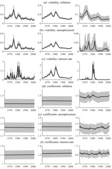
To highlight the main characteristics of the model, Figure 1 compares the results obtained with the methodologies of Primiceri (2005) (left panels, without corrigendum), Del Negro and Prim-iceri (2015) (middle panels, integrating the corrigendum), and the general time-varying model (right panels).4 The three top panels report the historical evolution of the volatility of the
struc-tural shocks while the three bottom panels focus on the developments of the dynamic coefficients (own first lag of each variable).
On the qualitative side, the different models produce comparable outcomes in terms of shock volatility. For inflation and unemployment, the three models detect an initial fuelling in volatility somewhere around 1975 followed by a moderate recurrence in the course of the 1980’s. For the interest rate, the three models adequately identify the high volatility peak occurring in 1982. Interestingly enough, the results obtained with the general time-varying model are qualitatively closer to those obtained from the original Primiceri (2005) model than to those provided by the corrigendum model by Del Negro and Primiceri (2015) which are considerably smoother. The conclusion concerning the VAR coefficients are quite different: while the estimates from the general time-varying model display a significant amount of variation accross the sample, those produced by the two comparative models are virtually flat.
4
Figure 1: Median and 70% credibility interval for the volatility and VAR coefficients (own first lag) of inflation, unemployment and the interest rate left panels: Primiceri (2005) (no corrigendum), middle panels: Del Negro and Primiceri
The explanation comes from the quantitative side of the models. The three top panels reveal that the overall range of volatility induced by the general time-varying model is considerably smaller than with the other models. This is true for all the variables, despite the higher peak in volatility for the interest rate in 1982. This is a consequence of the inclusion of the variable-specific mean terms si in the dynamic processes of stochastic volatility, as stated in (8). This sets si as
the prior equilibrium value of the process, which drives by construction the posterior towards it. By contrast, the log-normal random walk formulations of Primiceri (2005) and Del Negro and Primiceri (2015) effectively amount to scaling the means to si = 1 for all the variables.
This normalisation of the prior equilibrium is not innocuous as it pushes the posterior estimates upward, resulting in higher levels of fluctuation. As a consequence, most of the variation observed in the data is attributed to stochastic volatility. This leaves only a marginal extent of variation to be explained by the dynamic coefficients, hence the remarkably flat estimates. On the other hand, because the stochastic volatility contributions of the general time-varying model remain modest, a larger share of the observed data variability is left to be explained by the dynamic VAR coefficients, hence the wider range of fluctuation. Overall, these conclusions question the common belief that time-varying models attribute the bulk of observed fluctuations to stochastic volatility, while the dynamic responses play a marginal role. This feature may in fact be a technical artefact produced by the random walk assumption, which disappears once a more general formulation is adopted.
3.2 Efficiency
This section discusses the computational efficiency of the general time-varying model compared to the standard Primiceri (2005) methodology, integrating the corrigendum of Del Negro and Primiceri (2015). To do so, three models are considered. The first is the model developed in the previous section, labeled as the “small” model. As a reminder, the model includes three variables (inflation, unemployment and interest rate), two lags and runs from 1963q1 to 2001q3, which represents an estimation sample of 153 quarters. The second is an abridged version of the small model which contains only two variables (inflation and unemployment), one lag, and runs for a smaller period ranging from 1980q1 to 2001q3, resulting in an estimation sample of 86 quarters. This is labelled as the “tiny” model. The final “medium” model to be estimated is an expanded version of the initial model. It comprises four variables (inflation, unemployment and interest rate supplemented with a series of real GDP growth), three lags and covers a longer period ranging from 1953q1 to 2018q1, for a total of 218 quarters. Table 1 reports the approx-imate estimation time to achieve 10000 iterations with the Primiceri (2005) methodology and the general time-varying model 5. The table reveals significant efficiency gains from using the general time-varying model methodology. The computational benefits range from about 55% for the medium model to more than 90% for the tiny model. For a typical small-sized time-varying model like the small US economy model of Primiceri (2005), the computational gain is greater than 80%. Clearly, the returns are diminishing with the number of parameters to be estimated. The benefit remains however considerable even when the number of parameters is quite large, as in the case of the medium model. In fact, for any reasonably sized time-varying VAR model, the benefit will remain sizable.
5
Number of estimated parameters
Methodology of Primiceri (2005)
General time-varying
model Efficiency gain
[image:16.595.95.500.103.173.2]Tiny model 774 558 s (9 m 18 s) 51 s (0 m 51 s) 90.9 % Small model 4131 1186 s (19 m 46 s) 218 s (3 m 38 s) 81.6 % Medium model 16132 2650 s (44 m 10 s) 1195 s (19 m 55 s) 54.9 %
Table 1: Summary of estimation performances for the different methodologies (for 10000 iterations; time in seconds)
There are two main sources for the observed efficiency gains. The first consists in the adoption of the precision sampler of Chan and Jeliazkov (2009) in place of the usual Kalman filter procedure of Carter and Kohn (1994) for drawing the dynamic parameters βi, λi and δi−1. The benefit
from the procedure is double: while the standard approach proceeds period by periods and re-quires a two-pass filtering process, the precision sampler draws for all the periods at once from the highly multivariate posterior distribution of each parameter. The efficiency of the method depends on the size of the matrices involved (seeFi, Iτ−1,Ωi, Gi, I−µ, Hi, I−ǫ andΨi in (28), (29)
and (30)) which themselves depend on the dimension of the modeln, the number of coefficients per equationk, as well as the number of sample periodsT. Larger matrices involve a more than linear increase in the number of computations and result in a relative loss of efficiency, though the number of calculations evolve at less than a square rate due to the sparse and banded nature of ¯Ω−1
i ,Φ¯
−1
i and ¯Ψ
−1
i . It is then not surprising that the benefit from the precision sampler gets
smaller as the overall number of parameters increases, even though it remains substantial for any reasonable model.
The second source of gains lies in the optimised formulation of the precision sampler. While Chan and Jeliazkov (2009) and Chan and Eisenstat (2018) realise the computations at the largest scale, the present model is formulated to take advantage of the Kronecker structure of the formulas, allowing to work at a smaller scale. For instance, the computation of the posterior parameter ¯Ω−1
i in (28) only involves the update of the k×k matrix Ω
−1
i at each iteration of
the MCMC algorithm, which is then enlarged through the Kronecker productF′
i I
−1
τ Fi⊗Ω−i 1,
whereF′
i I
−1
τ Fi is a constant term which needs only to be computed once, prior to the initiation
of the algorithm. By contrast, Chan and Jeliazkov (2009) explicitly re-compute the whole term (Fi ⊗ Ik)(Iτ ⊗Ωi)−1(Fi ⊗Ik) at every iteration,6 which involves products and inversions of
matrices of size T k×T k. Also, rather than relying on the simple parameter τ to determine the distribution of the first period, these authors create an additional step which endogenously estimate an initial condition for period 0. While the gains from these formulations may sound modest, they eventually add up to generate substantial benefits once applied to all the dynamic parameters and repeated over thousands of iterations. 7
6
In fact, the term computed by Chan and Jeliazkov (2009) is only an equivalent of (Fi⊗Ik)(Iτ⊗Ωi)−
1
(Fi⊗Ik),
the formulation of their model being slightly different from the present general time-varying model.
7
3.3 Alternative estimation strategies
The main difficulty in the estimation of time-varying models comes from the standard log-normal formulation of the stochastic volatility processes. This assumption results in a likelihood function containing double exponential stochastic volatility terms such as the ˜Λi matrices in (14). These
terms are challenging and prevent any conjugacy with a normal prior distribution for λi. The
solution adopted for the general time-varying model is the normal offset mixture strategy of Kim et al. (1998). While it yields a convenient reformulation of the likelihood function, it also involves the estimation of the extra set of parameters ri which is undesirable as it generates
additional computations which contribute to reduce efficiency. It is thus important to consider alternative estimation strategies which may prove more efficient. To introduce the alternative solutions, observe first that the likelihood function (14) can rewrite as:
f(y|β, λ, δ−1
, r) = (2π)−nT /2
n
Y
i=1
s−i T /2
!
exp −1
2 n X i=1 n λ′
i1T +s−i1˜λ
′
i Qi
o !
(35)
where ˜λi = (exp(−λi,1) exp(−λi,2) · · · exp(−λi,T))′. Clearly, ˜λi is the equivalent of ˜Λi in
(14). It constitutes the log normal term which generates the difficulties in obtaining analytical forms for the posterior distribution of λi. Indeed, Bayes rule (12) implies that π(λi|y, λ−i) ∝
f(y|β, λ, δ−1
, r)π(λi|φi); substituting then for (35) and (25) and rearranging eventually yields:
π(λi|y, λ−i)∝exp
−1
2
n
λ′
i1T +s
−1
i λ˜
′
i Qi+λ
′
iΦ
−1
i0 λi
o
(36)
This cannot be reformulated as a multivariate normal density due to the presence of ˜λi. As
such, this posterior density is not workable. Besides the normal offset mixture approach of Kim et al. (1998), the literature has provided two classes of solutions for this issue. The first consists in the adoption of an accept-reject algorithm approach, while the second relies on the Metropolis-Hastings methodology. Both strategies can be applied either for all the sample peri-ods simultaneously, or on a period-by-period basis.
Consider first the accept-reject approach. This strategy was advocated for model with stochastic volatility by Kim et al. (1998). Noting that the problematic term ˜λi in (36) can be approximated
by a first-order Taylor series around 0 as ˜λi =exp(−λi)≥1T −λi, where the inequality follows
from the convexity of ˜λi, one obtains:
π(λi|y, λ−i) ∝exp
−1
2
n
λ′
i1T +s−i 1λ˜
′
i Qi+λ′iΦ
−1
i0 λi
o ≤exp −1 2 λ′
i1T +s−i 1(1T −λi)′ Qi+λ′iΦ
−1
i0 λi
∝exp
−1
2(λi−λ¯i)
′
Φ−1
i0 (λi−λ¯i)
(37)
with:
¯
λi= 1
2Φi0(s
−1
The final row of (37) is immediately recognisable as the kernel of a multivariate normal den-sity. In other words, the actual posterior density (36) is dominated by a simple multivariate normal density. A natural accept-reject approach thus consists in drawing a candidate value from λi ∼ N(¯λi,Φi0), and then accept it with a probability equal to the ratio of the actual
density to the candidate density, given by p(a) = exp−1 2s
−1
i (˜λi+λi−1T)Qi
. If the can-didate is rejected, a new cancan-didate is considered until acceptance is obtained. In theory, the algorithm can be very efficient, especially if the acceptance rate is high. The additional benefits are obvious: unlike the offset mixture approach, the accept-reject approach does not involve the estimation of any additional random variables; the formulas involved in the algorithm are trivial to compute; also, efficiency is maximised from the fact that in case of rejection, a new candidate is immediately drawn until acceptance is achieved.
In practice however, the algorithm works poorly and often ends up being trapped repeatedly at the rejection stage. There are two main explanations for this situation. The first is the quality of the approximation provided by the dominating function: a poor approximation results in low acceptance rates, except if the candidate is drawn very close to the approximation point. For the considered application, it is clear that the first-order Taylor series ˜λi ≈1T −λi constitutes
only a crude approximation. The second explanation lies in the dimensionality of the target distribution: a high dimension contributes to reduce the acceptance rate of the algorithm as the distances between the actual and candidate distributions add up over the dimensions. It is in fact a well-known property that the acceptance probability of any accept-reject algorithm falls to zero as the dimensionality of the candidate distribution approaches infinity. Due to its high dimensionality of T, the joint accept-reject approach for λi becomes quickly inefficient.
In an attempt to suppress the dimensionality issue, one may opt for a period-by-period approach. From Bayes rule (12), the likelihood function (35), the prior (25), a Taylor approximation and some rearrangement, one obtains:8
π(λi,t|y, λ−i−t) ∝exp −
1 2
(
λi,t+s−i 1λ˜i,t Qi,t+(
λi,t−ˆλi,t)
ˆ
φi
)!
≤exp
−1
2
(λi,t−¯λi,t)
¯
φi
(39)
with:
¯
φi= ˆφi =
φi
1 +γ2 i
¯
λi,t= ˆλi,t+
¯
φi
2(s
−1
i Qi,t−1) λˆi,t =
γi
1 +γ2 i
(λi,t−1+λi,t+1) (40)
Following, a period-by-period accept-reject procedure consists in drawing a candidate value from
λi,t∼ N(¯λi,t,φ¯i) and accept it with probabilityp(a) =exp
−1 2s
−1
i (˜λi,t+λi,t−1)Qi,t
. While this procedure yields slightly better results than the simultaneous period approach, its perfor-mance remains poor. Even though the dimensionality issue is settled, the approximation remains too rough and the acceptance probability stays close to zero.9 In the end, the accept-reject ap-proach proves unsuccessful, except in the case of extremely tight priors for λi which generate
candidates close to zero, the point of approximation. Consequently, it does not represent a viable alternative to the offset mixture approach in general.
8
The values are slightly different for the initial and final periods and are omitted to save space.
9
The second class of methodologies relies on the Metropolis-Hastings approach. This strategy was proposed by Cogley and Sargent (2005) for multivariate models with stochastic volatility. A first possibility consists in adopting a joint period approach. Notice that (36) can rewrite as:
π(λi|y, λ−i)∝exp
−1
2
n
λ′
i1T +s−i 1λ˜
′
i Qi
o exp −1 2λ ′ iΦ −1
i0 λi
(41)
The first term on the right-hand side represents the contribution of the data, while the second represents the prior distribution. A simple strategy consists in drawing a candidate from the prior (the second term) and then confront it to the data (the likelihood contribution) to decide on acceptance or rejection.10 Specifically, this defines an independent transition kernel which yields an acceptance probability of:
p(a) =exp
−1
2{(λ
(n) i −λ
(n−1)
i )
′
1T +s−i 1(˜λ (n) i −λ˜
(n−1)
i )
′
Qi}
(42)
whereλ(in−1)denotes the value inherited from the previous iteration, andλ(in)denotes the candi-date at iterationn. If the candidate is rejected, the value from the previous iteration is retained. The advantage of this Metropolis-Hastings algorithm lies in the simplicity of the approach and the formulas involved in the calculations. On the other hand, a well-known drawback of such algorithm is that it produces repeated values at rejection, which often leads to increase the number of iterations or implement thinning of the draws to reduce the autocorrelation of the chain. In the case of the multivariate approach developed here, however, the prime concern is the failure to reach the posterior distribution. Because the candidates are drawn from the prior distribution, they may only partially cover the posterior distribution. Following, even though the accepted values belong to the posterior, the full distribution will not be recovered except if the prior fully overlaps with the posterior, which is not generally true.
For this reason, it is preferable to follow a period-by-period approach. Observe that (39) may rewrite:
π(λi,t|y, λ−i−t) ∝exp
−1
2
n
λi,t+s−i 1˜λi,t Qi,t
o
exp −1
2
(λi,t−ˆλi,t)
ˆ
φi
!
(43)
The procedure then consists in drawing a candidate from the the second term and use the first term to decide on acceptance or rejection. This again defines an independent transition kernel which yields an acceptance probability of:
p(a) =exp
−1
2{(λ
(n) i,t −λ
(n−1)
i,t ) +s
−1
i (˜λ (n) i,t −˜λ
(n−1)
i,t )Qi,t}
(44)
The main difference between the multivariate approach and the period-by-period approach is that in the latter the candidates are not drawn from the prior distribution. As can be seen from (40), the mean value ˆλi,t of the candidate distribution involves λi,t−1 and λi,t+1 which
come directly from the posterior distribution. For this reason, a period-by-period algorithm will properly converge to the posterior distribution and cover its whole support.
10
Alternatively, one may draw the candidates from exp −1 2
λ′
i1T+λ′iΦ−
1
i0 λi rearranged as a multivariate
normal density, and use the remaining term exp−1 2
n
s−1
i λ˜′i Qi
o
In terms of efficiency, the performances of the algorithm are satisfactory. On the one hand, the iterative scheme of the procedure makes it intrinsically slower than the offset mixture method-ology, but on the other hand the omission of the additional parameterri permits to spare some
computations. In the end, the two algorithms are roughly equivalent on a per iteration basis. Also, the concern that Metropolis-Hastings produces repeated values is not to bee taken too seriously in this case: empirical applications suggest that the acceptance rate of the procedure typically exceeds 80%, which produces only few repetitions. The only significant difference be-tween the two approaches resides in the number of iterations required for convergence. While the offset mixture typically obtains convergence in 2000 iterations or so, the Metropolis-Hastings al-gorithm is more sluggish and requires between 5000 and 10000 iterations to achieve convergence. This is due to the recursive nature of the algorithm which only allows for small moves of the chain for each sample period, the amplitude being restricted by the neighbouring values. In the end, the offset mixture approach remains the most efficient method, though the period-by-period Metropolis-Hastings algorithm constitutes an acceptable alternative.
4
Random inertia
In the basic version of the general time-varying model, the autoregressive coefficientsρi, γi and
αi associated with the dynamic processes in (10) are treated as exogenous hyperparmeters. The
traditional choice in the literature consist in setting ρi =γi =αi = 1 which corresponds to the
homogeneous random walk assumption. Rather, the calibration proposed for the general time-varying model usesρi =γi =αi= 0.90, which reduces the inertia of the process and attributes
some weight to the mean component. While this choice is reasonable and preferable to the usual random walk specification, it is in not necessarily optimal. For this reason, this section proposes a simple procedure to estimate endogenously the autoregressive coefficientsρi, γi andαi.
4.1 Priors
The literature has produced a number of options to define the prior distributions of autoregressive coefficients. On the univariate side, the Beta distribution has sometimes been favoured for its support producing values between zero and one (Kim et al. (1998)). The Beta is however not conjugate with the normal distribution, which leads to an inefficient Metropolis-Hastings step in the estimation. On the multivariate side, a simpler alternative has consisted in using normal distributions (Primiceri (2005), Mumtaz and Zanetti (2013)). The prior is diffuse to let the data speak and produce posteriors centered on OLS estimates. While simple, this strategy is unadvisable for two reasons. First, as the support of the normal distribution is unrestricted, part of the posterior distribution may lie outside of the zero-one interval, which is not meaningful from an economic point of view. Second, the use of a diffuse prior is suboptimal as relevant information can be introduced at the prior stage. For these reasons, the prior is chosen here to be a truncated normal distributions with informative hyperparameters. Considering for instanceρi in (10), the
prior distribution is a normal distribution with mean ρi0 and variance πi0, truncated over the
[0 1] interval:
π(ρi)∼ N[0 1](ρi0, πi0) (45)
0.01. This way, the prior is sufficiently loose to allow for significant differences in the posterior distributions of the differentρi’s, but also sufficiently restrictive to avoid posteriors that would be
too far away from the prior and implausible. Finally, the truncation operated at the prior stage ensures that the posterior distribution is restricted over the same range [0 1], effectively ruling out irrelevant parts of the support. A similar strategy is applied to the other autoregressive coefficients in (10):
π(γi)∼ N[0 1](γi0, ςi0) π(αi)∼ N[0 1](αi0, ιi0) (46)
The mean and variance parameters are set to γi0=αi0 = 0.8 and ςi0 =ιi0 = 0.01.
4.2 Bayes rule
Bayes rule must be slightly amended due to the inclusion of ρi, γi and αi as random variables.
The updated version obtains as:
π(β,Ω, ρ, λ, φ, γ, δ−1
,Ψ, α, r|y)∝f(y|β, λ, δ−1
, r)
n
Y
i=1
π(βi|Ωi, ρi)π(Ωi)π(ρi)
!
×
n
Y
i=1
π(λi|φi, γi)π(φi)π(γi)
! n Y
i=2
π(δ−1
i |Ψi, αi)π(Ψi)π(αi)
! n Y
i=1 T
Y
t=1
π(ri,t)
!
(47)
4.3 Posteriors
As for the basic model, the marginal posteriors are estimated from a Gibbs sampling algorithm re-lying on conditional distributions. Forρi, Bayes rule (47) impliesπ(ρi|y, ρ−i)∝π(βi|Ωi, ρi)π(ρi).
From the priors (24) and (45) and some rearrangement, it follows that:
π(ρi|y, ρ−i)∼ N[0 1](¯ρi,π¯i) with:
¯
πi = ( ¨βi,t′ −1β¨i,t−1+π −1
i0 )
−1
¯
ρi= ¯πi( ¨βi,t′ −1β¨i,t+π −1
i0 ρi0)
¨
βi,t =vec(Ω
−1/2
i
′
(βi,2−bi · · · βi,T −bi)) (48)
For γi, Bayes rule (47) implies π(γi|y, γ−i) ∝ π(λi|φi, γi)π(γi). From the priors (25) and (46)
and some rearrangement, it follows that:
π(γi|y, γ−i)∼ N[0 1](¯γi,ς¯i) with:
¯
ςi = (¨λ′i,t−1λ¨i,t−1+ς −1
i0 )
−1
¯
γi = ¯ςi(¨λ′i,t−1λ¨i,t+ς −1
i0 γi0)
¨
λi,t=φ
−1/2
i (λi,2 . . . λi,T)
′
(49)
Finally forαi, Bayes rule (47) implies π(αi|y, α−i) ∝ π(δ −1
i |Ψi, αi)π(αi). From the priors (25)
and (46) and some rearrangement, it follows that:
π(αi|y, α−i)∼ N[0 1](¯αi,¯ιi) with:
¯ιi= (¨δ
−1
i,t−1 ′¨
δ−1
i,t−1+ι −1
i0 )
−1
¯
αi = ¯ιi(¨δ
−1
i,t−1 ′¨
δ−1
i,t +ι
−1
i0 αi0)
¨
δ−1
i,t =vec(Ψ
−1/2
i
′
(δ−1
i,2 −d
−1
i · · · δ
−1
i,T −d
−1
i )) (50)
4.4 MCMC algorithm
The Markov Chain Monte Carlo algorithm for the model with random inertia is fundamentally similar to the one of the general time-varying model. The 7 steps of Algorithm 1 are thus un-changed, but 3 additional steps specific to the model must be inserted between steps 6 and 7:
Algorithm 2: additional steps of the MCMC algorithm for the model with random inertia:
1. Sampleρi from π(ρi|y, ρ−i)∼ N[0 1](¯ρi,π¯i).
2. Sampleγi from π(γi|y, γ−i)∼ N[0 1](¯γi,ς¯i).
3. Sampleαi from π(αi|y, α−i)∼ N[0 1](¯αi,¯ιi).
5
Random mean
The standard version of the general time-varying model treats the mean parameters bi, si and
d−1
i in (8) and (10) as exogenously supplied hyperparameters. While simple, this assumption
may be overly restrictive. In particular, the preliminary conclusions obtained from Figure 1 suggest that the mean terms may be of considerable importance as they determine the share of data variation endorsed by each component of the model (dynamic coefficients, stochastic volatility and residual covariance). Endogenous estimation then constitutes a natural extension. While the univariate ARCH literature has paid some attention to this question in the context of stochastic volatility processes (Jacquier et al. (1994), Kim et al. (1998)), the subject has been almost completely neglected in multivariate models. One notable exception is the contribution of Chiu et al. (2015) who integrate a (period-specific) mean component to the dynamic variance of the residuals. This section fills the gap by proposing simple estimation procedures for the mean components of the dynamic processes.
5.1 Priors
Forbi, the choice for the prior is that of a simple multivariate normal distribution with meanbi0
and variance-covariance matrixΞi0:
π(bi)∼ N(bi0,Ξi0) (51)
In the basic version of the general time-varying model, bi is set according to its static OLS
estimate ˆβi, which constitutes a reasonable starting point. For this reason, the prior mean bi0
is set to ˆβi while the prior standard deviation is set to a fraction ̟i of this value, resulting in
Ξi0 = diag((̟iβˆi)2). Small values of ̟i generate a tight and hence informative prior around
ˆ
βi while larger values can be used to achieve diffuse and uninformative priors. Given the lack of
Similar strategies are applied for si and d−i 1. For the si which are positive scaling terms, the
inverse Gamma represents a natural candidate. Specifically, the prior for each si is inverse
Gamma with shapeχi0 and scaleϑi0:
π(si)∼IG
χi0
2 ,
ϑi0
2
(52)
The hyperparameter values χi0 and ϑi0 are then chosen to imply a prior mean of sˆi, the OLS
estimate used for the general time-varying model, and a prior standard deviation equal to a fraction ψi of this value.11 . As a base case, ψi is set to 0.25 in order to generate, again, an
informative but sufficiently loose prior.
Finally, the prior for each d−1
i is multivariate normal with mean d
−1
i0 and variance-covariance
matrixZi0:
π(d−1
i )∼ N(d
−1
i0 , Zi0) (53)
The prior mean is set as d−1
i0 = ˆd
−1
i , the OLS estimate used for the general time-varying
model, and the the prior standard deviation is set to a fraction ̺i of this value, resulting in
Zi0= diag((̺idˆi−1)2). An informative but loose prior is achieved by setting ̺i = 0.25.
5.2 Bayes rule
Given the model, the updated version of Bayes rule is given by:
π(β,Ω, b, λ, φ, s, δ−1
,Ψ, d−1
, r|y)∝f(y|β, λ, s, δ−1
, r)
n
Y
i=1
π(βi|Ωi, bi)π(Ωi)π(bi)
!
×
n
Y
i=1
π(λi|φi)π(φi)
! n Y
i=1
π(si)
! n Y
i=2
π(δ−1
i |Ψi, d−i 1)π(Ψi)π(d−i1)
! n Y
i=1 T
Y
t=1
π(ri,t)
!
(54)
5.3 Posteriors
For bi, Bayes rule (54) implies π(bi|y, b−i) ∝ π(βi|Ωi, ρi)π(bi). From the priors (24) and (51)
and some rearrangement, it follows that:
π(bi|y, b−i)∼ N(¯bi,Ξ¯i) with:
¯
Ξi = ˜τiΩ−i 1+ Ξ
−1
i0
−1 ¯
bi= ¯Ξi Ω−i1(˜ρi⊗Ik)βi+ Ξ−i01bi0
˜
τi =τ−1+ (1−ρi)2(T −1) ρ˜i= τ−1−(1−ρi)ρi (1−ρi)2 · · · (1−ρi)2 (1−ρi)
(55)
Forsi, Bayes rule (54) implies π(si|y, s−i)∝f(y|β, λ, s, δ −1
, r)π(si). From the likelihood
func-tion (35), the prior (52) and some rearrangement, it follows that:
π(si|y, s−i)∼IG( ¯χi,ϑ¯i) with:
¯
χi =
T +χi0
2 ϑ¯i =
˜
λ′
i Qi+ϑi0
2 (56)
11
Finally for d−1
i , Bayes rule (54) impliesπ(d
−1
i |y, d
−1
−i)∝π(δ −1
i |Ψi, d−i 1)π(d
−1
i ). From the priors
(25) and (53) and some rearrangement, it follows that:
π(d−1
i |y, d
−1
−i)∼ N( ¯d −1
i ,Z¯i) with:
¯
Zi = ˜ǫiΨ−i 1+Z
−1
i0
−1
¯
d−1
i = ¯Zi Ψ−i 1(˜αi⊗Ii−1)δ −1
i +Z
−1
i0 d
−1
i0
˜ǫi=ǫ−1 +(1−αi)2(T −1) α˜i= ǫ−1 −(1−αi)αi (1−αi)2 · · · (1−αi)2 (1−αi)
(57)
The other posteriors are unchanged.
5.4 MCMC algorithm
The Markov Chain Monte Carlo algorithm for the model with random mean is fundamentally similar to the one of the general time-varying model. The 7 steps of Algorithm 1 are thus un-changed, but 3 additional steps specific to the model must be inserted between steps 6 and 7:
Algorithm 3: additional steps of the MCMC algorithm for the model with random mean:
1. Samplebi fromπ(bi|y, b−i) ∼ N(¯bi,Ξ¯i).
2. Samplesi from π(si|y, s−i) ∼IG( ¯χi,ϑ¯i).
3. Sampled−1
i from π(d
−1
i |y, d
−1
−i)∼ N( ¯d −1
i ,Z¯i).
6
A case study on the Great Recession
6.1 Setup
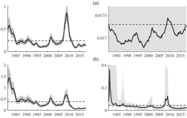
The aim of the exercise consists in assessing the forecast performances of different models for key periods of the crisis. Figure 2 displays the growth rate of GDP 12 for the four considered economies over the Great Recession periods. For each country, three critical periods of the crisis are considered. The first period is the recession period, the period at which the country enters into negative growth. For Canada, the Euro area, Japan and the United States, this respectively occurs in 2009q1, 2008q4, 2008q2 and 2008q3. The second period considered is the reversion period, the period at which GDP growth reaches its minimum before it starts increasing again. This respectively happens in 2009q3, 2009q1, 2009q1 and 2009q2. The final period considered is the recovery period, the period at which the economy hits positive growth again. For the four countries considered, this happens in 2010q1. These periods are of special importance for policy makers as they corresponds to the points where the crisis respectively initiates, reverts and ends. It is crucial to anticipate them correctly in order to provide an adequate answer to the rapidly changing economic conditions.
2005q1 2005q3 2006q1 2006q3 2007q1 2007q3 2008q1 2008q3 2009q1 2009q3 2010q1 2010q3 2011q1 2011q3 2012q1 2012q3
-8 -4 0 4 8
[image:25.595.107.491.290.544.2]Canada Euro area Japan United States
Figure 2: Year-on-year GDP growth for the four major economies
The forecasting exercise is performed in pseudo real time, that is, it does not use information which is not available at the time the forecast is made. For this reason, for each country and each considered period of the crisis the model is estimated from 1971q1 up to the period preceding the forecast period. The forecast is then obtained as the one period-ahead out-of-sample prediction. For each forecast, two criteria are considered. The first criterion is the classical Root Mean Squared Error (RMSE) which considers the accuracy of point forecasts. Denoting by y˜t+h the
h-step ahead prediction and by yt+h the realised value, it is defined as:
12
RM SEt+h=
s
1
h
h
Σ
i=1(˜yt+h−yt+h)
2 (58)
The second criterion is the Continuous Ranked Probability Score (CRPS) of Gneiting and Raftery (2007) which evaluates density forecasts. As pointed by those authors, this criterion presents advantages over alternative density scores such as the log score as it rewards more density points close to the realised value and is less sensitive to outliers. Denoting byF the cumulative distribution function of the h-step ahead forecast density and by yˆt+h and yˆt′+h independent
random draws from this density, the CRPS is defined as:
CRP St+h=
Z ∞
−∞
(F(x)−✶(x≥yt+h))2dx=E|yˆt+h−yt+h| −
1
2E|yˆt+h−yˆ
′
t+h| (59)
Empirical estimations of the CRPS use the second term on the right-hand side of (59), ap-proximated from the Gibbs sampler draws. For both criteria, a lower score indicates a better performance.
Finally, the exercise considers five competing models. The first model is the homogenous random walk (Hrw) specification of Primiceri (2005), which obtains as a special case of the general time-varying model by setting the autoregressive coefficients of the dynamic processes to ρi = γi =
αi = 1 for all i = 1,· · · , n.13 The second model is the general time-varying (Gtv) model
developed in section 2, following the calibration proposed in section 3.1. The third and fourth models respectively consist in the general time-varying model augmented by the random inertia (Ri) extension developed in section 4 and the random mean (Rm) extension developed in section 5. The last model combines the two extensions, thus adding both random inertia and random mean (Rim) to the general time-varying model.
6.2 Results
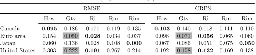
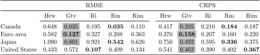
Table 2 reports the results of the experiment for unemployment. The results for inflation and the interest rate are fairly similar and relegated to Appendix B in order to save space. Table 2 comprises three parts: the top, middle and bottom panels which respectively correspond to forecast evaluations for the recession, reversion and recovery periods. In each panel, the left part summarizes the results for the RMSE while the right part reports the results for the CRPS. For each country and each criterion, the bold entry corresponds to the model achieving the best forecast performance among the five competitors. Also, a shaded entry for the general time-varying model (second entry) indicates that the model performs better than the homogenous random walk formulation (first entry). In total, the experiment considers three periods, three variables, four countries and two evaluation criteria for a total of 72 forecast evaluations, each carried on a set of five competing models.
13
Unemployment: recession period
RMSE CRPS
Hrw Gtv Ri Rm Rim Hrw Gtv Ri Rm Rim Canada 1.120 0.808 0.870 0.924 0.965 0.944 0.594 0.705 0.732 0.806 Euro area 0.299 0.291 0.331 0.316 0.339 0.198 0.185 0.231 0.212 0.235 Japan 0.