Tinbergen Institute Discussion Paper
Loyalty Programs and Consumer Behaviour:
The Impact of FFPs on Consumer Surplus
Christiaan Behrens
1Nathalie McCaughey
21 Faculty of Economics and Business Administration, VU University Amsterdam, and Tinbergen Institute, the Netherlands;
Rotterdam, the University of Amsterdam and VU University Amsterdam. More TI discussion papers can be downloaded at http://www.tinbergen.nl
Tinbergen Institute has two locations: Tinbergen Institute Amsterdam Gustav Mahlerplein 117 1082 MS Amsterdam The Netherlands Tel.: +31(0)20 525 1600 Tinbergen Institute Rotterdam Burg. Oudlaan 50
3062 PA Rotterdam The Netherlands Tel.: +31(0)10 408 8900 Fax: +31(0)10 408 9031
Duisenberg school of finance is a collaboration of the Dutch financial sector and universities, with the ambition to support innovative research and offer top quality academic education in core areas of finance.
DSF research papers can be downloaded at: http://www.dsf.nl/
Duisenberg school of finance Gustav Mahlerplein 117 1082 MS Amsterdam The Netherlands Tel.: +31(0)20 525 8579
on consumer surplus
$dr. Christiaan Behrensa,b,∗, dr. Nathalie C. McCaugheyc
aTinbergen Institute, Gustav Mahlerplein 117, 1082 MS Amsterdam, The Netherlands bDepartment of Spatial Economics, VU University Amsterdam, De Boelelaan 1105,
1081 HV Amsterdam, The Netherlands
cDepartment of Economics, Monash University, Victoria 3800, Australia
Abstract
Frequent Flier Programs (FFPs) are said to impact airline consumer behaviour such that revenue of sponsoring airlines increases. Prior research relies on aggregate industry data to study FFPs. We examine the impact of FFPs on individual consumer behaviour in a quasi-natural experimental set-up using a combined discrete choice and count data model. We exploit an unanticipated change in the FFP to avoid self-selection bias. We derive the causal effect of redesigning a frequency reward program into a customer tier program on average transaction size, purchase frequency, revenues of the sponsoring airline, and com-pensating variation. We find that, on average, revenues increased by 8US$ per member over a 16 month period. The welfare impact is small but positive. We find that, on av-erage, consumer surplus increased by 5US$ per member over a 16 month period. The re-sults vary substantially across individuals. In line with previous studies, our rere-sults sug-gest that moderate buyers increase their average transaction size and purchase frequency most due to the introduction of the customer tier program.
Keywords: Loyalty programs, Frequent Flier Programs, Two-stage budgeting model, Longitudinal demand models, Airline pricing
$This research is supported by Advanced ERC Grant OPTION # 246969 and NWO grant 400-08-102.
∗Corresponding author. Fax +31 20 5986004, phone +31 20 5984847. Email addresses: [email protected] (dr. Christiaan Behrens),
[email protected](dr. Nathalie C. McCaughey)
Introduction
Although initially derided as short-lived marketing gimmicks, Frequent Flier Programs (FFPs) matured from a narrowly targeted marketing device into an essential part of air-lines’ product offering. The significance of loyalty programs (LP) seems to be undoubted; over half of U.S. adults are enrolled in at least one LP and more than 120 million people are enrolled in one of the 200 airline LPs globally.
This article examines the impact of FFPs on individual consumer behaviour. We estimate a two-stage budgeting model with fare type choice and number of trips as dependent vari-ables in a quasi-natural experiment setting using negotiated access to the FFP database of a particular airline, hereafter called airline X.1 Subsequently, we use the estimation results
to identify and monetize the behavioural effect of the overnight change from a simple fre-quency reward program into a sophisticated customer tier program. To do so, we compare the actual transaction size, purchase frequency, revenues and consumer surplus with the hypothetical ones in which the new FFP would not have been implemented.
Revision of FFPs and inclusion of a tiered structure are a regular practice in the indus-try. For example, within the last three years, the US based airlines have revised their loy-alty programs three times. Despite the common practice and a growing body of literature, however, there is no evidence or consensus about the effectiveness and long term causal impact of these marketing strategies. This article provides a coherent analytical and em-pirical framework to support evidence-based marketing practices.
Using aggregate industry data, Lederman(2007, 2008) finds that (enhancements of) FFPs contribute to a price premium at hub airports, whereasMorrison et al. (1989) and Morri-son and Winston(1995) find a higher willingness to pay for air fares within a FFP. Baner-jee and Summers(1987) andBorenstein(1989) show that FFPs may affect competition negatively by raising entry barriers and switching costs. Switching costs, however, reduce
competition without necessarily making the firms better off (Klemperer,1987a,b). Basso et al.(2009) questions the effectiveness of FFPs and argues that with homogeneous prod-ucts such programs may increase competition.
Liu and Yang (2009), McCall and Voorhees (2010), and Dorotic et al.(2012) provide, amongst others, excellent reviews of the current research on LPs. In addition, Dorotic et al.(2012) andBreugelmans et al.(2014) formulate a research agenda to advance under-standing of such programs from both a scientific and practical point of view. Our article addresses three main themes mentioned in these research agendas: assessment of different LP structures (Breugelmans et al.,2014;Zhang and Breugelmans,2012), accounting for endogeneity and self-selection due to the participation decision (Breugelmans et al.,2014;
Leenheer et al.,2007), and differences in effectiveness across customer segments (Dorotic et al.,2012).
In August 2007, airline X changed its existing frequency reward program into a customer tier program. The new program includes three tier levels giving rise to an accelerated token accrual and priority treatments. In our quasi-experimental set-up, we exploit this change to assess the impact of implementing LP design changes. This set-up allows us to avoid the self-selection bias by looking only at already active members who initially qual-ify for the same tier level. Prior studies rely on longitudinal data (Liu, 2007) or dynamic modelling (Verhoef,2003;Lewis,2004) to alleviate this bias. These approaches, however, may not completely address the issue of self-selection, because there are no controls for the program participation decision. Our longitudinal data allows to address consumer het-erogeneity by estimating panel mixed logit models and poisson fixed effects models.
We model both dimensions of consumers’ usage levels, purchase frequency and fare type choice, in a two-stage budgeting model (Deaton and Muellbauer,1980;Hausman et al.,
1995;Hausman and Leibtag,2007;Rouwendal and Boter,2009). Most studies focus on purchase frequency as a LP performance measure, for example,Sharp and Sharp (1997),
Verhoef (2003), and Lewis(2004). Liu(2007) uses both measures as independent indica-tors and concludes that LPs positively affect both purchase frequency and transaction size for light and moderate buyers. The two-stage budgeting approach allows to quantify the impact of the LP design change on consumer well-being, measured as the compensating variation. To the best of our knowledge, this is the first attempt to quantify the impact of LP on consumers’ welfare. Both the size and sign of this impact are difficult to conjec-ture a priori, because this strategy combines elements of product differentiation and price discrimination.
On average, the impact of the change in LP design on consumer behaviour seems modest. We find an increase in average transaction size of 1 per cent to 113US$, and a decrease of 0.4 per cent, 4.5 flights, in number of flights. The change in consumer well-being is with, on average, 4.5US$, small but positive. The impact on total revenues is also positive, we find that airline X’s revenues increased by 8US$ per member over a 16 month period. In line with earlier studies, we find that accounting for unobserved heterogeneity improves es-timations. Huge variation across consumer segments is present. In particular those mem-bers who are in reach of qualifying for a next tier level, the moderate buyers, benefit most from the new FFP.
The remainder of this article is organised as follows. In the next section, we discuss our empirical strategy and introduce the data. We then set-up the two-stage budgeting model and provide the empirical specifications of the discrete choice and count data models. Subsequently, ww present the estimation results and discuss the implied impact on con-sumer behaviour. We conclude with a general discussion of our findings.
Identification Strategy and Data
In August 2007, airline X introduces its redesigned FFP overnight. From now on, mem-bers can qualify themselves for higher tier levels within the FFP based on their actual us-age level. We exploit this overnight change to identify the causal effect of tier levels on consumer behaviour. Because this change was not communicated beforehand, we avoid the standard issue of self-selection through endogenous participation decisions.
Our data set includes a 5 per cent stratified random sample of all active FFP members and contains all air and non-air related transactions in the period January 2006 to Decem-ber 2008. The stratification is based on the three memDecem-bership tier levels. To avoid any upward bias in the estimated impact of the change in the FFP, we only include members who qualify for the lowest tier level in August 2007.2 This group of light and moderate buyers, as referred to byLiu (2007), forms about 85% of all members in our data. We dis-tinguish between two periods, period 1 and 2: the year before and after the change in the FFP. This ensures that all individuals had a tier review exactly once within the new FFP. Furthermore, we select only those members who at least took one flight in one of the pe-riods. Our final sample contains 4,187 individuals and 43,576 trips over both periods, and includes a wide variety of trip and socio-economic characteristics, such as: fare type, price, days booked in advance, origin-destination, date, flight departure time, redemption be-haviour, place of residence, membership activation date, and job title.
Table 1shows the number of trips per fare type, period and trip purpose. Airline X of-fers a menu of four fare types. These fares range from lowest available to business flexible fare. The conditions attached to each type differ in, for example, luggage allowance and whether the ticket is transferable, refundable, or cancellable. The trip purpose is not di-rectly recorded in the data. We apply a set of rules to determine trip purpose. This set of rules can be found in Appendix A, together with detailed information about the
defini-tion and construcdefini-tion of the other variables. Table 1reveals that fare type 2 is, by far, the most chosen fare type in both periods for business and leisure trips. As one would expect, the share of more flexible and expensive fare types is higher for business trips suggesting a larger average transaction size for these trips.
Insert Table 1 about here
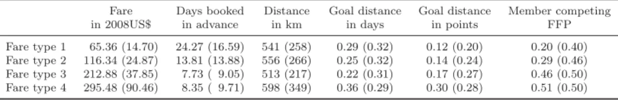
Table 2shows the mean and standard deviation of the main explanatory variables used in the transaction size model. The mean and standard deviation are specified per fare type. Intuitively, the average fare increases in flexibility and quality of the fare type. Further-more, these higher quality fare types are bought less days in advance. On the one hand, this might reflect that the lowest fare, fare type 1, is not available any more at the time of booking, whereas on the other hand it might reflect that members buying more expensive fare types, do not book far in advance. Table 2suggest that the average distance of a trip does not have such a clear pattern as the fare or days booked in advance.
Insert Table 2 about here
The remaining variables of interest concern loyalty programs. Airline X’s FFP is designed in such a way that token accrual is perfect linearly correlated with the fare: every member accrues a fixed number of tokens per dollar spent. For this reason, one cannot use directly the token accrual per trip as an explanatory variable. In order to identify the impact of tier and non-linear token accrual, in other words the new FFP, on consumer behaviour, we construct two extra variables. The variables are in line with the goal gradient hypoth-esis (Taylor and Neslin, 2005;Kivetz et al.,2006). The first variable indicates the number of days passed in the annual review period per booking; getting closer to the next review date leaves the member less time to accrue points to maintain his current tier level. The second variable indicates how, at the moment of booking, many points the member needs to qualify for the next tier level. The first variable is expressed as a fraction of the thresh-old level of points, whereas the latter one is a fraction of total days. Together, the
vari-ables capture the essence of the new FFP.3 Table 2shows a clear pattern for the goal
dis-tance in points: expensive fare types are bought by individuals who are closer to the next threshold level.
More than half of all airline X’s FFP members, 58 per cent, is also member of a compet-ing FFP. Approximately 80 per cent of these members have the lowest tier within that program, while the others are entitled to higher tier levels. The effect of membership in another FFP is ambiguous. For instance, being a member of another FFP decreases the incentive to spend more at airline X since the majority of the tokens might be earned and accumulated via travelling with the competing airline. Multiple memberships, however, may indicate that the individual is a frequent business traveller and chooses more often the expensive fare types. The pattern as shown in Table 2hints at this latter effect. In the purchase frequency model, we include proxies for individual income and the sup-ply of airline X on each route travelled by an individual FFP member. More information about the construction of these variables can be found inAppendix A.
Combined Discrete Choice and Count Data Model
In order to apply the aforementioned two-stage budgeting model, we assume separability of the indirect utility function. The concept of separability has been introduced by Strotz
(1957) and Gorman(1959) for direct utility functions. Deaton and Muellbauer(1980) dis-cuss this concept for the indirect utility function. Specifying the model using the indirect utility function does not require any other restrictions on consumer preferences than those implied by conventional assumptions, whereas the direct approach requires the price index function to be homogeneous of degree 1 (Rouwendal and Boter,2009). The price index function resulting from a logit model does not meet this requirement, therefore we proceed using the indirect utility function.
Suppose that the indirect utility function of a FFP member in a certain period depends on income y and prices: v(y, pX, pO), withpX and pO denoting the price vector of the dif-ferent fare types of airline X and other consumer goods respectively. For notational conve-nience, we omit subscripts referring to a specific FFP member and period. We use pO as numeraire so that utility is homogeneous in degree zero in prices and income. Separability implies that flying with airline X can be treated as a single commodity: v(y, π, pO), with
π(y, pX). Here π denotes the aggregate price index of flying with airline X. The demand for fare type j of airline X, denoted byqj, follows directly from Roy’s Identity:
(1) qj =−∂v(·) ∂pXj ∂v(·) ∂y =− ∂v(·) ∂π(·) · ∂π(·) ∂pXj ∂v(·) ∂y + ∂v(·) ∂π(·) · ∂π(·) ∂y .
Summingqj over all J fare types yields the total demand for flying with airline X:
(2) Q= jqj=− ∂v(·) ∂π(·) ∂v(·) ∂y + ∂v(·) ∂π(·) · ∂π(·) ∂y ·j ∂π(·) ∂pXj .
In order to find a closed form expression for the compensating variation, we follow Rouwen-dal and Boter(2009) and make two assumptions: j ∂π∂p(X·)
j = 1 and
∂π(·)
∂y = 0. The latter
implies that income does not affect the aggregate price index, whereas the former implies that if all prices change by the same amount, the aggregate price index will also change by that amount.4 The share of each fare type can then be defined as
Sj = qj/Q and approxi-mated by a discrete choice model:
(3) Sj= qj Q = ∂π(·) ∂pXj =Pj = exp (βxj) iexp (βxi), ∀j,
with Pj denoting the logit probability of choosing fare typej,xj are observed variables that relate to alternativej andβ is the related vector of coefficients. This equation
im-plies that the aggregate price index function can be specified as: π(pX,·) = PjdpXj , (4a) = 1 |βf|ln iexp (β xi) +Cj, ∀j, (4b)
with βf denoting the estimate of the fare parameter. We set Cj equal to zero for allj and obtain a functional form of the aggregate price index function that corresponds to the log-sum of the discrete choice model as specified in (3).
To find a functional form of the group utility function v(y, π, pO) that enables one to es-timate total demand for airline X, we followRouwendal and Boter (2009) and use the fol-lowing specification: (5) v(y, π, pO) = y 1−θy 1−θy − 1 θπ exp(θ z+μ),
with θy denoting the income elasticity of demand andz andθ denoting all other observed variables and vector of coefficients relating to flying with airline X, including the aggre-gate price index function. Applying Roy’s Identity yields:
(6) Q=−∂v
(·)
∂π(·)
∂v(·)
∂y = exp(θyln(y) +θ
z+μ).
Our longitudinal data allows to account for unobserved individual effects denoted byμ. The RHS of (6) equals the conditional expectation of the number of trips per member and period. We use a conditional fixed effects Poisson estimator to estimate this trip frequency model.5
In short, we estimate a panel mixed discrete choice model in line with (3) and subsequently we compute our measure for the aggregate price index function of flying with airline X as defined in (4b). We use this logsum as one of the explanatory variables to estimate total
demand as defined in (6).
Combining both models, enables us to compare the usage level indicators between the ac-tual situation and the hypothetical one in which the new FFP would not have been im-plemented. We obtain the hypothetical scenario by setting all variables related to the new FFP equal to zero and use superscript A andH to refer to the actual and hypothetical situation respectively (Hausman et al.,1995). The impact on transaction size and pur-chase frequency, measured as a percentage change, is as follows:
Δts= j PjA−PjHpXj jPjHpXj · 100, (7) Δpf = QA−QH QH =
exp(θyln(y) +θzA+μ)−exp(θyln(y) +θzH+μ)
exp(θyln(y) +θzH+μ ·100.
(8)
Both (7) and (8) have the intuitive interpretation that a positive (negative) number indi-cates an increase (decrease) in the usage level indicator as a result of the implementation of the new FFP. If the attractiveness of flying with airline X decreased after implement-ing the new FFP Δpf is negative. The impact on Δts, however, can be either positive or negative. The combined effect of the change in transaction size and purchase frequency for airline X’s revenues can be defined as follows:
(9) Δrev= jP A j pXj ·QA− jP H j pXj ·QH.
In order to derive the compensating variation, we first invert (5) to find the expenditure function e(π, v(·)) and then, using (5), substitute v(·) for the maximum attainable utility
in the hypothetical scenario: cv(πA, πH, y) =y−e(πA, v(πH, y,·)), (10a) =y− (1−θy)·v(πH, y,·)−1−θy θπ exp(θ zA+μ) 1−1θy , (10b) =y− y1−θy −1−θy θπ exp(θzH+μ)−exp(θzA+μ) 1 1−θy . (10c)
The compensating variation is the amount of additional income each individual needs af-ter the change in the FFP to attain the initial utility level as it would be if the change in the FFP had not been implemented. Compensating variation for an individual FFP member might be positive or negative. A negative compensating variation implies that the change in the FFP increased well-being of members.
Estimation Results
6Transaction Size Model
For each trip t, the consumernchooses an alternative fare typej from the available table of fares to maximize her utility U:
(11) Unjt=βxnjt+ωnδnjt+εnjt,
with xnjt denoting observed variables that relate to alternative j and consumer nfor trip
t, andβ the related vector of coefficients. Furthermore,ωn denotes a vector of individual specific random terms with zero mean and δnjt the individual specific error components. The iidextreme value error terms are denoted by εnjt. We estimate the coefficients of in-terest via a panel mixed logit model and compute the aggregate price index function as specified in (3) and (4). Specifying error components, ωnδnjt, enables testing whether error
terms of adjacent alternatives are correlated due to the implicit ordering of the fare types from low to high quality. This specification furthermore accounts for unobserved depen-dency across trips by each member. This dependepen-dency might be due to, for example, habit or a unobserved desire for flexibility.7
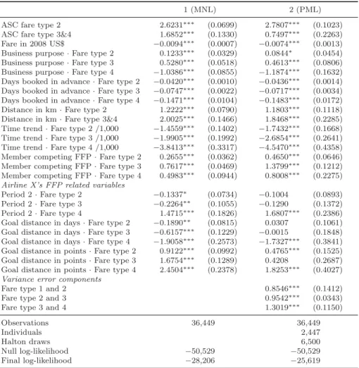
The explanatory variables are introduced in Table 2. In addition to these variables, we in-clude period and alternative specific constants to capture the non-stochastic unobserved heterogeneity amongst the four fare types. To control for general business conditions and seasonal effects, we include a trend variable. Table 3presents the estimation results as ob-tained using Biogeme (Bierlaire,2003). The standard multinomial logit model serves as a base model and ignores the implicit ordering of fare types and unobserved dependency across trips. The three error components in the panel mixed logit model show highly sig-nificant standard deviations. This indicates that implicit ordering and unobserved depen-dency matters.8 The alternative specific parameters are estimated relative to fare type 1.
The utility of buying fare type 2, for example, decreases 0.0436 every extra day the ticket is booked in advance compared with the utility of fare type 1.
Insert Table 3 about here
The estimated parameters of fare, days booked in advance, and distance have the antic-ipated sign. Booking earlier decreases the utility of buying more expensive fare types, which can be attributed to a combination of limited availability of fare types closer to departure date and business travellers booking later. People attaining more utility from more expensive fare types for longer distance flights reflects that in-flight quality is more important for long than short haul flights. The results regarding trip purpose are mixed, in particular the negative effect of a business trip on the utility of the most expensive fare type is surprising. The results show that holding multiple FFP memberships increases the probability of buying more expensive fare types.
with the goal gradient hypothesis (Taylor and Neslin,2005;Kivetz et al.,2006): the util-ity of buying more expensive fare types, hence earning more tier points, increases when getting closer to the threshold level in points. In other words, members do not fully be-have rationally and show myopic behaviour in assessing the benefits of tier tokens. We do not find such an effect for the threshold level in days. Apart from not finding the same pattern in the descriptive analysis, the unexpected signs as shown in Table 3might be at-tributed to the correlation between the two variables.
Purchase Frequency Model
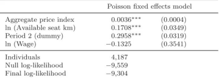
After obtaining the aggregate price index function from the panel mixed logit estimation results of the transaction size model, we estimate the purchase frequency model, as in (6), by means of a conditional fixed effects Poisson estimator.9 This estimator suffers from
overdispersion. Accounting for overdispersion, however, is fairly easy by calculating robust standard errors for which routines are available in standard software packages. Besides the aggregate price index function, we include the logarithm of income, a period dummy and the available seat kilometres as explanatory variables.
Table 4shows the results of the purchase frequency model estimation. Except for the wage effect, all estimated parameters are significant. As anticipated, an increase in the average availability of seat kilometres, due to, for example, an increased flight frequency by the airline or flying different markets by the member, has a positive effect on the de-mand for flying with airline X. While controlling for FFP effects via the transaction size model, the positive sign of the period dummy indicates that demand is higher in the pe-riod after introducing the new FFP. Hence, not taking into account this dummy variable would overestimate the impact of the new FFP on total demand.
Insert Table 4 about here
logsum, hence the denominator in the choice probability, has a positive effect on the de-mand for trips of airline X. In terms of prices, an increase in the logsum implies a decrease in the generalised price of the alternative fare types and therefore a higher expected util-ity. The price elasticity is equal to our parameter estimate, (-)0.0036, multiplied by the average value for the aggregate price index, 119US$. The price elasticity of -0.43 indicates that the demand of flying with airline X is, on average, inelastic.
We find that the income elasticity of demand is negative suggesting that people might switch to other airlines to find the fare types that match a higher income level. Examin-ing the table of fares from airline X and its main competitor, reveals that the market is vertically differentiated: the nearest variant in the price-quality space of a particular fare type might be offered by the competing airline. The income elasticity of demand, however, is not significantly different from 0. On average there seems to be only a weak link be-tween changes in income and number of flights taken with airline X. On the one hand, the precision of this estimate might improve using detailed, non aggregated income data, but on the other hand, however, we conjecture that by controlling for job, travel purpose, and other market characteristics the true income elasticity of demand for flying with airline X might be close to zero.
Effects On Usage Level Indicators
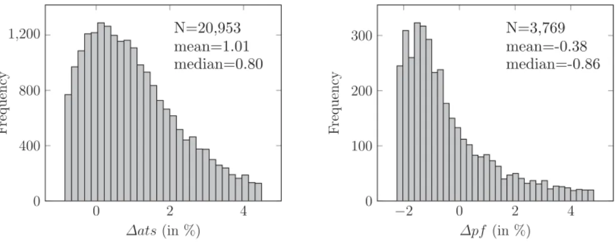
We use our estimation results to calculate the implied effect of the new FFP by comparing the average transaction size, purchase frequency, total revenues, and compensating varia-tion - as defined in equavaria-tion (7), (8), (9), and (10) - between the actual and hypothetical scenario in which the new FFP would not have been implemented. In addition to report-ing the mean and median impact per trip or member,Figure 1 andFigure 2 show the dis-tribution of the changes in each of the four measures over the sample.10 In this manner,
one can take into account that not all members necessarily react similar to (changes in) loyalty programs, as underlined by, amongst others,Dorotic et al. (2012).
Insert Figure 1 about here Insert Figure 2 about here
The left panel inFigure 1 shows that for the majority of the trips the average transaction size is higher after the implementation of the new FFP. We find that individuals on aver-age increased their averaver-age transaction size by 1 per cent to 113US$. Approximately 25 per cent of all trips yields a lower average transaction size, up to -0.85 per cent, whereas for some trips the average transaction size increased by 4.5 per cent. The right panel in
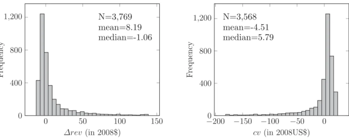
Figure 1 focusses on changes in purchase frequency. We find that the average individual has decreased the number of flights with airline X by 0.4 per cent to 4.5 trips. About 75 per cent of the light and moderate buyers flies less with airline X as a result of the new FFP. Both for the average transaction size and purchase frequency, the magnitude of the effect of the new FFP seems to be relatively small, varying between -2 and 5 per cent. The variation across members, though, is large, as one can directly observe fromFigure 1. From the firm’s perspective, the left panel of Figure 2 reveals that a small majority of individuals, 55 per cent, slightly decreased their total spending after implementing the LP design change. However, this decrease is more than compensated by the increase in spending by the other members: the total increase in revenues equals about 31,000US$ and 8.20US$ per member. Since we focus on light and moderate buyers only, our result might be the lower limit.
The right panel of Figure 2 shows the distribution of compensating variation across mem-bers. From the welfare perspective, we find a mean compensating variation of -4.53US$. As shown in the figure, however, the majority of FFP members faces a relatively small but positive compensating variation. In other words, for the majority of members the new FFP decreases well-being with a maximum of 25US$. Variation across consumers is huge;
for some members the new FFP increases well-being up until 155US$. Although the ma-jority of the FFP members is worse off, the gain in consumer surplus for the ones who are better off exceeds the losses.
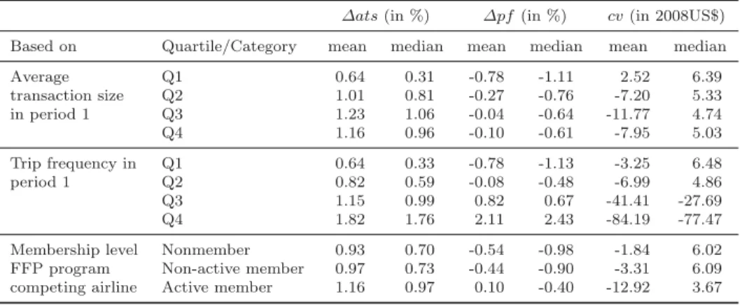
The findings clearly show that looking at the new FFP, there are winners and losers amongst airline X’s FFP members. In an effort to provide insight into the relation between mem-bers’ observed idiosyncrasies and their behavioural reactions, we show in Table 5our main results for different subgroups across the FFP members. We construct the subgroups based on average transaction size in period 1, purchase frequency in period 1, and membership tier within the competing FFP, respectively. For the first two, we define each quartile a subgroup. The leading hypothesis regarding initial usage levels and behavioural impact of loyalty programs is that light and heavy consumers do not change their behaviour due to not receiving benefits from the program or receiving them too easily while being already at the upper limit of their budget respectively, hence the most successful target group would consist of moderate buyers, see, for example,Dowling and Uncles (1997), Kivetz and Simonson (2003), Lal and Bell(2003), andLiu (2007).
Insert Table 5 about here
Looking at Table 5, we find that the purchase frequency in period 1 and the tier within the competing FFP are clear indicators for the behavioural changes of airline X’s FFP members. If members initially travel more often with airline X, they have, on average, a larger increase in the average transaction size and purchase frequency due to the new FFP. In addition, the larger negative compensating variation suggest that they also bene-fit most from the new FFP. To a lesser extent, the same holds for members that are more involved in the competing FFP. This suggests that holding multiple FFP memberships is a strong indicator for frequent fliers. The differences, however, amongst the categories, particularly for compensating variation, are smaller compared with classifying the mem-bers based on their initial purchase frequency. The picture as shown inTable 5 for
classi-fying based on average transaction size in period 1 is less clear, moderate members, pre-dominantly the third quartile, seem to be more affected by the new FFP than heavy buy-ers. In our case, average transaction size might be a bad indicator for usage levels, be-cause members who occasionally fly but buy expensive tickets are not heavy buyers, they would end up, however, in the highest quartiles based on average transaction size.
In contrast to Liu(2007), our comparison across individuals shows that light buyers in our sample are less affected by the new FFP, whereas the frequent fliers, the heavy buy-ers in our sample, do benefit most from the new FFP and change their behaviour most favourably from airline X’s perspective. The differences can be explained looking at the sample and the type of loyalty program. First, in our sample we only include light and moderate buyers, individuals who classified for the lowest tier. It is within this group that we find heavy buyers to be most affected. Second, the loyalty program we study includes tier levels as the major reward. Getting into reach to qualify for a higher tier would imply a dramatic increase in usage levels for the light buyers. Hence, they are less affected by, or even lose from the new FFP on the one hand, whereas on the other hand, the system of tier for which you need to qualify each review period keeps heavy buyers motivated to spend at airline X.
Conclusion
This article analyses the effect of loyalty programs on consumer behaviour. We use a trans-action based data set, including a 10 per cent stratified random sample of active FFP members of a particular airline. We study the behavioural impact of redesigning a fre-quency reward program into a customer tier program, accounting for self-selection and consumer heterogeneity. To do so, we set-up a quasi-natural experiment using an unantic-ipated change in the FFP design and focus only at those members who qualified for the
lowest initial tier level at the moment of change.
We model the choice of ticket type and trip frequency in a two-stage budgeting model. This model allows us to asses the impact of FFP design on consumer well being, besides the more traditional measures of LP performance, such as average transaction size, pur-chase frequency and total revenues. We estimate a combined panel mixed logit and count data model to find the parameters of interest. We find that the demand for flying with the sponsoring airline is price inelastic, but do not find evidence for an income elasticity differ-ent from 0. The average transaction size model confirm the goal gradidiffer-ent hypothesis: the utility of buying more expensive fare types increases when getting closer to a next thresh-old level in points.
We show that the inclusion of tier levels within the reward structure causes members to increase, on average, their expected transaction size by 1 per cent and to decrease their expected number of trips by 0.4 per cent. Total revenues for the sponsoring airline in-creased by 8US$ per FFP member over a 16 month period, yielding a total of 31,000US$. Over the same period, the compensating variation equals -4.5US$ per member, which im-plies that on average these members benefited from the redesigned FFP. However, we find substantial variation across individual members in their behavioural reaction. Our anal-ysis shows that individuals who benefit most from the new reward structure are those who are in the highest quartiles of flying with the sponsoring airline in the period before the change. Besides being better off, their behaviour also changes most favourably for the sponsoring airline: higher average transaction sizes, more trips and, hence, increasing rev-enues. Our findings are consistent with previous studies indicating that light buyers are less affected by loyalty programs (Dowling and Uncles,1997). Our findings, in general, confirm the commonly held belief that one should take into account observable and unob-servable consumer idiosyncrasies when evaluating loyalty programs (Liu,2007).
Bibliography
Allison, P. D. and Waterman, R. P. (2002). Fixed-Effects Negative Binomial Regression Models. Sociologi-cal Methodology, 32(1):247–265.
Banerjee, A. and Summers, L. (1987). On Frequent-Flyer Programs and Other Loyalty-Inducing Eco-nomics Arrangements.
Basso, L., Clements, M., and Ross, T. (2009). Moral Hazard and Customer Loyalty Programs. American Economic Review: Microeconomics, 1(1):101–123.
Bierlaire, M. (2003). Biogeme: A free package for the estimation of discrete choice models. InProceedings of the 3rd Swiss Transportation Research Conference, Ascona, Switzerland.
Borenstein, S. (1989). Hubs and High Fares: Dominance and Market Power in the U.S. Airline Industry.
RAND Journal of Economics, 20(3):344–365.
Breugelmans, E., Bijmolt, T. H. a., Zhang, J., Basso, L. J., Dorotic, M., Kopalle, P., Minnema, A., Mijn-lieff, W. J., and W¨underlich, N. V. (2014). Advancing research on loyalty programs: a future research agenda. Marketing Letters.
Deaton, A. and Muellbauer, J. (1980). Economics and Consumer Behavior. Cambridge University Press, Cambridge.
Dorotic, M., Bijmolt, T. H., and Verhoef, P. C. (2012). Loyalty Programmes: Current Knowledge and Research Directions.International Journal of Management Reviews, 14:217–237.
Dowling, G. R. and Uncles, M. (1997). Do Customer Loyalty Programs Really Work? Sloan Management Review, 38(4):71–82.
Gorman, W. M. (1959). Separable Utility and Aggregation. Econometrica, 27(3):469–481.
Guimaraes, P. (2008). The fixed effects negative binomial model revisited. Economics Letters, 99(1):63–66. Hausman, J. and Leibtag, E. (2007). Consumer benefits from increased competition in shopping outlets:
Measuring the effect of wal-mart. Journal of Applied Econometrics, 22:1157–1177.
Hausman, J. A., Hall, B. H., and Griliches, Z. (1984). Econometric Models for Count Data with an Ap-plication to the Patents-R&D Relationship. National Bureau of Economic Research Technical Working Paper Series, No. 17.
Hausman, J. A., Leonard, G. K., and McFadden, D. (1995). A utility-consistent, combined discrete choice and count data model Assessing recreational use losses due to natural resource damage. Journal of Public Economics, 56(1):1–30.
of Consumer Response to Loyalty Programs. Journal of Marketing Research, 40(4):454–467.
Kivetz, R., Urminsky, O., and Zheng, Y. (2006). The Goal-Gradient Hypothesis Resurrected: Purchase Acceleration, Illusionary Goal Progress, and Customer Retention. Journal of Marketing Research, 43(1):39–58.
Klemperer, P. (1987a). Markets with Consumer Switching Costs. Quarterly Journal of Economics, 102(2):375–394.
Klemperer, P. (1987b). The Competitiveness of Markets with Switching Costs. RAND Journal of Eco-nomics, 18(1):138–150.
Lal, R. and Bell, D. (2003). The impact of frequent shopper programs in grocery retailing. Quantitative Marketing and Economics, 1:179–202.
Lederman, M. (2007). Do Enhancements to Loyalty Programs Affect Demand? The Impact of Inter-national Frequent Flyer Partnerships on Domestic Airline Demand. RAND Journal of Economics, 38(4):1134–1158.
Lederman, M. (2008). Are Frequent-Flyer Programs a Cause of the Hub Premium? Journal of Economics & Management Strategy, 17(1):35–66.
Leenheer, J., van Heerde, H. J., Bijmolt, T. H. A., and Smidts, A. (2007). Do loyalty programs really enhance behavioral loyalty? An empirical analysis accounting for self-selecting members. International Journal of Research in Marketing, 24(1):31–47.
Lewis, M. (2004). The Influence of Loyalty Programs and Short-Term Promotions on Customer Retention.
Journal of Marketing Research, 41(3):281–292.
Liu, Y. (2007). The Long-Term Impact of Loyalty Programs on Consumer Purchase Behavior and Loyalty.
Journal of Marketing, 71(4):19–35.
Liu, Y. and Yang, R. (2009). Competing Loyalty Programs: Impact of Market Saturation, Market Share, and Category Expandability. Journal of Marketing, 73:93–108.
McCall, M. and Voorhees, C. (2010). The Drivers of Loyalty Program Success: An Organizing Framework and Research Agenda. Cornell Hospitality Quarterly, 51:35–52.
Morrison, S. and Winston, C. (1995). The Evolution of the Airline Industry. The Brookings Institution, Washington, D.C.
Morrison, S., Winston, C., Bailey, E., and Kahn, A. (1989). Enhancing the Performance of the Deregu-lated Air Transportation System. Brookings Papers on Economic Activity.Microeconomics, 1989:61– 123.
Rouwendal, J. and Boter, J. (2009). Assessing the value of museums with a combined discrete choice/count data model. Applied Economics, 41(11):1417–1436.
Sharp, B. and Sharp, A. (1997). Loyalty programs and their impact on repeat-purchase loyalty patterns.
International Journal of Research in Marketing, 14(5):473–486.
Strotz, R. H. (1957). The Empirical Implications of a Utility Tree. Econometrica, 25(2):269–280. Taylor, G. A. and Neslin, S. A. (2005). The current and future sales impact of a retail frequency reward
program.Journal of Retailing, 81(4):293–305.
Verhoef, P. C. (2003). Understanding the Effect of Customer Relationship Management Efforts on Cus-tomer Retention and CusCus-tomer Share Development.Journal of Marketing, 67(4):30–45.
Zhang, J. and Breugelmans, E. (2012). The Impact of an Item-Based Loyalty Program on Consumer Purchase Behavior. Journal of Marketing Research, 49:50–65.
Notes
1The proprietary data set is provided by the airline on a confidential basis, which restricts us from
nam-ing either the FFP or the airline partner.
2The initial tier level of each member has been determined by airline X based on individual usage levels
observed before launching its redesigned FFP in August 2007. Therefore, one could argue that the effect of FFPs will be overstated when including all members: any non-observable characteristics explaining differences in usage levels between members belonging to other tier levels would be erroneously attributed to the new FFP.
3We implicitly assume that decision making of consumers is myopic. Lewis(2004) points out that loyalty
programs might cause consumer behaviour to shift from myopic to dynamic decision making. Due to the afore-mentioned perfect linearly correlation, we cannot test for this latter behavioural mechanism.
4SeeRouwendal and Boter(2009) for a discussion on how to specify the model when income affects the price
index.
5This estimator does not give the individual fixed effectsμ directly. Therefore, we compute these fixed
ef-fects as the difference between the observed and the estimated total number of trips over the two periods: exp(¯μ) = (Q1+Q2)
exp(θylny1+θz1) + exp(θylny2+θz2) .
6We here only report the results of our final model specifications. We have performed sensitivity analyses
with respect to sampling and alternative specification for the transaction size model. These results are avail-able upon request. (web appendix?)
7We estimated the model with randomβ coefficients for fare and FFP effects, but then the required
num-ber of Halton draws is beyond the computational maximum to obtain robust estimates.
8Using the log-likelihood ratio test, we reject the hypothesis that the panel mixed logit model is not
bet-ter than the multinomial logit model. The test statistic,−2(LLMNL–LLP ML), equals 4,614. Hence, the null hypothesis is rejected using the critical value of 3.84.
9The conditional fixed effects negative binomial model (Hausman et al.,1984) does not eliminate time
in-variant individual specific effects from the likelihood function (Allison and Waterman,2002;Guimaraes,2008). Alternatively, we estimated the unconditional fixed effects negative binomial model. This estimator, however, suffers from incidental parameter bias.
Table 1: Number of trips per fare type, percentage in brackets.
Business Leisure
period 1 period 2 period 1 period 2
Fare type 1 (Lowest available fare) 1,147 ( 9.8) 2,113 (16.3) 1,549 (17.6) 2,589 (25.8) Fare type 2 (. . . ) 8,505 (72.5) 8,943 (69.1) 6,520 (73.9) 6,732 (67.1) Fare type 3 (. . . ) 2,033 (17.3) 1,660 (12.8) 733 ( 8.3) 587 ( 5.9) Fare type 4 (Business flexible fare) 44 ( 0.4) 217 ( 1.7) 19 ( 0.2) 125 ( 1.2)
Table 2: Mean of explanatory variables per fare type, standard deviation in brackets
Fare Days booked Distance Goal distance Goal distance Member competing in 2008US$ in advance in km in days in points FFP
Fare type 1 65.36 (14.70) 24.27 (16.59) 541 (258) 0.29 (0.32) 0.12 (0.20) 0.20 (0.40) Fare type 2 116.34 (24.87) 13.81 (13.88) 556 (266) 0.25 (0.32) 0.14 (0.24) 0.29 (0.46) Fare type 3 212.88 (37.85) 7.73 ( 9.05) 513 (217) 0.22 (0.31) 0.17 (0.27) 0.46 (0.50) Fare type 4 295.48 (90.46) 8.35 ( 9.71) 598 (349) 0.36 (0.29) 0.30 (0.28) 0.51 (0.50)
Table 3: Estimation results for transaction size model.
1 (MNL) 2 (PML)
ASC fare type 2 2.6231∗∗∗ (0.0699) 2.7807∗∗∗ (0.1023) ASC fare type 3&4 1.6852∗∗∗ (0.1330) 0.7497∗∗∗ (0.2263) Fare in 2008 US$ −0.0094∗∗∗ (0.0007) −0.0074∗∗∗ (0.0013) Business purpose·Fare type 2 0.1233∗∗∗ (0.0329) 0.0844∗ (0.0454) Business purpose·Fare type 3 0.5280∗∗∗ (0.0518) 0.4613∗∗∗ (0.0806) Business purpose·Fare type 4 −1.0386∗∗∗ (0.0855) −1.1874∗∗∗ (0.1632) Days booked in advance·Fare type 2 −0.0420∗∗∗ (0.0010) −0.0436∗∗∗ (0.0014) Days booked in advance·Fare type 3 −0.0747∗∗∗ (0.0022) −0.0717∗∗∗ (0.0034) Days booked in advance·Fare type 4 −0.1471∗∗∗ (0.0104) −0.1483∗∗∗ (0.0172) Distance in km·Fare type 2 1.2222∗∗∗ (0.0790) 1.1803∗∗∗ (0.1118) Distance in km·Fare type 3&4 2.0025∗∗∗ (0.1466) 1.8468∗∗∗ (0.2285) Time trend·Fare type 2 /1,000 −1.4559∗∗∗ (0.1402) −1.7432∗∗∗ (0.1668) Time trend·Fare type 3 /1,000 −1.9905∗∗∗ (0.1992) −2.6854∗∗∗ (0.2641) Time trend·Fare type 4 /1,000 −3.8413∗∗∗ (0.3317) −4.5470∗∗∗ (0.4358) Member competing FFP·Fare type 2 0.2655∗∗∗ (0.0362) 0.4650∗∗∗ (0.0646) Member competing FFP·Fare type 3 0.7617∗∗∗ (0.0469) 1.3799∗∗∗ (0.1212) Member competing FFP·Fare type 4 0.4983∗∗∗ (0.0944) 0.8008∗∗∗ (0.2275)
Airline X’s FFP related variables
Period 2·Fare type 2 −0.1337∗ (0.0734) −0.1004 (0.0893) Period 2·Fare type 3 −0.2264∗∗ (0.1055) −0.1290 (0.1372) Period 2·Fare type 4 1.4715∗∗∗ (0.1826) 1.6807∗∗∗ (0.2386) Goal distance in days·Fare type 2 −0.1890∗∗ (0.0815) 0.0307 (0.1061) Goal distance in days·Fare type 3 −0.6157∗∗∗ (0.1229) −0.0015 (0.1848) Goal distance in days·Fare type 4 −1.9058∗∗∗ (0.2573) −1.7327∗∗∗ (0.3841) Goal distance in points·Fare type 2 0.9122∗∗∗ (0.0992) 0.4765∗∗∗ (0.1525) Goal distance in points·Fare type 3 1.6754∗∗∗ (0.1289) 0.4208 (0.2687) Goal distance in points·Fare type 4 2.4504∗∗∗ (0.2378) 1.8253∗∗∗ (0.4027)
Variance error components
Fare type 1 and 2 0.8546∗∗∗ (0.1412) Fare type 2 and 3 0.9542∗∗∗ (0.0343) Fare type 3 and 4 1.3019∗∗∗ (0.1150)
Observations 36,449 36,449
Individuals 2,447
Halton draws 6,500
Null log-likelihood −50,529 −50,529 Final log-likelihood −28,206 −25,619 Standard errors in parentheses,∗p <0.1,∗∗p <0.05,∗∗∗p <0.01.
Table 4: Estimation results for purchase frequency model.
Poisson fixed effects model Aggregate price index 0.0036∗∗∗ (0.0004) ln (Available seat km) 0.1708∗∗∗ (0.0349) Period 2 (dummy) 0.2958∗∗∗ (0.0319) ln (Wage) −0.1325 (0.3541) Individuals 4,187 Null log-likelihood −9,559 Final log-likelihood −9,304
Table 5: Average and median implied impact of FFP accross members.
Δats(in %) Δpf(in %) cv(in 2008US$) Based on Quartile/Category mean median mean median mean median
Average Q1 0.64 0.31 -0.78 -1.11 2.52 6.39 transaction size Q2 1.01 0.81 -0.27 -0.76 -7.20 5.33 in period 1 Q3 1.23 1.06 -0.04 -0.64 -11.77 4.74 Q4 1.16 0.96 -0.10 -0.61 -7.95 5.03 Trip frequency in Q1 0.64 0.33 -0.78 -1.13 -3.25 6.48 period 1 Q2 0.82 0.59 -0.08 -0.48 -6.99 4.86 Q3 1.15 0.99 0.82 0.67 -41.41 -27.69 Q4 1.82 1.76 2.11 2.43 -84.19 -77.47
Membership level Nonmember 0.93 0.70 -0.54 -0.98 -1.84 6.02 FFP program Non-active member 0.97 0.73 -0.44 -0.90 -3.31 6.09 competing airline Active member 1.16 0.97 0.10 -0.40 -12.92 3.67
N=20,953 mean=1.01 median=0.80 0 2 4 0 400 800 1,200 Δats(in %) F requency N=3,769 mean=-0.38 median=-0.86 −2 0 2 4 0 100 200 300 Δpf (in %) F requency
N=3,769 mean=8.19 median=-1.06 0 50 100 150 0 400 800 1,200 Δrev(in 2008$) F requency N=3,568 mean=-4.51 median=5.79 −0200 −150 −100 −50 0 400 800 1,200 cv(in 2008US$) F requency
Appendix A. Definition and construction of variables
Fare We calculate the average one-way trip fare (in 2008 US$) per fare type. This aver-age fare is specific in origin-destination, days booked in advance, and departure time. We distinguish between booking< 8, 8–20, 21–60 and > 60 days in advance and departing between: 05:00–09:59, 10:00–13:59, 14:00–16:59, 17:00–20:59, and 21:00–04:59. The aver-age fare is adjusted for individual redemption behaviour using the expected value of this redemption. This value equals 0.01US$ times the number of tokens and the probability that the member uses these tokens for redemption. We approximate this probability by dividing total redeemed tokens over total accrued tokens during the three-year period.
Goal distance in days The goal distance in days is measured as the number of days passed in the annual review period divided by total number of days a year.
Goal distance in points The goal distance in points is measured as the total amount of points already accrued within the annual review period divided by the total amount of points needed to qualify for the next tier level: 20 000 for Silver and 50 000 for Gold tier.
Purpose The trip purpose is not recorded in the data. We apply a set of rules to deter-mine the purpose of trip, distinguishing between business and leisure trips, based on the available trip and FFP member data. We briefly discuss this set of rules. First, people are excluded from having a business purpose based on their job status, like for example retirees, wait staff, nurses and hairdressers. Second, if the trip departs in the morning and/or arrives in the evening peak hours on weekdays and the total trip does not include Saturday or Sunday, it is defined as a business trip. Third, trips during and including bank holidays as well as short trips starting at Friday and Saturday are labelled as leisure trips. This set of rules classifies around 95 per cent of all trips.
Wage The wage is a proxy for the income of individual members. We construct this pe-riod specific proxy using income tax return information. The reported wage and salary
income are publicly available per zip code area. We match the wage and salary income per zip code area to the place of residence of the member to approximate income.
Available seat km We calculate the available seat kilometre per origin destination pair and match this number to each observed trip in the data set. To find the final proxy, we take the average over all trips per period and per member. Therefore, the quality of a specific route gets a higher weight within the final proxy when the member travels more frequent that route.