Accelerating pseudo-marginal MCMC using Gaussian processes

This is the author’s version of a work that was submitted/accepted for pub-lication in the following source:

Drovandi, Christopher C., Moores, Matthew T., & Boys, Richard J. (2015)

Accelerating Pseudo-Marginal MCMC using Gaussian Processes.

[Working Paper] (Unpublished)

This file was downloaded from: http://eprints.qut.edu.au/90973/

c

Copyright 2015 The Author(s)

Notice: Changes introduced as a result of publishing processes such as copy-editing and formatting may not be reflected in this document. For a definitive version of this work, please refer to the published source:

Accelerating Pseudo-Marginal MCMC using Gaussian Processes

*Queensland University of Technology, Brisbane, Australia 4001 † University of Warwick, Coventry CV4 7AL, United Kingdom ‡ Newcastle University, Newcastle upon Tyne NE1 7RU, United Kingdom

email: [email protected] December 2, 2015

Abstract

Pseudo-marginal methods such as the grouped independence Metropolis-Hastings (GIMH) and Markov chain within Metropolis (MCWM) algorithms have been introduced in the liter-ature as an approach to perform Bayesian inference in latent variable models. These methods replace intractable likelihood calculations with unbiased estimates within Markov chain Monte Carlo algorithms. The GIMH method has the posterior of interest as its limiting distribution, but suffers from poor mixing if it is too computationally intensive to obtain high-precision likelihood estimates. The MCWM algorithm has better mixing properties, but less theoret-ical support. In this paper we propose to use Gaussian processes (GP) to accelerate the GIMH method, whilst using a short pilot run of MCWM to train the GP. Our new method, GP-GIMH, is illustrated on simulated data from a stochastic volatility and a gene network model.

Keywords: Gaussian processes, likelihood-free methods, Markov processes, particle Markov

1

Introduction

Bayesian inference on high-dimensional latent variable models is currently challenging. The mixing of Markov chain Monte Carlo (MCMC) samplers can be poor when there is correlation between the parameter of interest and the latent variables. Pseudo-marginal methods have been introduced by Beaumont (2003) and Andrieu and Roberts (2009) as an approach to improve the statistical efficiency of MCMC. Pseudo-marginal methods work by replacing the actual likelihood with an unbiased likelihood estimator in the Metropolis-Hastings ratio. It is possible then to make proposals for the Markov chain directly on the space of the parameter of interest, rather than conditional on the value of a set of the latent variables.

One of the pseudo-marginal methods is referred to as the grouped independence Metropolis-Hastings (GIMH) method in Beaumont (2003). In the GIMH approach, the likelihood esti-mate for the current value of the chain is recycled to the next iteration. Andrieu and Roberts (2009) show that the GIMH method has the desired posterior as its limiting distribution. The drawback of the GIMH method is that it may suffer from poor mixing if the likelihood is not estimated with high precision. The major issue is that the Markov chain can become stuck if the likelihood is grossly overestimated. For complex applications it may be too expensive to obtain likelihood estimators with low variance. However, given the “exact-approximate” na-ture of GIMH, in the sense that the method is exact up to Monte Carlo error despite using an approximate likelihood, it has received considerable attention in the literature (e.g. Andrieu et al. (2010) and Doucet et al. (2015)).

The other pseudo-marginal method, the Markov chain within Metropolis (MCWM, Beaumont (2003)) algorithm, estimates the likelihood at both the current and proposed values of the Markov chain at every iteration. The MCWM method generally possesses better mixing properties as it able to escape an overestimated likelihood value by re-estimating it at the next MCMC iteration. However, the MCWM method does not have the posterior distribution of the parameter of interest as its limiting distribution. Because of this lack of theoretical support, MCWM has received comparatively less attention.

In this paper we make use of a Gaussian process (GP) to accelerate the GIMH method while at the same time accepting some approximation to the posterior distribution of interest. GPs have been used for the emulation of complex, deterministic models by Kennedy and O’Hagan (2000, 2001). Conrad et al. (2015) use local polynomials or GPs in a Metropolis-Hastings algorithm to reduce the number of model evaluations that are required. However, the focus of Conrad et al. (2015) is not on applications where a stochastic likelihood estimator is available. Wilkinson (2014) proposed that GPs be used to accelerate approximate Bayesian computation (ABC) methods, where the likelihood is approximated by generating many model simulations from each proposed parameter value, and measuring the distance between observed and simu-lated data through a careful choice of summary statistics. This approach uses GPs to emulate the actual log-likelihood surface based on noisy estimates obtained through simulation. The method iteratively uses the GP to discard implausible parts of the parameter space, re-trains the GP in the updated not-implausible part of the parameter space and continues this pro-cess until the GP fit has been deemed as satisfactory. The final GP is then used within an MCMC method to predict the log-likelihood surface at all proposed values of the parameter of interest.

We follow a similar approach to accelerate pseudo-marginal methods. However, one key difference is that we take advantage of the pseudo-marginal literature. In particular, we use a short run of the MCWM method as a natural approach to obtain training samples for the GP in non-negligible regions of the posterior support. The MCWM method is ideal for training the GP due to its useful mixing property and our experience with the approach is that it is generally conservative, allowing the tails of the posterior to be explored. The fitted GP is used to replace expensive likelihood estimations within the GIMH method.

Tran et al. (2015) develop a variational Bayes approach that can be used in any applica-tion where an unbiased likelihood estimator is available to approximate the posterior more efficiently compared to GIMH. However, the variational approximation is typically of a para-metric form and assumptions are sometimes made that the parameters are independent a posteriori.

Rasmussen (2003) use GPs to accelerate the Hamiltonian Monte Carlo (HMC) method for Bayesian inference when posterior density evaluation is expensive. The proposal distribution in HMC involves approximately solving a Hamiltonian system, which requires several evalu-ations of the posterior distribution. Rasmussen (2003) use a GP trained from a pilot HMC run to approximate posterior evaluations required in the HMC proposal. The method of Ras-mussen (2003) remains exact as the GP is used only for the proposal and a Metropolis-Hastings (MH) correction is applied to account for the fact that the Hamiltonian is only solved approx-imately. The MH correction step requires an evaluation of the (expensive) exact posterior density.

A related literature is on the delayed acceptance MCMC method (Christen and Fox, 2005). In delayed-acceptance MCMC, each proposed parameter goes through an initial Metropolis-Hastings step where the actual posterior density is replaced by a computationally cheap pos-terior approximation. The idea of the method is that ‘poor’ proposals can be rejected quickly and the majority of ‘promising’ proposals make it through to the next Metropolis-Hastings stage, which involves exact posterior density evaluations. The second Metropolis-Hastings step is constructed so that the Markov chain has the correct limiting distribution. As an example, Golightly et al. (2015) perform Bayesian inference for Markov jump processes us-ing the correspondus-ing linear noise approximation in the screenus-ing Metropolis-Hastus-ings step. Sherlock et al. (2015) consider a more general approach and use aknearest neighbour surro-gate within a delayed-acceptance MCMC algorithm when the likelihood is expensive or when the likelihood is estimated unbiasedly. Although the delayed-acceptance MCMC approach is exact, Golightly et al. (2015) and Sherlock et al. (2015) report efficiency gains of generally less than an order of magnitude. Our motivation here is to obtain significant speed-ups in very complex applications whilst accepting some approximation to the posterior.

The paper has the following outline. In Sections 2 and 3 we provide a brief overview of pseudo-marginal methods and GPs, respectively. In Section 4 we present our new method, GP-GIMH, which uses the MCWM algorithm to train the GP and subsequently uses the GP to accelerate the GIMH method. Finally, in Section 6, we conclude with a discussion on practicalities and potential future work.

2

Pseudo-Marginal MCMC

Suppose we have observed datay∈Ywhich is described by a statistical model with likelihood function p(y|θ) and depends on an unknown parameter θ ⊆ Rp. Prior beliefs about the parameter are summarised by the prior densityp(θ). We assume that the model requires, or is facilitated by, an auxiliary variable x ∈ X, whose value is not of direct interest. In this scenario the complete data likelihood isp(y,x|θ) =p(y|x,θ)p(x|θ) and leads to the observed data likelihood

p(y|θ) =

Z

X

p(y|x,θ)p(x|θ)dx.

Ideally this observed data likelihood is combined with the prior to make inferences about the parameters via the posterior densityp(θ|y)∝p(θ)p(y|θ). However, in non-toy problems the observed data likelihood is an analytically intractable integral. Therefore the parameter posterior is accessed as the marginal of the joint posterior for all unknowns, that is, via

p(θ|y) =

Z

X

p(θ,x|y)dx.

A standard Bayesian approach for fitting such a latent variable model is to develop an MCMC algorithm that samples the joint posteriorp(θ,x|y) and marginalises by ignoring the x sam-ples. A common approach is to develop an MCMC algorithm using two blocks,θ andx, that iteratively samples from the full conditionals p(θ|x,y) and p(x|θ,y). A key problem with such algorithms is that they can mix poorly because of high posterior correlation between the blocksθ and x. In an attempt to overcome the mixing issue, Beaumont (2003) develop algorithms that replace the computationally intractable likelihood p(y|θ) with an unbiased estimate ˆp(y|θ). The underpinning mathematics of these pseudo-marginal MCMC algorithms is studied in Andrieu and Roberts (2009) and they develop conditions under which they in-deed have the correct posterior distributionp(θ,x|y) as their limiting distribution. A simple example of an unbiased likelihood estimate is one obtained through importance sampling, namely ˆ p(y|θ) = 1 N N X i=1 p(y|xi,θ)p(xi|θ) q(xi) , wherex1, . . . ,xN iid

∼q(x) andqis an importance density defined onX. Alternative approaches to obtaining an unbiased likelihood estimate are available. For example, Andrieu et al. (2010) show that when the model of interest is a state-space model, the likelihood p(y|θ) can be estimated unbiasedly using a particle filter. Such pseudo-marginal methods are referred to as particle Markov chain Monte Carlo (PMCMC); here the term ‘particle’ denotes the use of a particle filter in obtaining the unbiased likelihood estimate. The motivation behind pseudo-marginal methods is to facilitate the proposal of new values ofθ in the Markov chain independently of latent statex. We consider a state-space model example in Section 5. Beaumont (2003) develop two algorithms. The first, referred to as grouped independence Metropolis-Hastings (GIMH), is shown in Algorithm 1. The GIMH algorithm is effectively

Algorithm 1GIMH algorithm of Beaumont (2003). Input: θ0 and iters

Output: MCMC output θ1, . . . ,θiters 1: Compute φ0 = ˆp(y|θ0₎ 2: for i= 1 toitersdo 3: Proposeθ∗ ∼q(·|θi−1) 4: Compute φ∗ = ˆp(y|θ∗) 5: Compute α= min n 1,_φi−φ1∗_pp₍(_θθi∗−)q1(₎θ_qi₍−_θ1∗|_|θ_θ∗i−)1₎ o 6: Draw u∼ U(0,1) 7: if u < αthen 8: Setφi =φ∗ and θi=θ∗ 9: else 10: Setφi _=φi−1 _{and θ}i _=θi−1 11: end if 12: end for

a standard Metropolis-Hastings algorithm in which the intractable likelihood at a new pro-posalθ∗is replaced by an unbiased likelihood estimate. Note that the likelihood at the current valueθ is not re-estimated but simply recycled from the previous iteration.

Andrieu and Roberts (2009) show that the GIMH algorithm has the posterior p(θ|y) as its limiting distribution. If we denote all the random numbers used to produce an unbiased likelihood estimate asηand considering a target posterior distribution on the extended space of (θ,η), theθ marginal target of interest is proportional top(θ)E[p(y|θ,η)] wherep(y|θ,η) is the likelihood estimate given the random numbers and the expectation is taken with respect to the distribution ofηgiven θ. The unbiased nature of the likelihood estimator implies that the expectation is p(y|θ) giving the desired posterior distribution as the target. Given this theoretically appealing property, the GIMH method has been more prominent in the literature (e.g. Andrieu et al. (2010), Doucet et al. (2015) and Sherlock et al. (2015)) compared to the other approach developed in Beaumont (2003), the Monte Carlo within Metropolis (MCWM) algorithm. However, the GIMH method can get stuck when the likelihood is substantially overestimated at any given iteration. Doucet et al. (2015) suggest that for good performance in the GIMH algorithm, the log-likelihood should be estimated with a standard deviation of roughly 1. However, in complex applications, it may be computationally difficult to achieve this goal.

The second algorithm of Beaumont (2003) (MCWM) is the same as GIMH except for the extra step where the likelihood at the current θ is re-estimated and not recycled from the previous iteration; see Algorithm 2. Although MCWM requires roughly double the amount of computational effort per iteration relative to GIMH, it does not suffer from stickiness in the Markov chain. However, the drawback is that the limiting distribution of MCWM is only the posteriorp(θ|y) in the limit asN → ∞. In our experience, MCWM produces an approximate posterior that is less precise than the actual posterior for finiteN, and thus could be considered a conservative method in the sense that the posterior variances are overestimated.

log-Algorithm 2MCWM algorithm of Beaumont (2003). Input: θ0 and iters

Output: MCMC output θ1, . . . ,θiters 1: Compute φ0 = ˆp(y|θ0₎ 2: for i= 1 toitersdo 3: Compute φi = ˆp(y|θi) 4: Proposeθ∗ ∼q(·|θi−1₎ 5: Compute φ∗ = ˆp(y|θ∗) 6: Compute α= minn1, φ∗p(θ∗)q(θi−1|θ∗) φi−1_p(θi−1_)q(θ∗_| θi−1) o 7: Draw u∼ U(0,1) 8: if u < αthen 9: Setθi =θ∗ 10: else 11: Setθi =θi−1 12: end if 13: end for

likelihood surface as a function ofθ with a GP, where the GP is trained in relevant parts of the parameter space based on the output of a short run of MCWM.

3

Gaussian Processes

Gaussian processes can be used as a prior distribution to describe uncertainty about an unknown function f(·). They are characterised by a mean function mβ(θ) and covariance function Cγ(θ,θ0) = cov{f(θ), f(θ0)}, where β and γ are so-called hyperparameters of the GP. A Gaussian process has the property that the joint distribution for the values of the function at a finite collection of points has a multivariate normal distribution; see, for example, Rasmussen and Williams (2006). In this paper, the function we wish to emulate is the log-likelihood function f(θ) = logp(y|θ). We assume a GP prior with a mean function that is quadratic in the parameter components

mβ(θ) =β0+ p X k=1 βkθk+ p X `≥k=1 βk`θkθ`,

whereθkis thekth component of the parameter vectorθandβ= (β0, β1, . . . , βp, β11, . . . , βpp)>. To assist us in selecting the covariance function, we assume that the log-likelihood surface is smooth. A suitable covariance function to uphold that assumption is the squared exponential function, which is infinitely differentiable and thus imposes a strong prior assumption that the output of the Gaussian process is very smooth. We consider the automatic relevance de-termination version of the squared exponential covariance function (Rasmussen and Williams, 2006, pp. 106), which has the form

Cγ(θ,θ0) =hcexp ( −1 2 p X k=1 (θk−θk0)2 r_k2 ) ,

whereγ= (hc, r1, . . . , rp)>.

We can estimate the GP hyperparameter ξ = (β,γ, h) using a training sample containing evaluations of the log-likelihood at a set ofJ (input) values Θ = (θ1, . . . ,θJ). We denote this training sample by DT = {θj,fˆ(θj)}Jj=1. These function evaluations are only estimates of

the log-likelihood and so we need to model their sampling distribution. We assume that the estimates are unbiased and are normally distributed with varianceh. This assumption is not quite correct as the estimates of the log-likelihood are not exactly unbiased and there may be some small dependence of their accuracy on the input θ. Nevertheless we believe that this description captures the key aspects of the sampling distribution and has the great benefit of simplifying the form of GP prediction. Specifically, taking account of the variability in the function evaluations requires that we add a nugget term to the covariance function, so that

cov{fˆ(θ),fˆ(θ0)}=Cγ(θ,θ0) +h1(θ=θ0),

where1(·) denotes the indicator function, which is 1 if its argument is true and 0 otherwise. Denote theJ×1 vectors of log-likelihood estimates and (prior) mean functions as f(Θ) and

mβ(Θ), where f(Θ)j = ˆf(θj) and mβ(Θ)j = mβ(θj), and the J ×J covariance matrix derived from the covariance function asCγ(Θ,Θ) whereCγ(Θ,Θ)ij =Cγ(θi,θj). Under the GP model assumption, we have thatf(Θ)∼ N {mβ(Θ), Cγ(Θ,Θ) +hI}, whereI is theJ×J identity matrix. This result is obtained by integrating over the random variables describing the actual function values at the training input values and is thus often referred to as the marginal likelihood. The hyperparameter can therefore be estimated via maximising the log marginal likelihood, that is, taking

ˆ ξ= arg min ξ {f(Θ)−mβ(Θ)}>{Cγ(Θ,Θ) +hI}−1{f(Θ)−mβ(Θ)}+ log|Cγ(Θ,Θ) +hI| . (1) In practice the estimate is obtained using a numerical scheme and so we use multiple starting values for the optimisation process in order to obtain a result that we believe to be close to the maximum (marginal) likelihood estimate.

The fitted GP is the posterior distribution of the log-likelihood function in light of the observed training data. It can be used to predict the value of the log-likelihood functionf(θ) at any valueθ as its posterior distribution isf(θ)|DT ∼ N {m∗(θ), s∗(θ)2}, where

m∗(θ) =m_βˆ(θ) +Cγˆ(Θ,θ)>{Cγˆ(Θ,Θ) + ˆhI}−1{f(Θ)−m_βˆ(Θ)}, (2)

s∗(θ)2=Cγˆ(θ,θ)−Cˆγ(Θ,θ)>{Cˆγ(Θ,Θ) + ˆhI}−1Cγˆ(Θ,θ), (3)

and Cγˆ(Θ,θ) is a J ×1 vector, with Cγˆ(Θ,θ)j = Cγˆ(θj,θ). Note that the variance term does not include the nugget as we want to predict the log-likelihood itself and not a noisy estimate. It is also important to note that the computational complexity of the GP prediction isO(J3). If the hyperparameter estimate ˆξand the training dataD_T are static then the inverse computation{Cγˆ(Θ,Θ)+ˆhI}−1can be re-used for each newθ. However, if additional training

data is added then the inverse must be re-computed. In such cases it is of interest to limit the value ofJ.

4

Pseudo-Marginal MCMC using Gaussian Processes

Our main objective is to mimic the process of the GIMH algorithm. However, we also wish to overcome the limitations of GIMH, namely, its computational expense and poor mixing properties for complex models. To do this we propose to use GPs to emulate the underlying unobserved log-likelihood function of the observed data. Our approach in full can be found in Algorithm 3. We refer to our new algorithm as GP-GIMH. Below we provide more detail about each of the steps.

Firstly, the GP needs to be trained. It is not feasible to train the GP over the entire param-eter space Θ⊆Rp. Here we suggest using the observed data to help identify an appropriate training region and also the values ofθ within the training region. We do this by performing a short run of MCWM and recording the parameter value and estimated log-likelihood values encountered during the algorithm. Note that, by the nature of the MCWM algorithm, two estimated log-likelihood values are generated at each iteration and we include all this infor-mation (even those from rejected proposals in the MCWM algorithm) in the training sample. Our motivation for using MCWM to determine the training sample for the GP is three-fold: (i) it harnesses the observed data and thus most of the training points will be parameter values with non-negligible posterior density; (ii) it has good mixing properties ensuring that the GP is trained at a wide range of plausibleθ values; and (iii) the MCWM method is conservative and so it can provide good coverage of the tails of the posterior distribution. However, since MCWM is conservative, it may visit parameter regions where the log-posterior is very low (especially for proposals rejected by the algorithm) and so we suggest removing points with very low log-posterior values from the training sample so that the GP can focus its training on plausible regions of parameter space.

The rest of the GP-GIMH algorithm proceeds in a similar manner to the standard GIMH method but, because our GP prediction of the log-likelihood at a proposed valueθ∗isf(θ∗)∼ N {m∗(θ∗), s∗(θ∗)2}, we simulate a likelihood estimate from a log-normalLN {m∗(θ∗), s∗(θ∗)2}

distribution. This likelihood estimate at the current parameter is recycled to the next itera-tion. Care must be taken ifs∗(θ∗) is large as this implies that the GP is not accurate atθ∗. Therefore we introduce into the algorithm an accuracy parameterwhich declares a GP pre-diction as not trustworthy whens∗(θ∗) > . Note that we only check this condition if θ∗ is accepted; this ensures that it is not necessary to have an accurate GP prediction in the tails of the posterior where parameter values are likely to be rejected. However, ifθ∗ is accepted

when s∗(θ∗) > then we suggest it is necessary to obtain a more accurate GP prediction

to check if θ∗ was wrongly accepted. In this situation we obtain K independent estimates of f(θ∗) = logp(y|θ∗) and determine their mean. Under our normality assumption of the log-likelihood estimates, this mean also has a normal distribution: ¯fK(θ∗)∼ N {f(θ∗),ˆh/K}. We can incorporate this information into our beliefs about the log-likelihood at this point using a simple Bayes update, to give

f(θ∗)|DT,f¯K(θ∗)∼ N m∗(θ∗)/s∗(θ∗)2+Kf¯K(θ∗)/ˆh 1/s∗(θ∗)2_+K/hˆ , 1 1/s∗(θ∗)2_+K/ˆ_h ! . (4)

Therefore the number of additional independent log-likelihood estimates needed to secure a sufficiently accurate GP prediction isK =dhˆ{−2 −s∗(θ∗)−2}e. If these multiple estimates

can be farmed out across sayA available processors then the number of batches of estimates to achieve this goal isdK/Ae. We allow a burn-in phase consisting ofB iterations where such additional likelihood estimates can be appended to the training sample D_T. The motivation for this burn-in phase is to assist the GP in being trained in important regions not explored sufficiently in the MCWM phase. We find in Section 5 that the burn-in phase is useful in applications where it is very expensive to estimate the likelihood. The computational draw-back of the burn-in phase is that the matrix inversion in (2) and (3) must be re-computed. However, in demanding applications these additional matrix inversions can be relatively neg-ligible. We allow for an optional step where the GP hyperparameter is re-estimated after the burn-in phase. We note that the relative computing time for this should be short in complex applications as the current hyperparameter estimate can be used as a starting value.

It might be tempting to continually grow the training sample through the entire algorithm and thereby obtain a more accurate GP across more of the parameter space. However, not only would this require additional time-consuming calculations of matrix inverses (of increasing size) but we also find that, as this alters the GP fit in areas previously explored, it creates unusual trace plots; essentially the target distribution of the algorithm is changing. We discuss this in more detail in Section 6. Once the additional training data at θ∗ is obtained we perform another Metropolis-Hastings accept/reject step but where the log-likelihood estimate is simulated based on (4).

The value of controls the level of uncertainty allowed of the GP model when parameter values are accepted. If is set too large then a parameter value may be accepted with a grossly overestimated log-likelihood value and lead to stickiness in the Markov chain, similar behaviour that can be observed in the standard GIMH method. Recall that Doucet et al. (2015) suggest that the log-likelihood should be estimated with a standard deviation of roughly one for the GIMH method to have similar statistical efficiency to a standard Metropolis-Hastings method where the likelihood is available. For our examples we find that <2 is a suitable choice.

In practice we choose by performing some very short pilot runs and ensuring that for the majority of acceptedθ∗ we have s∗(θ∗)> . Some insight into a suitable value of may also be obtained by inspecting the empirical distribution of the GP prediction standard deviations at the training points{s∗(θj), θj ∈ DT}. Ifis not in the upper tail of this distribution then this indicates that the GP training set DT requires additional training points as otherwise many additional log-likelihood estimates will be needed in GP-GIMH and little algorithmic speed-up will be obtained.

The speed-up of the GP-GIMH approach is roughlyT /(2ρT +G) where T is the time taken to run GIMH forQ iterations, 2ρT is the time for the MCWM pre-computation step where

ρ = L/Q and the value of 2 denotes the fact that two likelihood estimations are required at each iteration of MCWM, and G is the remaining time of the GP-GIMH method. In this paper we assume thatT is very large; it is computationally demanding to estimate the likelihood. In such cases G may be negligible in comparison, in which case the speed-up is roughly Q/(2L). Thus it is of interest to set L small. However, if L is set too small then G

may become non-negligible since the GP may be too uncertain across much of the parameter space. Furthermore we note thatLwill naturally need to increase as the parameter dimension grows (although it may be of interest to increaseQ as well). The value of G will also likely

increase with the parameter dimension since it becomes increasingly difficult to train the GP in areas of non-negligible posterior support. In summary, the GP-GIMH approach does suffer from the curse of dimensionality. Nonetheless, in Section 5, we demonstrate that it is possible to achieve significant speed-ups on non-trivial models of moderate dimension. It is important to note that the above discussion only considers the computational gains. We generally find an improved acceptance rate with GP-GIMH over GIMH, adding to the overall efficiency gains of GP-GIMH.

Our approach uses the MCWM algorithm to train the GP whereas Wilkinson (2014) use a history matching approach, which iteratively fits a GP to samples drawn from a hypercube, which shrinks upon each successive GP fit. This process may be expensive in moderate dimensions if uninformative priors are used and it does not exploit the correlation between parameters as our approach does. Our remaining MCMC algorithm that uses GP predictions is similar to Wilkinson (2014). However, we include the novel aspects of obtaining additional likelihood estimates when required and a burn-in phase.

All computations involving GPs are facilitated by thegpml package (Rasmussen and Williams, 2006) in MATLAB, particularly the functionsminimize and gp. The functionminimize runs the optimisation process to estimate the hyperparameter. The functiongp returns the mean and variance of the GP prediction with and without the nugget. However, we note that in (2) and (3), information regarding the expensive matrix inversion can be pre-stored as the training sample is static for all iterations in GP-GIMH after the burn-in phase. Further, the

gp function contains extensive error checking and additional unnecessary computations for our purposes. Thus we implement our own function, based on gp, to obtain the mean and variance of the GP prediction. We find that GP-GIMH based on our GP prediction code runs roughly two to three times faster compared to the version that usesgp.

5

Examples

5.1 Stochastic Volatility Example 5.1.1 Model and Data

We illustrate our method by analysing data simulated from a stochastic volatility model in Chopin et al. (2013); this paper (and some of the references therein) give more details of the model construction and its interpretation. The observation at time t is scalar and has distribution yt ∼ N(µ+βvt, vt), where vt denotes the evolving and unobserved variance of the observation process. Here µ and β are static parameters. The evolution of the state of the process follows

vt= 1 λ  zt−1−zt+ k X j=1 fj  , wherek∼ Po(λξ2/w2),c1:k iid ∼ U(t−1, t),f1:k iid ∼ Exp(ξ/w2), andzt=e−λzt−1+Pkj=1e−λ(t−cj)fj, and Po, U and Exp denote the Poisson, uniform and exponential distributions respectively. Here w2, ξ and λ are additional static parameters so that the full parameter set is θ =

Algorithm 3GP-GIMH algorithm.

Input: θ0, threshold , burn-inB and iters Output: MCMC output θ1, . . . ,θiters

1: Perform an MCWM algorithm for (a relatively small) L iterations to help determine an initial training sample. All of the information from the MCWM should be kept, including that from rejected samples. If L is too large for fast GP prediction, then the output of MCWM can be thinned to a desired level. Discard from the training set any relatively low log-likelihood estimates. The training sample after these processes is denoted as

D_T ={θ_j,fˆ(θj)}Jj=1

2: Estimate the hyperparameter ξ= (β,γ, h) of the GP using the training sampleDT

3: Simulate φ0 ∼ LN {m∗(θ0), s∗(θ0)2} from the fitted GP. θ0 can be chosen based on the MCWM pilot run

4: for i= 1 toitersdo

5: Proposeθ∗ ∼q(·|θi−1)

6: Simulateφ∗ ∼ LN {m∗(θ∗), s∗(θ∗)2} from the fitted GP

7: Compute α= min n 1, φ∗p(θ∗)q(θi−1|θ∗) φi−1_p(θi−1_)q(θ∗_|θi−1₎ o 8: Draw u∼ U(0,1) 9: if u < αthen 10: if s∗(θ∗)≤ then 11: Set φi =φ∗ andθi =θ∗ 12: else

13: Obtain dK/Ae batches of K independent likelihood estimates and update m∗(θ∗) and s∗(θ∗) using (4)

14: Ifi≤bthen append the likelihood estimates to the training sampleD_T. Optional: If i = B then re-estimate the hyperparameter ξ based on the updated training sample DT

15: Simulate φ∗ ∼ LN(m∗(θ∗), s∗(θ∗)2) from the fitted GP

16: Compute α= min n 1,_φi−φ1∗_pp₍(_θθi∗−)q1(₎θ_qi₍−_θ∗1|_|θ_θ∗i−)1₎ o 17: Draw u∼ U(0,1) 18: if u < αthen 19: Setφi=φ∗ and θi =θ∗ 20: else 21: Setφi=φi−1 and θi=θi−1 22: end if 23: end if 24: else 25: Setφi =φi−1 and θi =θi−1 26: end if 27: end for

0 1000 2000 3000 4000 5000 −4 −2 0 2 4 t y

Figure 1: Data simulated from the stochastic volatility model of Section 5.1.1.

µ, β ∼ N(0,2) and λ∼ Exp(1). Also we initialise thez-process using z0 ∼ Ga(ξ2/w2, ξ/w2),

whereGa(a, b) denotes the gamma distribution with meana/b.

The observed data for this example has been generated from the model using the same pa-rameter values as in Chopin et al. (2013), namely w2 = 0.0625, µ = 0, ξ = 0.25, β = 0 and

λ= 0.01. However, our data are a longer series with 5000 observations (as opposed to their 1000 observations). The length of our time series creates a challenging problem for PMCMC algorithms. The data are shown in Figure 1.

5.1.2 Implementation Details

Unbiased likelihood estimates are determined by using the bootstrap particle filter of Gordon et al. (1993) withN = 800 particles. This value ofN produces an estimated log-likelihood with a standard deviation of roughly 2.5 at the true parameter value. For the GIMH method, we also considerN = 500 andN = 1000 so that an essentially un-optimised GP-GIMH approach is compared to a close-to-optimal GIMH run. To further improve the performance of GIMH, we use the multiple-core PMCMC approach of Drovandi (2014) which uses multiple cores (here A= 16 cores) to obtain independent likelihood estimates for each proposed parameter value and takes the average in order to reduce the variance of the estimated likelihood. We run 100K iterations of GIMH. We also consider MCWM with N = 800 but only run it for 50K iterations as this algorithm requires two likelihood estimates at each iteration. We use the 16 cores in a similar way to improve the accuracy of MCWM.

For the MCWM pre-computation step of GP-GIMH we use L= 1500. During this step, we adapt the covariance matrix of the multivariate normal random walk proposal every 10th iter-ation, following an initial 50 iterations. Recall that this MCWM output is only used to train the GP. We do not take advantage of any parallel computing in the MCWM pre-computation phase to illustrate that the GP-GIMH can be effective even when the likelihood is not esti-mated as precisely as in our implementations of the standard GIMH and MCWM methods.

The maximum log-posterior estimate encountered during the MCWM pre-computation phase is roughly−4610. We discard any log-posterior estimates below −4705. To investigate the effect of the training sample size, J, we use all samples obtained from the MCWM pre-computing step and also thin the output by a factor of 2, producing (roughly)J = 1500 and

J = 3000. For comparison purposes the remaining part of GP-GIMH (again 100K iterations) uses the same multivariate normal random walk as GIMH/MCWM. No burn-in phase is used for GP-GIMH (i.e. no additional log-likelihood estimates are added to the training sample). We considervalues of 1, 1.5 and 2. When the tolerance condition is not met, we obtain in-dependent likelihood estimates (at the proposed parameter) in batches of sizedK/Ae, where

A = 16. We also make the 16 cores available in the the remaining part of the GP-GIMH algorithm as MATLAB automatically parallelises some of the computations. We run the full GP-GIMH procedure independently five times for each combination ofJ and .

To simplify comparisons between methods, we assume that a suitable starting value and mul-tivariate normal random walk covariance matrix have already been determined, which are used for each algorithm (except the MCWM pre-computing phase, which adaptively deter-mines a covariance matrix). Here we use the true parameter value to initialise the chain and an updating matrix obtained from some pilot runs. We note that, in reality, it is likely that the GP-GIMH algorithm would be faster at determining a suitable covariance matrix given that pilot runs can be performed quickly. This could also be a strong motivation for using a GP-GIMH algorithm if exact inferences are necessary (up to Monte Carlo error). We now explore the accuracy of the GP-GIMH algorithm in determining the posterior distribution.

5.1.3 Results

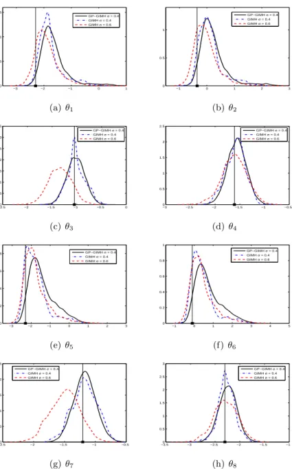
We find the marginal posterior estimates of GP-GIMH are insensitive to the choices of

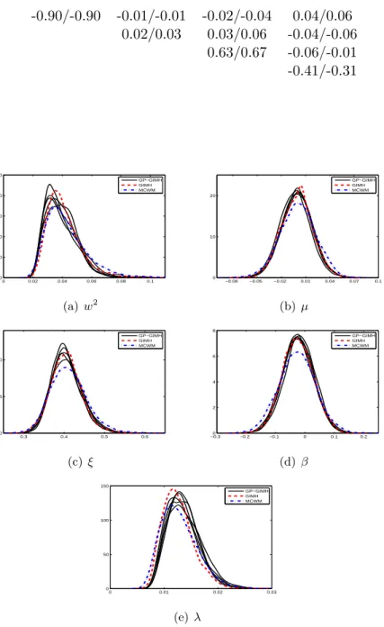
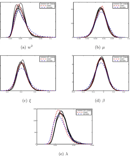
(see Appendix A). Very occasionally there is a distortion in the posterior tail when = 2.0. Given the insensitivity to , in Figures 2 (J ≈ 1500) and 3 (J ≈ 3000) we only present results for = 1. Shown in the figures are results from the 5 independent runs of GP-GIMH, as well as the results produced by GIMH and MCWM. It is evident that GP-GIMH is able to produce quite accurate estimates of the marginals, competitive with and sometimes better than MCWM. However, the GP-GIMH algorithm has more difficulty approximating the posterior distributions that show some skewness. One drawback of GP-GIMH is there is some between-run variability, which is more apparent for the posterior distributions that deviate away from symmetry. It is likely that this variability comes from different GP fits resulting from different MCWM pre-computing runs. From Figure 3 it is evident that the between run variability is reduced slightly when using the larger training sample size,J ≈3000.

Table 1 shows the upper triangular part of the estimated posterior correlation matrix from a run of GIMH and one of the runs of GP-GIMH. It is evident that GP-GIMH is able to produce reasonable estimates of the posterior correlation matrix in this example, and confirming that the algorithm could be useful for determining a suitable proposal distribution for GIMH. Table 2 shows the run times (averaged over the 5 independent runs) for GP-GIMH (excluding the MCWM pre-computing phase and GP fitting) for different combinations of J and . Interestingly there is little sensitivity to the run times with respect to . Intuitively, the run time should decrease with an increase in . We suggest that for proposals with s∗(θ∗) >

Table 1: Upper triangular part of the posterior correlation matrix for θ obtained from the GIMH/GP-GIMH (first run withJ ≈1500 and= 1.0) algorithms for the stochastic volatility model. -0.90/-0.90 -0.01/-0.01 -0.02/-0.04 0.04/0.06 0.02/0.03 0.03/0.06 -0.04/-0.06 0.63/0.67 -0.06/-0.01 -0.41/-0.31 0 0.02 0.04 0.06 0.08 0.1 0 10 20 30 40 50 GP−GIMH GIMH MCWM (a) w2 −0.08 −0.05 −0.02 0.01 0.04 0.07 0.1 0 10 20 GP−GIMH GIMH MCWM (b)µ 0.3 0.4 0.5 0.6 0 5 10 GP−GIMH GIMH MCWM (c)ξ −0.30 −0.2 −0.1 0 0.1 0.2 2 4 6 8 GP−GIMH GIMH MCWM (d)β 0 0.01 0.02 0.03 0 50 100 150 GP−GIMH GIMH MCWM (e)λ

Figure 2: Estimated marginal posterior densities for the stochastic volatility example from runs of the GIMH (red dash) and MCWM (blue dash-dot) algorithms and five independent runs of the GP-GIMH (black solid) algorithm withJ ≈1500 and= 1.

0 0.02 0.04 0.06 0.08 0.1 0 10 20 30 40 GP−GIMH GIMH MCWM (a) w2 −0.08 −0.05 −0.02 0.01 0.04 0.07 0.1 0 10 20 GP−GIMH GIMH MCWM (b)µ 0.3 0.4 0.5 0.6 0 5 10 GP−GIMH GIMH MCWM (c)ξ −0.30 −0.2 −0.1 0 0.1 0.2 2 4 6 8 GP−GIMH GIMH MCWM (d)β 0 0.01 0.02 0.03 0 50 100 150 GP−GIMH GIMH MCWM (e)λ

Figure 3: Estimated marginal posterior densities for the stochastic volatility example from runs of the GIMH (red dash) and MCWM (blue dash-dot) algorithms and five independent runs of the GP-GIMH (black solid) algorithm withJ ≈3000 and= 1.

Table 2: Average run times for GP-GIMH (excluding the MCWM pre-computing phase and GP fitting) for different combinations ofJ and .

avg time (h)

J = 1500 J = 3000

1.0 0.6 1.1

1.5 0.6 1.0

2.0 0.7 1.1

we must have that mostlys∗(θ∗)>2.0. The increase in computing time for larger J can be explained by the additional computation involved in generating the GP prediction. There is actually a complex interaction between J and with respect to the computing time, as we highlight in the next example.

Table 3 compares the statistical and computational efficiency of the three algorithms. The results for GP-GIMH are based on average results over the five runs. The effective sample size (ESS) for each parameter in each parameter set is calculated from the output of each algorithm using the coda package in R (Plummer et al., 2006). An overall summary of the algorithm output is taken as the minimum ESS value or the average ESS value over all parameters in the output. Shown also is the clock time in hours. For GP-GIMH, the time represents the cumulative time for the pre-computation step, GP fitting (allocated 10 minutes for J ≈ 1500 and 20 minutes for J ≈ 3000) and the remaining MCMC algorithm. For a final measure of performance we look at the ESS measures divided by the computing time. Here the GIMH method is slightly more efficient than MCWM. The GIMH method is able to better take advantage of the 16 cores, which results in an increase in acceptance rate from 6% to 19%, whereas the additional cores does not greatly affect the acceptance rate for MCWM (although does improve the posterior accuracy). The GP-GIMH algorithm eclipses both other two in terms of statistical efficiency. This is due to the increased acceptance rate of GP-GIMH relative to GIMH and the fact that GP-GIMH is run for double the number of iterations compared with MCWM. The GP-GIMH method has a much higher acceptance rate than GIMH as the log-likelihood estimates generated from the fitted GP generally have much less noise relative to the log-likelihood estimates obtained from the bootstrap filter. The total computing time of the GP-GIMH algorithm is considerably lower than the other two. Improved performance on both the ESS and computing time leads to an overall performance gain of one to two orders of magnitude for GP-GIMH over GIMH and MCWM.

Finally we consider whether or not the quality of the GP fit has an impact on the approxima-tion error we observe for GP-GIMH. We do this by comparing the GP predicapproxima-tion with other log-likelihood estimates at training points not used to determine the GP fit. Specifically we use the fitted GP from the first run of the MCWM pre-computation step and the training points (and log-likelihood estimates) from the other four MCWM pre-computation runs. The fit is assessed using a standardised residual

ri = ˆ f(θi)−m∗(θi) q s∗(θi)2+ ˆh .

Table 3: Comparison of the computational and statistical efficiency of the GIMH, GP-GIMH and MCWM algorithms for the stochastic volatility model. For GP-GIMH the results are averaged over the five independent runs for each combination ofJ and.

method acc rate (%) min ESS avg ESS time (hrs) min ESS/time avg ESS/time

GIMH (N = 500) 11 541 955 32 17 30 GIMH (N = 800) 19 815 1899 77 11 25 GIMH (N = 1000) 22 696 1737 81 9 21 MCWM 34 653 1385 77.1 8 18 J ≈1500, = 1.0 30 1433 3310 2.6 561 1298 J ≈1500, = 1.5 29 1408 3040 2.6 548 1188 J ≈1500, = 2.0 29 1308 2535 2.7 502 1003 J ≈3000, = 1.0 30 1495 3694 3.2 475 1176 J ≈3000, = 1.5 30 1552 3534 3.0 516 1172 J ≈3000, = 2.0 30 1454 3180 3.2 463 1015

noisy log-likelihood estimates. In Appendix B, we show normal quantile-quantile plots of the standardised residuals and plots of these residuals against parameter value components. Note that we only include residuals at training points with an accurate GP prediction (standard deviation below) as it is only at these points that the GP prediction alone is used. Appendix B shows the residual plots for different combinations ofandJ. It is evident that the residuals depart further from normality with an increase in . However, from the sensitivity results in Appendix A, it appears that the GP-GIMH method is somewhat robust to the lack of normality in this example. In some cases there is a small amount of curvature in the residuals when plotted against the training samples of each parameter component.

5.2 Gene Network Example 5.2.1 Model and Data

Golightly and Wilkinson (2005) consider a Markov jump process for an autoregulatory gene network consisting of four species DNA, RNA, P and P2 and explain its relevance and

appli-cation. The system is described by eight reactions DNA + P2 c1DNA×P2 −−−−−−−→DNA·P2, 2P c5P(P−1)/2 −−−−−−−→P2, DNA·P2 c2(k−DNA) −−−−−−−→DNA + P2, P2 −−−→c6P2 2P, DNA_{−−−−→}c3DNA

DNA + RNA, RNA_{−−−−→ ∅}c7RNA

,

RNA−−−−→c4RNA RNA + P, P−−→ ∅c8P ,

where k is a conservation constant (number of copies of the gene) and c = (c1, . . . , c8) are

the stochastic rate constants governing the speed at which the system evolves. We study the scenario in Golightly and Wilkinson (2005) where data are simulated using rates c = (0.1,0.7,0.35,0.2,0.1,0.9,0.3,0.1), withk= 10, and initial specie levels (DNA,RNA,P,P2) =

(5,8,8,8). We simulate equi-spaced data as the next 100 observations (on all species) recorded at 0.5 unit time intervals. We now investigate how our method performs in making inferences from these simulated data for the stochastic rate constants given the (known) values of the conservation constantkand initial specie levels. Note that we assume these data are observed without error. Even though the observed counts are small, due to the large number of species, this model does not allow a computationally tractable likelihood function. As in Fearnhead et al. (2014), we take independent half-Cauchy priors for the parameters, wth densityp(ci)∝ 1/(1 + 4c2_i),ci >0 for i= 1, . . . ,8. Also, in our analysis, we remove the positivity constraint on the rate parameters by working on the log scale, that is, withθi= logci fori= 1, . . . ,8. One approach to perform inference for such models is to assume that each specie is observed with Gaussian error with a standard deviation of σ (Holenstein, 2009). This facilitates an analysis using a standard particle MCMC approach with a bootstrap filter. More accurate inferences are obtained with a low value ofσ, with the correct posterior obtained in the limit as σ → 0. However as σ decreases, more particles (N) are required to obtain an accurate likelihood estimate and this makes the procedure increasingly computationally demanding.

5.2.2 Implementation Details

Here we use σ = 0.6 and N = 6000 for the bootstrap particle filter. As mentioned earlier, the smaller the value of σ the closer the approximate posterior is to the true posterior with the drawback that a larger N is required to estimate the likelihood to a reasonable level of precision. At the true parameter value, the log-likelihood is estimated with a standard deviation of 1.9 when N = 6000. Similar to the previous example, pilot runs of GIMH are used to determine a suitable covariance matrix for a multivariate random walk proposal, which all methods use. For simplicity we start all chains at the true parameter value. We run GIMH for 100K iterations and MCWM for 50K iterations and make available theA= 16 cores. At the true parameter value, the standard deviation of the log-likelihood estimate is roughly 0.75 when using the 16 cores. We also considerN = 4000,5000 and 8000 for GIMH (70K iterations forN = 8000).

For the GP-GIMH algorithm, we use a similar approach to the previous example. We first run the MCWM pre-computation step forL= 2000 iterations. During this step, after an initial 50 iterations, we adapt the covariance matrix of the multivariate normal random walk proposal every 10th iteration. Again we do not use the A = 16 cores in the MCWM pre-computing phase. The maximum log-posterior encountered during the MCWM pre-computation phase is roughly−708 and we choose to discard any log-posterior estimates below−800. To investigate the effect of the training sample size,J, we compared the results of using a GP trained on all likelihood estimates from the MCWM pre-computing step with that of a GP trained on the same estimates but after thinning the parmeter output by a factor of two, producing training data with (roughly)J = 4000 and J = 2000. The remaining part of GP-GIMH (again 100K iterations) uses the same multivariate normal random walk as GIMH/MCWM. No burn-in phase is used for GP-GIMH (in Section 5.2.4 we consider the impact of using a burn-in phase). We consider values of 1.2, 1.5 and 2 and make the 16 cores available. When the tolerance condition is not met, we obtain independent likelihood estimates (at the proposed parameter) in batches of sizedK/Ae, whereA= 16. We run the full GP-GIMH procedure independently five times for each combination ofJ and .

Table 4: Upper triangular part of the posterior correlation matrix for θ obtained from the GIMH/GP-GIMH (first run with J ≈ 2000 and = 1.2) algorithms for the gene network model. 0.98/0.98 0.02/0.07 0.03/0.01 -0.02/0.03 -0.01/0.03 0.04/0.05 0.01/0.03 0.01/0.05 0.03/0.01 -0.01/0.03 -0.01/0.02 0.03/0.05 0.01/0.03 -0.03/0.02 0.01/-0.08 0.00/-0.08 0.69/0.73 -0.03/-0.01 0.01/0.08 0.01/0.08 0.02/-0.03 0.71/0.74 0.99/0.99 0.00/-0.06 0.02/0.11 0.00/-0.07 0.02/0.11 0.02/-0.03

Table 5: Average run times for GP-GIMH (excluding the MCWM pre-computing phase and GP fitting) for different combinations ofJ and for the gene network example.

avg time (h) J = 1500 J = 3000 1.2 2.5 2.7 1.5 1.9 3.0 2.0 2.1 2.4 5.2.3 Results

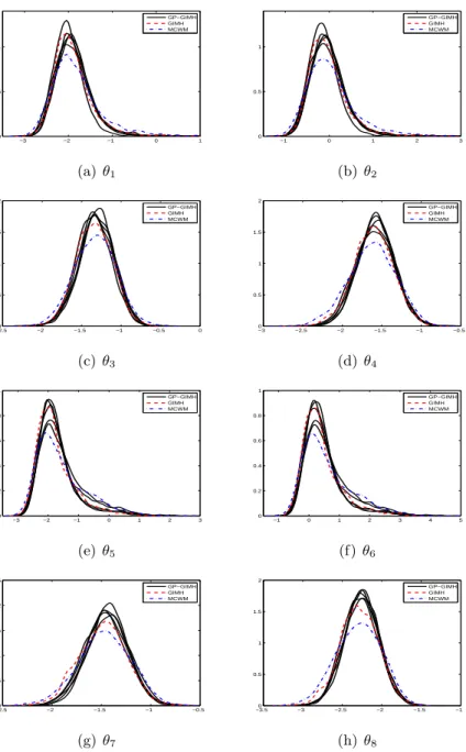
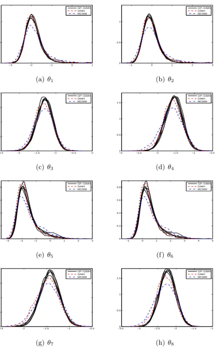
As before we find that the GP-GIMH results are generally insensitive to , though we oc-casionally observe incorrect tail behaviour when = 2; see the plots in Appendix C. The marginal posterior density estimates for the different approaches are shown in Figures 4 (with

J ≈2000 for GP-GIMH) and 5 (with J ≈4000 for GP-GIMH). Both GP-GIMH implemen-tations use a tolerance of = 1.2. It is clear that GP-GIMH provides accurate estimates of the marginal posteriors, with less between-run variability for J ≈4000. From Table 4 it is evident that GP-GIMH is capturing the true posterior correlation matrix quite accurately. In the GIMH run, there was a period where the Markov chain did not move for roughly 1700 iterations, which highlights the difficulty encountered with the GIMH approach. This likely explains the small bumps in the posteriors for θ7 and θ8 in Figures 4(g) and 4(h). With the

GP-GIMH method, as long asis set low enough, we do not observe such sticking behaviour. Table 5 shows the run times (averaged over the five independent runs) for GP-GIMH for different combinations ofJ and . Note that these times exclude the MCWM pre-computing phase and GP fitting. Again these times appear to be fairly insensitive to the tolerance level. It is interesting to note that there is only a small increase in run times for J ≈ 4000. The increase in time for GP prediction is offset by that the fact that the GP is trained at more points so that unreliable GP predictions (withs∗(θ∗)> ) occur less often. Furthermore, there is lower variability in the run times with J ≈ 4000: in the fifteen runs of GP-GIMH with

J ≈4000 (five independent runs for each of three different values) the standard deviation of the run time is 0.9 hours whereas the corresponding number forJ ≈2000 is 1.3 hours. The computational, statistical and overall efficiency of the different approaches is shown in

−3 −2 −1 0 1 0 0.5 1 GP−GIMH GIMH MCWM (a)θ1 −1 0 1 2 3 0 0.5 1 GP−GIMH GIMH MCWM (b) θ2 −2.50 −2 −1.5 −1 −0.5 0 0.5 1 1.5 2 GP−GIMH GIMH MCWM (c)θ3 −3 −2.5 −2 −1.5 −1 −0.5 0 0.5 1 1.5 2 GP−GIMH GIMH MCWM (d) θ4 −3 −2 −1 0 1 2 3 0 0.2 0.4 0.6 0.8 1 GP−GIMH GIMH MCWM (e)θ5 −1 0 1 2 3 4 5 0 0.2 0.4 0.6 0.8 1 GP−GIMH GIMH MCWM (f)θ6 −2.50 −2 −1.5 −1 −0.5 0.5 1 1.5 2 2.5 GP−GIMH GIMH MCWM (g)θ7 −3.50 −3 −2.5 −2 −1.5 −1 0.5 1 1.5 2 GP−GIMH GIMH MCWM (h) θ8

Figure 4: Estimated marginal posterior densities for the gene network example from runs of the GIMH (red dash) and MCWM (blue dash-dot) algorithms and five independent runs of the GP-GIMH (black solid) algorithm withJ ≈2000 and= 1.2.

−3 −2 −1 0 1 0 0.5 1 GP−GIMH GIMH MCWM (a)θ1 −1 0 1 2 3 0 0.5 1 GP−GIMH GIMH MCWM (b) θ2 −2.50 −2 −1.5 −1 −0.5 0 0.5 1 1.5 2 GP−GIMH GIMH MCWM (c)θ3 −3 −2.5 −2 −1.5 −1 −0.5 0 0.5 1 1.5 GP−GIMH GIMH MCWM (d) θ4 −3 −2 −1 0 1 2 3 0 0.2 0.4 0.6 0.8 GP−GIMH GIMH MCWM (e)θ5 −1 0 1 2 3 4 5 0 0.2 0.4 0.6 0.8 GP−GIMH GIMH MCWM (f)θ6 −2.50 −2 −1.5 −1 −0.5 0.5 1 1.5 2 GP−GIMH GIMH MCWM (g)θ7 −3.50 −3 −2.5 −2 −1.5 −1 0.5 1 1.5 GP−GIMH GIMH MCWM (h) θ8

Figure 5: Estimated marginal posterior densities for the gene network example from runs of the GIMH (red dash) and MCWM (blue dash-dot) algorithms and five independent runs of the GP-GIMH (black solid) algorithm withJ ≈4000 and= 1.2.

Table 6: Comparison of the computational and statistical efficiency of the GIMH, GP-GIMH and MCWM algorithms for the gene network model. For GP-GIMH the results are averaged over the five independent runs for each combination ofJ and . † 70K iterations are used for GIMH whenN = 8000.

method acc rate (%) min ESS avg ESS time (hrs) min ESS/time avg ESS/time

GIMH (N = 4000) 7 517 700 58.0 9 12 GIMH (N = 5000) 9 689 902 77.5 9 12 GIMH (N = 6000) 10 537 984 108.3 5 9 GIMH (N = 8000)† 12 684 944 122.9 6 8 MCWM 19 445 769 120.6 4 6 J ≈2000, = 1.2 13 1074 1570 5.4 205 298 J ≈2000, = 1.5 13 915 1414 5.4 174 268 J ≈2000, = 2.0 13 538 1270 5.9 99 227 J ≈4000, = 1.2 13 994 1513 6.8 157 232 J ≈4000, = 1.5 13 1026 1513 6.6 164 243 J ≈4000, = 2.0 13 670 1297 7.2 101 191

Table 6. Again it is clear that the GP-GIMH algorithm offers generally at least an order of magnitude improvement in overall efficiency, resulting from the large reduction in computing time and a slightly higher acceptance rate than GIMH. The overall efficiency for GP-GIMH depends little onJ in this example. There is perhaps a slight decrease in overall efficiency as

increases, especially for= 2.

The GP residual plots are shown in Appendix D. As with the previous example, the normality assumption of the residuals is increasingly violated with an increase in . Again there is a small amount of curvature in some of the residuals plots, however generally the GP appears to fit reasonably well.

5.2.4 Increasing Accuracy with GP-GIMH

Finally, we attempt to use the increased efficiency of the GP-GIMH approach to target a smaller value ofσ. The idea is to obtain an approximate solution to a more accurate posterior (in the sense that it is closer to the true posterior) rather than an exact solution to a less accurate posterior. Here we setσ = 0.4 and use N = 10000 for the MCWM pre-computing step. Given the challenging nature of this problem, we use the 16 cores in the MCWM pre-computing step to obtain a more accurate log-likelihood estimate at each iteration of the MCWM phase by taking the average of 16 independent likelihood estimates. Using the 16 cores, the log-likelihood estimate has a standard deviation of roughly 2.2 at the true parameter value. The MCWM pre-computing phase is run for 2000 iterations with an adaptive MCMC strategy as detailed earlier. The maximum log-posterior is roughly -638 and we discard samples with a log-posterior below -715. We use= 1.2 for the remaining GP-GIMH algorithm with a multivariate normal proposal estimated from a few pilot runs of the method. Once the proposal distribution is determined, GP-GIMH is run for 100K iterations.

likelihood estimates required when s∗(θ∗) > can only be obtained in batches of size 1, increasing the time needed to generate these additional likelihood estimates (compounded by the fact that we use the larger N = 10000 to accommodate the smaller σ). Given the complexity of this application, we examine the impact of including for the first time a burn-in phase. Here we use B= 10000.

Since the likelihood cannot be estimated accurately even with the 16 cores here, GIMH does not perform well with N = 10000 (acceptance rate of 6% over 10K iterations). Instead we trial GIMH using N = 14000 (with this choice the standard deviation of the log-likelihood estimate is roughly 1.6 at the true value).

For GP-GIMH, the MCWM phase takes 10 hours. The remaining part of the GP-GIMH algorithm takes 6.75 hours without the burn-in phase and 3.25 hours with the burn-in phase. The improvement in computing time afforded with the burn-in more than outweighs the fact that 10K less iterations can be used for inference. Appendix E shows that the posterior estimates obtained by GP-GIMH depend very little on whether a burn-in is used. The GIMH method takes roughly 80 hours to run only 20K iterations. Further, there is a dramatic reduction in acceptance rate, down from 35% for GP-GIMH to 13% for GIMH (note that this is even with smaller random walk standard deviations to improve the acceptance rate). This amounts to an efficiency improvement of roughly 90 times for GP-GIMH (with burn-in) over GIMH (and 70 times without the burn-in).

Posterior distribution estimates are shown in Figure 6 for GP-GIMH (σ = 0.4 with burn-in phase) and GIMH (for both σ = 0.6 and σ = 0.4). It is important to note that the GIMH posterior estimates withσ = 0.4 are rough as they are based on a low ESS (average ESS over parameters of about 80). There is a marked shift in the posteriors towards the true values for θ3 and θ7 when σ is reduced to 0.4, which the GP-GIMH approach is able to capture

accurately. There is a gain in precision forθ4 andθ8, which GP-GIMH is also able to capture.

The GP-GIMH approach is recovering the skewed posteriors (θ1, θ2, θ7 and θ8) with less

accuracy, with the method appearing to spend too much time in the right tails. Overall, the GP-GIMH method is performing well here given the massive improvement in efficiency. The results of GIMH suggest that the posteriors are moving away from the true parameter values for θ1 and θ2 when σ is reduced. This might be explained by the fact that only a

relatively small dataset is used here, and so the parameter values most favourable for the dataset generated may be away from the true parameter values.

6

Discussion

In this paper we have presented an approach to accelerate pseudo-marginal methods using GPs. The main idea is to use the well-mixing and conservative MCWM algorithm to train the GP, and then replace expensive likelihood approximations with cheap GP predictions in the GIMH algorithm. We find that the method is able to produce reasonable estimates of the marginal posterior distributions and the posterior correlation matrix of a stochastic volatility model and a gene network model with at least an order of magnitude improvement in computing time. For the gene network example, we demonstrate how the efficiency gains can be directed to obtain an approximation to a more accurate posterior distribution.

−3 −2 −1 0 1 0 0.5 1 1.5 GP−GIMH σ = 0.4 GIMH σ = 0.4 GIMH σ = 0.6 (a)θ1 −1 0 1 2 3 0 0.5 1 GP−GIMH σ = 0.4 GIMH σ = 0.4 GIMH σ = 0.6 (b) θ2 −2.50 −2 −1.5 −1 −0.5 0 0.5 1 1.5 2 2.5 3 3.5 GP−GIMH σ = 0.4 GIMH σ = 0.4 GIMH σ = 0.6 (c)θ3 −3 −2.5 −2 −1.5 −1 −0.5 0 0.5 1 1.5 2 2.5 GP−GIMH σ = 0.4 GIMH σ = 0.4 GIMH σ = 0.6 (d) θ4 −3 −2 −1 0 1 2 3 0 0.2 0.4 0.6 0.8 GP−GIMH σ = 0.4 GIMH σ = 0.4 GIMH σ = 0.6 (e)θ5 −1 0 1 2 3 4 5 0 0.2 0.4 0.6 0.8 1 GP−GIMH σ = 0.4 GIMH σ = 0.4 GIMH σ = 0.6 (f)θ6 −2.50 −2 −1.5 −1 −0.5 0.5 1 1.5 2 2.5 GP−GIMH σ = 0.4 GIMH σ = 0.4 GIMH σ = 0.6 (g)θ7 −3.50 −3 −2.5 −2 −1.5 −1 0.5 1 1.5 2 2.5 3 GP−GIMH σ = 0.4 GIMH σ = 0.4 GIMH σ = 0.6 (h) θ8

Figure 6: Estimated marginal posterior densities for the gene network example from GIMH with σ = 0.6 (red dash) and GP-GIMH with σ = 0.4 and a burn-in phase of B = 10000 iterations (black solid).

Below we discuss various practical considerations and some future research directions that we plan to consider.

6.1 Practical Considerations

Although we are specific about the GP choices adopted here, as we find them to be successful for the example considered in Section 5, other choices for the mean function, covariance function and observation model may be selected. Such selections are likely to be problem dependent, for example some noisy log-likelihood functions might be better modelled with an error variance that depends onθ, such as heteroscedastic GP models (Goldberg et al., 1998; Kersting et al., 2007). In practice one may use a model selection procedure (Rasmussen and Williams, 2006, chap. 5) to determine the most appropriate GP for a given training sample. However, a more sophisticated GP will result in more complex computations involving the GP. This requires further investigation.

We tried several different approaches when the GP prediction was too uncertain. At such proposed values, we considered instead estimating the likelihood precisely using a large value ofN, rather than relying on the GP to provide a prediction. The idea is that such expensive likelihood evaluations are only required comparatively less often. We found that this ap-proach was somewhat successful, but was slower in general and resulted in some unusual tail behaviour compared with the approach adopted in the paper, which involves (temporarily) adding likelihood estimations to the training sample. We also considered continually expand-ing the trainexpand-ing sample with likelihood estimations when required so that the GP can become more certain across a wider parameter space. However, adding to the training samples in this way affects the fit of the GP at values already processed in the GP-GIMH algorithm, thus the target distribution of the method is continually moving. This resulted in unusual trace plots. We found that including a burn-in phase where adaptation could take place but not thereafter was a useful compromise. Other methods that have incorporated adaptation, such as Conrad et al. (2015), have used approximations with local support so that the effect of the changes were contained. In the same spirit, re-estimating GP hyperparameters after appending additional training samples resulted in similarly strange trace plots.

In this article we have not investigated the optimal standard deviation of the log-likelihood estimator to use in the MCWM pre-computing phase. Such an investigation would require an extensive and significant simulation study. Here we found success when the standard deviation of the log-likelihood estimator is roughly 2 in the MCWM pre-computing phase. This is of interest as it is larger than that recommended for GIMH (Doucet et al., 2015), which suggests that our approach should be useful in complex scenarios.

6.2 Future Work

We used the same proposal distribution to enable comparison of statistical efficiency between the three methods. The covariance matrix for the multivariate normal random walk was determined from some pilot runs, which worked well for our application. Alternatively, the precomputed approximation to the log-likelihood could also be used to design improved pro-posals for GP-GIMH. The covariance function of the GP could be viewed as a smoothed

representation of the geometry of the parameter space. Where there is strong dependence between parameters, information such as gradient and curvature can be utilised to propose large moves with high acceptance probability. For example, Zhang et al. (2015) incorpo-rate a precomputation step in their approximate Hamiltonian Monte Carlo method (see also Rasmussen (2003)).

The ideas of this paper could be extended to construct a Bayesian optimisation algorithm (Jones et al., 1998) in order to perform approximate maximum likelihood estimation in models where only a likelihood estimator is used. Confidence intervals for parameter estimates could be approximated via the profile likelihood or with the parametric bootstrap (e.g. Efron and Tibshirani, 1986). The MCWM algorithm with a uniform prior distribution could be run to initially train the GP.

Our approach could also be used to accelerate approximate Bayesian inferences when an expensive biased likelihood estimator is used. Alquier et al. (2014) present a noisy MCMC framework that provides bounds on the error when a biased likelihood estimator is used in an MCMC method. Another example is the synthetic likelihood of Wood (2010), which assumes a multivariate normal approximation for the likelihood of a summary statistic, with a mean and covariance matrix estimated by repeated model simulation.

A GP surrogate may be incorporated into delayed-acceptance MCMC to facilitate exact Bayesian inferences in the presence of models where only an unbiased likelihood estimator is available or those with expensive likelihood functions. There is scope here to adapt the GP during the MCMC algorithm by adding training samples when necessary and/or re-estimating hyperparameters.

If exact results are necessary, the output of our GP-GIMH approach may be used to form an importance distribution for importance sampling (IS) or sequential Monte Carlo (SMC). The IS and SMC approaches have been extended to allow for unbiased likelihood estimators to be used (see Chopin et al. (2013), Tran et al. (2014), Duan and Fulop (2015) and Drovandi and McCutchan (2015)). The IS and SMC methods are of additional interest as they produce also an estimate of the evidence, which can be used for fully Bayesian model comparisons (see Drovandi and McCutchan (2015) and Carson et al. (2015) for examples).

References

Alquier, P., Friel, N., Everitt, R., and Boland, A. (2014). Noisy Monte Carlo: Convergence of Markov chains with approximate transition kernels. To appear in Statistics and Computing. Andrieu, C., Doucet, A., and Holenstein, R. (2010). Particle Markov chain Monte Carlo meth-ods. Journal of the Royal Statistical Society: Series B (Statistical Methodology), 72(3):269– 342.

Andrieu, C. and Roberts, G. O. (2009). The pseudo-marginal approach for efficient Monte Carlo computations. The Annals of Statistics, 37(2):697–725.

Beaumont, M. A. (2003). Estimation of population growth or decline in genetically monitored populations. Genetics, 164(3):1139–1160.

Carson, J., Crucifix, M., Preston, S., and Wilkinson, R. D. (2015). Bayesian model selection for the glacial-interglacial cycle. arXiv:1511.03467v1.

Chopin, N., Jacob, P. E., and Papaspiliopoulos, O. (2013). SMC2: an efficient algorithm for sequential analysis of state space models. Journal of the Royal Statistical Society: Series B (Statistical Methodology), 75(3):397–426.

Christen, J. A. and Fox, C. (2005). Markov chain Monte Carlo using an approximation.

Journal of Computational and Graphical Statistics, 14(4):795–810.

Conrad, P. R., Marzouk, Y. M., Pillai, N. S., and Smith, A. (2015). Accelerating asymp-totically exact MCMC for computationally intensive models via local approximations.

arXiv:1402.1694v4.

Doucet, A., Pitt, M., and Kohn, R. (2015). Efficient implementation of Markov chain Monte Carlo when using an unbiased likelihood estimator. To appear in Biometrika.

Drovandi, C. C. (2014). Pseudo-marginal algorithms with multiple CPUs.

http://eprints.qut.edu.au/61505/.

Drovandi, C. C. and McCutchan, R. A. (2015). Alive SMC2: Bayesian model selection for low-count time series models with intractable likelihoods. To appear in Biometrics. Duan, J.-C. and Fulop, A. (2015). Density-tempered marginalized sequential Monte Carlo

samplers. Journal of Business & Economic Statistics, 33(2):192–202.

Efron, B. and Tibshirani, R. (1986). Bootstrap methods for standard errors, confidence intervals, and other measures of statistical accuracy. Statistical Science, 1(1):54–75. Fearnhead, P., Giagos, V., and Sherlock, C. (2014). Inference for reaction networks using the

linear noise approximation. Biometrics, 70(2):457–466.

Goldberg, P. W., Williams, C. K. I., and Bishop, C. M. (1998). Regression with input-dependent noise: a Gaussian process treatment. InAdv. Neural Inf. Process. Syst. (NIPS), volume 10, pages 493–499. The MIT Press.

Golightly, A., Henderson, D. A., and Sherlock, C. (2015). Delayed acceptance particle MCMC for exact inference in stochastic kinetic models. Statistics and Computing, 25(5):1039–1055. Golightly, A. and Wilkinson, D. J. (2005). Bayesian inference for stochastic kinetic models

using a diffusion approximation. Biometrics, 61(3):781–788.

Gordon, N. J., Salmond, D. J., and Smith, A. F. M. (1993). Novel approach to nonlinear/non-Gaussian Bayesian state estimation. In Radar and Signal Processing, IEE Proceedings F, volume 140, pages 107–113.

Holenstein, R. (2009). Particle Markov Chain Monte Carlo. PhD thesis, The University Of British Columbia.

Jones, D. R., Schonlau, M., and Welch, W. J. (1998). Efficient global optimization of expensive black-box functions. Journal of Global Optimization, 13(4):455–492.

Kennedy, M. C. and O’Hagan, A. (2000). Predicting the output from a complex computer code when fast approximations are available. Biometrika, 87(1):1–13.

Kennedy, M. C. and O’Hagan, A. (2001). Bayesian calibration of computer models. Journal of the Royal Statistical Society: Series B (Statistical Methodology), 63(3):425–464.

Kersting, K., Plagemann, C., Pfaff, P., and Burgard, W. (2007). Most likely heteroscedastic Gaussian process regression. InProc. 24th Int. Conf. Mach. Learn. (ICML), volume 227 of

ACM International Conference Proceeding Series, pages 393–400.

Plummer, M., Best, N., Cowles, K., and Vines, K. (2006). CODA: Convergence diagnosis and output analysis for MCMC. R News, 6(1):7–11.

Rasmussen, C. E. (2003). Gaussian processes to speed up hybrid Monte Carlo for expensive Bayesian integrals. In Bernardo, J., Bayarri, M., Berger, J., Dawid, A., Heckerman, D., Smith, A., and West, M., editors, Bayesian Statistics, volume 7, pages 651–659.

Rasmussen, C. E. and Williams, C. K. I. (2006). Gaussian processes for machine learning. The MIT Press, Cambridge, Massachusetts.

Sherlock, C., Golightly, A., and Henderson, D. A. (2015). Adaptive, delayed-acceptance MCMC for targets with expensive likelihoods. arXiv:1509.00172v1.

Tran, M.-N., Nott, D. J., and Kohn, R. (2015). Variational Bayes with intractable likelihood.

arXiv:1503.08621v1.

Tran, M.-N., Scharth, M., Pitt, M. K., and Kohn, R. (2014). Importance sampling squared for Bayesian inference in latent variable models. Available at SSRN 2386371.

Wilkinson, R. (2014). Accelerating ABC methods using Gaussian processes. Journal of Machine Learning Research, 33:1015–1023.

Wood, S. N. (2010). Statistical inference for noisy nonlinear ecological dynamic systems.

Nature, 466:1102–1107.

Zhang, C., Shahbaba, B., and Zhao, H. (2015). Precomputing strategy for Hamiltonian Monte Carlo method based on regularity in parameter space. arXiv:1504.01418v1.

Appendices for Accelerating Pseudo-Marginal MCMC using

Gaussian Processes

C. C. Drovandi*, M. T. Moores and R. J. Boys

*Queensland University of Technology, Brisbane, Australia 4001 email: [email protected]

Appendix A

−0.10 −0.05 0 0.05 0.1 5 10 15 20 25 −0.40 −0.2 0 0.2 2 4 6 8 0.2 0.3 0.4 0.5 0.6 0 2 4 6 8 10 12 0 0.05 0.1 0.15 0 10 20 30 40 50 0 0.01 0.02 0.03 0 50 100 150

Figure 1: Sensitivity to for the stochastic volatility example for the first independent run whenJ ≈1500. Posterior estimates are shown for= 1.0 (black),= 1.5 (blue) and = 2.0 (red).

−0.10 −0.05 0 0.05 0.1 5 10 15 20 25 −0.40 −0.2 0 0.2 2 4 6 8 0.2 0.3 0.4 0.5 0.6 0 2 4 6 8 10 12 0 0.05 0.1 0.15 0 10 20 30 40 0 0.01 0.02 0.03 0 50 100 150

Figure 2: Sensitivity tofor the stochastic volatility example for the second independent run whenJ ≈1500. Posterior estimates are shown for= 1.0 (black),= 1.5 (blue) and = 2.0 (red).

−0.10 −0.05 0 0.05 0.1 5 10 15 20 25 −0.40 −0.2 0 0.2 2 4 6 8 0.2 0.3 0.4 0.5 0.6 0 5 10 15 0 0.05 0.1 0.15 0 10 20 30 40 50 0 0.01 0.02 0.03 0 50 100 150

Figure 3: Sensitivity to for the stochastic volatility example for the third independent run whenJ ≈1500. Posterior estimates are shown for= 1.0 (black),= 1.5 (blue) and = 2.0 (red).

−0.10 −0.05 0 0.05 0.1 5 10 15 20 25 −0.40 −0.2 0 0.2 2 4 6 8 0.2 0.3 0.4 0.5 0.6 0 2 4 6 8 10 12 0 0.05 0.1 0.15 0 10 20 30 40 50 0 0.01 0.02 0.03 0 50 100 150

Figure 4: Sensitivity tofor the stochastic volatility example for the fourth independent run whenJ ≈1500. Posterior estimates are shown for= 1.0 (black),= 1.5 (blue) and = 2.0 (red).

−0.10 −0.05 0 0.05 0.1 5 10 15 20 25 −0.40 −0.2 0 0.2 2 4 6 8 0.2 0.3 0.4 0.5 0.6 0 2 4 6 8 10 12 0 0.05 0.1 0.15 0 10 20 30 40 0 0.01 0.02 0.03 0 50 100 150

Figure 5: Sensitivity to for the stochastic volatility example for the fifth independent run whenJ ≈1500. Posterior estimates are shown for= 1.0 (black),= 1.5 (blue) and = 2.0 (red).

−0.10 −0.05 0 0.05 0.1 5 10 15 20 25 −0.40 −0.2 0 0.2 2 4 6 8 0.2 0.3 0.4 0.5 0.6 0 2 4 6 8 10 12 0 0.05 0.1 0.15 0 10 20 30 40 50 0 0.01 0.02 0.03 0 50 100 150

Figure 6: Sensitivity to for the stochastic volatility example for the first independent run whenJ ≈3000. Posterior estimates are shown for= 1.0 (black),= 1.5 (blue) and = 2.0 (red).

−0.10 −0.05 0 0.05 0.1 5 10 15 20 25 −0.40 −0.2 0 0.2 2 4 6 8 0.2 0.3 0.4 0.5 0.6 0 2 4 6 8 10 12 0 0.05 0.1 0.15 0 10 20 30 40 0 0.01 0.02 0.03 0 50 100 150

Figure 7: Sensitivity tofor the stochastic volatility example for the second independent run whenJ ≈3000. Posterior estimates are shown for= 1.0 (black),= 1.5 (blue) and = 2.0 (red).