Compact, diverse and efficient: globular cluster binaries and gravitational wave parameter estimation challenges

COMPACT, DIVERSE

AND EFFICIENT:

GLOBULAR CLUSTER BINARIES

AND GRAVITATIONAL WAVE

PARAMETER ESTIMATION

CHALLENGES

CARL-JOHAN OLOF HASTER

A thesis submitted to the

University of Birmingham

for the degree of

DOCTOR OF PHILOSOPHY

Astrophysics and Space Research

School of Physics and Astronomy

College of Engineering and Physical Sciences

University of Birmingham

April 2016

University of Birmingham Research Archive

e-theses repository

This unpublished thesis/dissertation is copyright of the author and/or third parties. The intellectual property rights of the author or third parties in respect of this work are as defined by The Copyright Designs and Patents Act 1988 or as modified by any successor legislation.

Any use made of information contained in this thesis/dissertation must be in accordance with that legislation and must be properly acknowledged. Further distribution or reproduction in any format is prohibited without the permission of the copyright holder.

Acknowledgements

It is my sincere pleasure to thank the following people: Min bror Erik, mamma Kerstin och pappa Lars-Olof, utan ert stöd och hjälp hade jag aldrig v ˙agat tro att detta hade varit möjligt. My supervisors Ilya Mandel and Alberto Vecchio for their mentorship, support and endless patience; Christopher Berry, Walter Del Pozzo, Will Farr, John Veitch, Alberto Sesana and David Stops for providing both interesting discussions and answers to my many questions. Fabio Antonini, Katie Breivik , Sourav Chatterjee, Ben Farr, Vicky Kalogera, Tyson Littenberg, Fred Rasio and Carl Rodriguez for making my months in Chicago both fun, interesting and memorable. All my friends in the ASR group at Birmingham, especially Jim Barrett, Charlotte Bond, Daniel Brown, Mark Burke, Chris Collins, Sam Cooper, Sebastian Gaebel, Anna Green, Kat Grover, Maggie Lieu, Hannah Middleton, Chiara Mingarelli, Sarah Mulroy, Trevor Sidery, Rory Smith, Simon Stevenson, Daniel Töyrä, Alejandro Vigna-Gómez and Serena Vinciguerra for years of fun and adventures; The members of the CBC group, and specifically the Parameter Estimation subgroup, for all their help. I would also like to thank Alberto Sesana and Jonathan Gair for their great skill and patience as the examiners for my PhD viva.

Several of the chapters in this thesis were the result of collaborations and benefited from discussions with several people. Chapter 2 was based on work done in collaboration with Fabio Antonini, Ilya Mandel and Vicky Kalogera [108], and benefited from discussions with Sourav Chatterjee, Jonathan Gair, James Guillochon, Fred Rasio and Alberto Sesana. Chapter 3 was based on work done in collaboration with Zhilu Wang, Christopher Berry, Simon Stevenson, John Veitch and Ilya Mandel [110] and benefited from discussions with Michael Pürrer, Tom Callister and Tom Dent. Chapter 4 was based on work done in collaboration

with Ilya Mandel and Will M. Farr [109], and benefited from discussions with Christopher Berry, Walter Del Pozzo, Alberto Vecchio, John Veitch, Richard O’Shaughnessy and Chris Pankow.

My work has been supported by a studentship from the University of Birming-ham and the Center for Interdisciplinary Exploration in Astrophysics at North-western University.

Abstract

Following the first detection of gravitational waves from a binary coa-lescence the study of the formation and evolution of these gravitational-wave sources and the recovery and analysis of any detected event will be crucial for the newly realised field of observational gravitational wave astrophysics.

This thesis covers a wide range of these topics including simulating the dense environments where compact binaries are likely to form, focus-ing on binaries containfocus-ing an intermediate mass black hole (IMBH). It is shown that such binaries do form, are able to merge within a

∼ 100 Myr simulation, and that the careful treatment of the orbital evolution (including post-Newtonian effects) implemented here was crucial for correctly describing the binary evolution. The later part of the thesis covers the analysis of the gravitational waves emitted by such a binary, and shows it is possible to identify the IMBH with high confidence, together with most other parameters of the binary, despite the short-duration signals and assumed uncertainties in the available waveform models. Finally a method for rapid parameter es-timation of gravitational wave sources is presented and shown to re-cover source parameters with comparable accuracy using only a small fraction ∼ 0.1% of the computational resources required by conven-tional methods.

Contents

Acknowledgements i

Contents iv

List of Figures vii

1 Introduction 1

1.1 Compact binary formation . . . 2

1.1.1 Binary stellar evolution . . . 2

1.1.2 Dynamical formation . . . 4 1.2 Gravitational waves . . . 4 1.2.1 General relativity . . . 4 1.2.2 Modelling CBCs . . . 8 1.2.2.1 Inspiral . . . 8 1.2.2.2 Merger . . . 13 1.2.2.3 Ringdown . . . 13 1.2.2.4 Complete CBC waveform . . . 13 1.3 Data analysis . . . 14 1.3.1 searches . . . 14 1.3.2 PE . . . 21 1.3.2.1 MCMC . . . 23 1.3.2.2 Nested Sampling . . . 25 1.4 Structure of thesis . . . 29 1.4.1 Chapter 2 . . . 29 1.4.2 Chapter 3 . . . 30

CONTENTS

1.4.3 Chapter 4 . . . 31

2 N−body dynamics of Intermediate mass ratio inspirals 32 2.1 Introduction . . . 32

2.2 Simulations . . . 34

2.3 Results . . . 35

2.4 Discussion . . . 45

2.5 Conclusion . . . 49

3 Inference on gravitational waves from coalescences of stellar-mass compact objects and intermediate-stellar-mass black holes 55 3.1 Introduction . . . 55

3.2 Study design . . . 57

3.2.1 Sources and sensitivity . . . 58

3.2.2 Parameter estimation . . . 59

3.3 Key results . . . 60

3.3.1 Effects of cosmology on inferring the presence of an IMBH 68 3.4 Discussion . . . 69

3.4.1 Impact of low-frequency sensitivity . . . 70

3.4.2 Uncertainty versus signal-to-noise ratio . . . 70

3.4.3 Systematics . . . 74

3.5 Summary . . . 78

4 Efficient method for measuring the parameters encoded in a gravitational-wave signal 80 4.1 Introduction . . . 80

4.1.1 Binary coalescence model . . . 81

4.1.2 Bayesian inference . . . 82

4.1.3 Stochastic sampling . . . 83

4.1.4 Chapter organisation . . . 84

4.2 Discretizing the credible regions . . . 84

4.2.1 Cumulative posterior on a grid . . . 85

4.2.2 Grid placement . . . 85

CONTENTS

4.3 Comparison with alternative methods: which approximations are warranted? . . . 90

4.3.1 Cumulative likelihood . . . 90

4.3.2 Iso-Match contours and the Linear Signal Approximation . 92

4.3.3 Comparasion . . . 95

4.4 Conclusions and future directions . . . 95

5 Conclusion 101

List of Figures

1.1 Formation of a binary black hole in the galactic field . . . 3

1.2 Formation of a binary black hole under chemically homogeneous evolution . . . 5

1.3 Dynamical formation of a binary black hole . . . 6

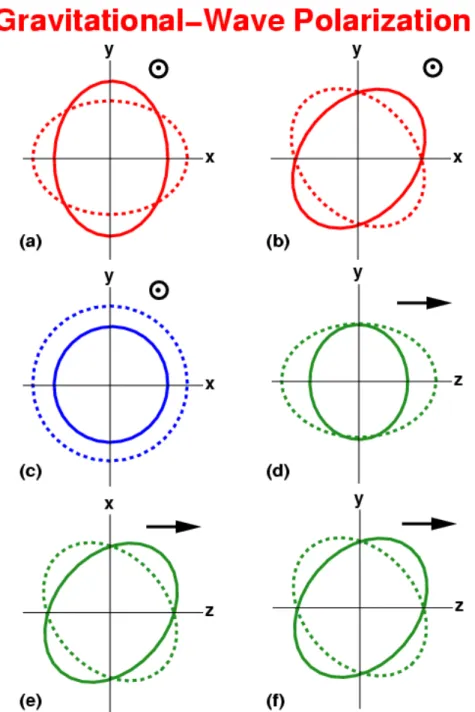
1.4 Gravitational wave polarisations . . . 9

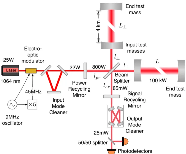
1.5 Layout of an aLIGO interferometer . . . 10

1.6 An example CBC waveform in the time domain . . . 14

1.7 aLIGO noise budget . . . 15

1.8 Amplitude spectral densities for LIGO . . . 16

1.9 Relative orientation of an interferometer and a gravitational wave source . . . 19

1.10 Example CBC waveforms in the frequency domain . . . 20

1.11 Likelihood contours in nested sampling . . . 26

1.12 Nested sampling live points . . . 28

2.1 Black hole distance to cluster center of mass . . . 36

2.2 Black hole distance to the IMBH . . . 37

2.3 IMBH–BH binary semi-major axis . . . 39

2.4 IMBH–BH binary eccentricity . . . 51

2.5 IMBH–BH–BH triple inclination . . . 52

2.6 The merger trajectory for the IMBH–BH binary . . . 53

2.7 Detection horizon distance and comoving volume . . . 54

3.1 90% credible intervals for chirp mass . . . 61

LIST OF FIGURES

3.3 Ratio of 90% credible intervals for chirp mass and total mass . . . 63

3.4 90% credible intervals for binary component masses . . . 65

3.5 90% credible intervals for the dominant ringdown frequency . . . 66

3.6 90% credible intervals for the effective spin . . . 67

3.7 Fraction of msource 1 posterior above MIMBH . . . 69

3.8 Characteristic strain and noise amplitudes . . . 71

3.9 Accumulated SNR below the frequency fcut. . . 72

3.10 90% credible intervals for the mass ratio varying the low-frequency bound . . . 73

3.11 Example posterior probability density functions . . . 75

3.12 Credible interval scaling with SNR . . . 76

3.13 Comparison of systematic effects caused by waveform uncertainty 77 4.1 Credible regions for a cumulative marginalized posterior . . . 89

4.2 Credible regions for a cumulative maximized likelihood . . . 91

4.3 Credible regions according to iso-match contours . . . 94

4.4 Comparison of credible region estimate methods . . . 96

4.5 Credible regions for a cumulative marginalized posteirior, free ex-trinsic parameters . . . 98

Chapter 1

Introduction

The scientific field of observational gravitational wave astrophysics was, a century after the initial theoretical predictions [82,83], initiated by the observation of the coalescence of a system of binary black holes named GW150914 [22]. Although there were indirect observational evidence of emission of gravitational waves from the orbital evolution of binary pulsar systems [119, 251, 130], GW150914 was the first direct probe into the dark realm of strong-field gravitational physics. This observation had not been possible without the design, construction and commissioning of the laser interferometer detectors of Advanced LIGO [aLIGO;

13] which performed their first observational run, O1, between September 12, 2015 and January 19, 2016. Together with the future detectors of Advanced Virgo [AdV; 27], KAGRA [221] and LIGO India [122], aLIGO will form a global network of gravitational wave observatories operating in the Hz to kHz frequency range, sensitive to some of the most energetic events in the universe. One of the primary sources for gravitational waves detectable by such a network are the coalescences of compact objects in binary systems (CBCs). This includes binaries containing either only neutron stars (BNS), black holes (BBH) or a combination (NSBH).

1.1

Formation and evolution of compact

binaries

Previous observations of compact objects have been done in the electromagnetic spectrum, e.g. both black holes and neutron stars as members of x-ray binaries [141] and neutron stars also as radio pulsars [143]. These observations have been used to inform models for estimated coalescence rates, which can then be converted into predictions of rates of detected events in aLIGO. Even after the observation of GW150914 the estimated rates of BBH coalescences is uncertain [2−400Gpc−3yr−1from23], and the non-detection of NSBH or BNS systemsso far

in aLIGO leaves the estimated rates at their pre-O1 state [0.6−1000 Gpc−3yr−1 and 10 −104 _Gpc−3_yr−1 _{respectively, from 17], these estimations are however}

expected to change after the final search results from O1 have been published. An interesting feature among the observed compact objects are that there appears to be a “mass gap” between the heaviest observed neutron star [at just above 2M, see 133] and the lightest black hole [at ∼ 4 −5.5M, 179, 85, depending on the assumed mass distibution]. There are however arguments for whether the gap is physical [48, and indicative of specifics within supernova en-gines] or caused by observational selection effects [131]. While future observations of gravitational waves from CBCs with components near or inside the mass gap will give the final verdict on its existence, they will also provide information about the underlying formation and evolution of compact objects [154,140].

1.1.1

Binary formation from stellar evolution in the

galactic field

It has been observed that a majority of stars massive enough to form compact ob-jects are found in binary systems [205, 127]. These observations, combined with models for stellar evolution (both of the individual stars and their binary inter-actions [124,244,191, and seeFigure 1.1]), can then be used for large scale simu-lations of realistic popusimu-lations of compact binary systems [46,44,76–78,222,47] [and see45, for the implications specific to the formation of GW150914]. In addi-tion to the “convenaddi-tional” BBH formaaddi-tion paths for stellar binaries in a galactic

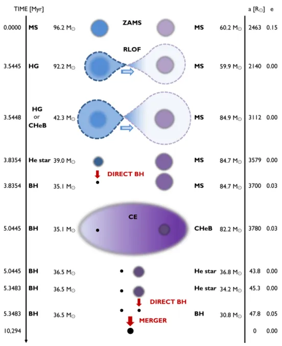
Figure 1.1 After the formation of a binary containing two massive stars, the pair experiences stable mass transfer through the overflow of the Roche lobe for the system. The initially most massive star undergoes core-collapse into a black hole after which an additional mass transfer phase forms a common envelope that, through dynamical friction, hardens the binary further. After the second star forms a black hole, through another core-collapse, the orbital evolution of the binary becomes dominated by emission of gravitational waves which leads to an inspiral and a subsequent merger. Figure reproduced from [45]

field population described in Figure 1.1 recent studies have suggested another formation method. There the helium formed in the stellar core is homogeneously mixed throughout the star, through its rapid rotation, keeping the star compact throughout its lifetime. This formation channel could therefore more easily give rise to more massive black holes than the “normal evolution” path [152,75, 157, and see Figure 1.2].

1.1.2

Dynamical binary formation in dense stellar

envi-ronments

Where the formation of binary compact objects through stellar evolution in the galactic field is found to be highly dependant on the specific modelling of the binary interactions of the evolving stars, it is also possible to produce CBCs in dense stellar environments, such as globular clusters, where the formation is dominated by the much more clearly understood gravitational dynamics, an example is shown in Figure 1.3. Simulations which include both a treatment of stellar evolution and a realistic description (size, mass and number of particles) of globular clusters have primarily been performed using Monte Carlo methods [79, 80, 171, 170, 202, 198, 67] but comparisons against more computationally intensive direct N-body simulations have shown excellent agreement [203] [and see 200, for the implications specific to the formation of GW150914].

1.2

Gravitational wave sources

1.2.1

General relativity

Gravitational waves, labelled here as h, can be regarded as a small time-varying perturbation on the flat Minkowskian metric, η, to give a total metric g with components, for spacetime coordinates µ, ν, given as

gµ,ν =hµ,ν +ηµ,ν (1.1)

which is observed as a dimensionless transverse strain in the local spacetime. This strain h is to leading order determined by the second time derivative of the

H rich H rich He rich H rich He Roche lobe overflow 2-b 3-b 3-a chemically homogeneous evolution normal evolution He rich He 4-a BH 1 2-a Merger or severe mass loss by Roche-lobe overflow

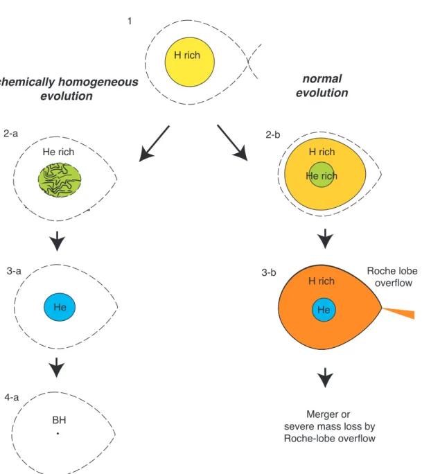
Figure 1.2 Comparing the “normal evolution” for a massive star (as also shown in

Figure 1.1) against chemically homogeneous evolution where rapid stellar rotation and tidal effects induces mixing of the helium in the core into the entire star. This suppresses stellar expansion, and thus Roche overflow and mass transfer, leading to the possible formation of more massive black holes compared to in “normal evolution”. Figure reproduced from [152]

mass quadrupole moment Qof a gravitational wave source (monopole and dipole radiation are, in general relativity, forbidden by conservation of energy and linear momentum respectively) as given by [210]

h' − G 2c4 ¨ Qij − 1 3δijQ¨kk _n inj r (1.2)

where i, j, k are the three spatial coordinates, ~n a unit vector pointing along the line of sight, r is the distance to the source and dots represent derivatives with respect to time. At leading order, the luminosity from a source emitting gravitational waves, defined as an accelerated asymmetric mass distribution, is

L= 1 5

D...

Q_jk...Q_jkE , (1.3)

where the angle brackets denote a time average over several wavelengths. For a source with characteristic mass, size, timescale and velocity M, R, T and v

respectively Equation 1.3 can be simplified to

L∼ 1 5 ... Q2 ∼ 1 5 M R2 T3 !2 ∼ 1 5 M v3 R !2 . (1.4)

or in terms of its Schwartzchild radius Rs = 2GM/c2,

L∼ LP 20 _R s R 2_v c 6 , (1.5)

which further shows that gravitational waves will be most efficient for compact (R ∼ Rs) and relativistic (v ∼ c) objects. The constant LP in Equation 1.5 is

the Planck luminosity

LP =

c5

G = 3.6×10

52_{W , (1.6)}

which is the maximum luminosity possible under general relativity, corresponding to all mass-energy in an object, M c2_{, being released in an instant and leaving}

in a light-travel time R/c. As an example, GW150914 had a peak luminosity of

∼10−3×LP which is brighter then the combined luminosity in the visible band

from all electromagnetic sources in the Universe [22].

trace-free ¨Q resulting in gravitational waves, as given by general relativity, only consisting of the transverse polarisations (a) and (b) fromFigure 1.4. One of the other distinctions between observations of gravitational waves and other forms of astronomy is that gravitational waves are observed as amplitude variations, as opposed to power fluctuations. These amplitudes, as indicated in Figure 1.4, will induce periodic variations in the distance between objects where the maxi-mum difference occurs for mutually perpendicular directions. In order to most effectively measure this differential length most modern gravitational wave detec-tors have implemented a laser Michelson interferometer, an example of which is shown in Figure 1.5. The dominating scale for a source which emits gravitational waves is set by the dimensionless orbital velocity ν ≡ vorb/c = GMtotfgw/c3.

This leads to a fundamental degeneracy between total massMtot and fgw making

shifts in mass indistinguishable from redshifts of the fgw (e.g. from cosmology) [117], this is discussed further in subsection 3.3.1. As the amplitude of h has a 1/r scaling (from Equation 1.2), this means that a gravitational wave inherently contains distance information but leaving the redshift as a model dependent free parameter.

1.2.2

Modelling compact binary coalescenses

The coalescence of a compact binary is a unique probe into strong field gravitation allowing unprecedented tests of general relativity [233]. The stringent framework provided by general relativity allows for the construction of accurate and verifiable models for the emitted gravitational waves from a compact binary coalescence.

1.2.2.1 Inspiral

During the initial phase of the coalescence the binary components are inspiraling in an orbit around their common center of mass. In this phase it is possible to represent the emitted gravitational wave amplitude to leading order as

hinspiral₀ =4ηMtotG rc2 ν 2 ≈10−231Mpc r Mc M !5/3 ω2/3 (1.7)

Figure 1.4 The six polarisation modes allowed in any metric theory of gravity for waves travelling in the +z direction. The ellipses shown represent the dis-placement of each mode on a ring of test particles. In general relativity only the transverse (a) and (b), plus and cross respectively, are allowed. For mass-less scalar–tensor theories of gravity (c), the transverse breathing mode, can be present and for massive scalar–tensor theories the longitudinal mode (d) can also be included (but suppressed relative to (c) by a factor (λ/λC) where λ is the

Photodetectors 4 km 100 kW End test mass Signal Recycling Mirror Output Mode Cleaner Beam Splitter Power Recycling Mirror 1064 nm Input Mode Cleaner Laser 25W 22W 800W 85mW Input test masses End test mass 25mW 50/50 splitter Electro-optic modulator 9MHz oscillator 5 45MHz

L

L

l

l

l

l

Figure 1.5 The layout of an aLIGO Michelson interferometer showing all optical cavities included in the design, and the associated circulating optical power in each cavity. A passing gravitational wave will introduce a difference between the two arm cavities of orderδl=Lk−L⊥. The inclusion of the arm cavities enhances the optical power in the arms by a factor Garm ' 270. Figure reproduced from

where η= (m1m2)/Mtot2 is the symmetric mass ratio, Mc = (m1m2)3/5(Mtot)−1/5

is the chirp mass (for a binary with component masses m1 and m2) and ω is the

angular frequency [147, 70]. Due to the spatial symmetry of a CBC, the emitted gravitational wave frequency fgw is twice the orbital frequency, i.e. ω = πfgw.

Equation 1.7can further be decomposed intoh+_{(t) andh}×_{(t), the two polarisation}

states allowed by general relativity (cf. Figure 1.4), as

h+(t) = 1 2h

inspiral

0 (1 + cos2ι) cos[2ϕ(t)] h×(t) =hinspiral₀ cosιsin[2ϕ(t)]

(1.8)

where ι is the inclination between the line of sight and a direction characteristic to the source (often the orbital angular momentum) and ϕ(t) corresponds to the time-dependent phase evolution of the gravitational wave source [207]. As the system is losing energy into emitted gravitational waves the orbit is shrinking, and thus the emitted frequency increases monotonically as

˙ fgw= Mc G c3 5/396 5 π 8/3 f_gw11/3 (1.9)

to leading order (this is usually called a chirp) [56]. Note, therefore, thath0 must

be a function of time as well since ν increases as the binary loses energy when its orbit shrinks. To include higher order terms the right hand side of Equa-tion 1.2 can be expanded as a Taylor series in the dimensionless orbital velocity

ν for both the amplitude and the phase of the emitted wave [55]. These post-Newtonian (pN) terms start to include (at increasingly higher order) the mass ratioq ≡m2/m1 ≤1, the components of the compact objects’ spin vectors

paral-lel to the orbital angular momentum and later the perpendicular spin components and cross correlations between these physical properties. For systems containing neutron stars, tidal effects caused by the presence of matter will also affect the orbital evolution, most prominently at the end of the inspiral phase [197]. As fgw

increases, so does ν and eventually the binary will reach a limit (ν ∼ 1) where the pN expansion no longer is valid. To ensure the accuracy of the waveforms, the inspiral phase is commonly terminated at the innermost stable circular orbit (ISCO) after which the two objects initiate the plunge towards the final merger.

The ISCO occurs, to leading order, at a fgw of fISCO = 4.4kHz _M Mtot . (1.10)

The length of a chirp is to leading order

τ '159 s _1.22M Mc 5/3 _20Hz fref !8/3 , (1.11)

wherefref is a reference frequency, usually taken as the lower bound of the detector sensitivity.

For analysis purposes, as will be further discussed in section 1.3, it is often useful to represent an inspiral waveform as its Fourier transform in the frequency domain. One commonly used representation is TaylorF2 [63] which for a face-on binary (ι = 0), with its physical parameters described by~θ, directly overhead a de-tector describes the waveform through a Taylor expansion in the post-Newtonian parameter ν as ˜ h(f, ~θ) = 1 r s 5 24π −2/3_M5/6 c f −7/6_eiΨ(f,~θ)_{, (1.12)}

assuming no higher-order corrections to the waveform amplitude. Here the phase Ψ(f, ~θ) is given as Ψ(f, ~θ) = 2πf tc−φc− π 4 + 3 128ην5 7 X k=0 (αk+βklog(ν))νk (1.13)

where tc and φc are the time and phase of the waveform at coalescence and the

coefficients αk, βk are functions of ~θ for each post-Newtonian order k/2.

An alternative expansion of Equation 1.2 comes from the effective-one-body (EOB) formalism where results from the pN approximation are supplemented by strong-field effects from the limit of a test particle inspiraling into a compact object [61, 62,72,73, 42, 225, 173]. These results are resummed into a Hamilto-nian and then improved by the inclusion of unknown higher order pN terms from numerical relativity. The current EOB waveform models can be constructed to include both generic, precessing, spin effects [180] and also tidal effects [114].

1.2.2.2 Merger

After the ISCO the analytical expressions of the inspiral are in general no longer valid. In the last decade significant breakthroughs in numerical relativity (NR) have presented solutions in general relativity which cover the merger of two (pre-viously) orbiting compact objects [192, 64, 41]. NR waveforms can now be con-structed for a variety of binary configurations (as solutions in general relativity are scale free for ∼ M f the free parameters for NR waveforms are the mass ra-tio and the spins of the two compact objects1), and are commonly collected in catalogues and used for both calibration of general waveform models as well as detailed studies of strong-field gravitation [172, 195, 112, 120, 235].

1.2.2.3 Ringdown

The merger phase of a coalescence can be taken to end the peak of the waveform, which for a BBH corresponds to when a common horizon has been formed, the resulting compact object exists in an excited spatial state. As it settles down into a stable final state the compact object radiates the excess potential energy as gravitational waves in form of a superposition of quasi-normal modes (QNMs) [81,52, 120]. To leading order, the dominant QNM emits a strain

hringdown(t)≈10−201 Mpc r M M e −t/T cos(2πf0t). (1.14) whereT = 2_{π f}1 0 andf0 '10 kHz M

M (see also the discussion around Equation 3.1

and Figure 3.5).

1.2.2.4 Complete CBC waveform

In order to fully characterise the entire coalescence of two compact objects the individual components of the inspiral–merger–ringdown are combined into a hy-bridised waveform as inFigure 1.6[176]. This is done by matching the phase and amplitude across the regions overlapping the individual waveform components, 1_{NR waveforms can also include matter effects, for example describing the tidal}

deforma-tion of neutron stars. These effects would however break the scale freedom and introduce an additional mass parameter [197].

Inspiral Merger Ringdown

post-Newtonian (PN) theory no analyt. model perturbation theory

Effective-one-body (EOB)

Numerical Relativity (NR)

Figure 1.6 Showing an example waveform in the time domain for a BBH system with non-spinnning components. As the analytically described inspiral phase breaks down the waveform is required to be hybridised against a NR solution. After this merger phase, indicated by the wavy line, the emitted waveform can again be explained analytically through a superposition of QNMs. Figure repro-duced from [176].

either using a phenomenological model [208, 104, 209, 120, 126] or more directly within the EOB framework [225,180,114].

1.3

Gravitational wave data analysis

Although ground-based gravitational wave detectors are sensitive to a wide vari-ety of sources (e.g. unmodelled bursts [14, 4, 15, 10, 18, 231], continuous waves [5, 2, 7, 3, 8] and stochastic signals [24, 16, 9, 6, 20]) this thesis will focus only on the data analysis in use for compact binary coalescence signals.

1.3.1

Searches for CBC

A typical CBC signal detectable in aLIGO can be expected to induce strains of order h∼10−23∼δl/l, which for the arm lengths ofl ∼few km for aLIGO/AdV requires a differential arm length ofδl∼10−20_{m to be reliably measurable. This}

can be translated directly into requirements on the stability and sensitivity of the detectors [106]. As it has been demonstrated during the fall of 2015, the aLIGO detectors have achieved a level of sensitivity enough to claim a detection of at least one CBC event [22, 21, 229]. The detector sensitivity is limited in different frequency bands by different noise sources, as shown inFigure 1.7. At low

Measured Quantum Thermal Seismic Newtonian Other DOF 10 100 1000 10-20 10-19 10-18 10-17 10-16 Frequency(Hz) Displacement ( m / Hz )

Figure 1.7 Showing in red the measured sensitivity to displacements δl in the Hanford detector during the first observational run of aLIGO. This measured sensitivity is accounted for, as a sum of the individual noise components, for the majority of the sensitive frequency band, apart from between 20 _. f _.100 Hz. Figure reproduced from [21].

10

2

₁₀

3

Frequency, Hz

10

-24

10

-23

10

-22

10

-21

St

ra

in

n

oi

se

, 1

/H

z

1

/

2

Advanced LIGO, L1 (2015)

Advanced LIGO, H1 (2015)

Enhanced LIGO (2010)

Advanced LIGO design

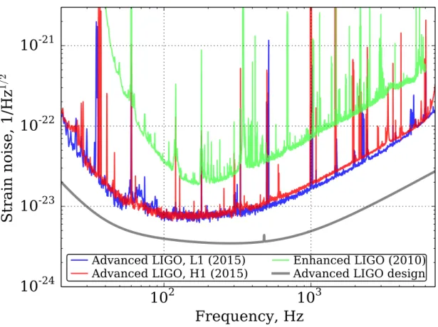
Figure 1.8 The measured noise amplitude spectral density represented as a strain sensitivity for the two aLIGO detectors, H1 and L1, during the first observational run in 2015. Also shown are the final sensitivity of the initial LIGO detectors as well as the predicted design sensitivity for aLIGO. Figure reproduced from [229].

frequencies the noise is dominated by seismic ground motion, thermal (Brownian) noise in the mirror, coatings and suspensions and cross coupled noises originating in the interferometer control system (labeled “other DOF” in Figure 1.7). At higher frequencies the noise budget is instead completely dominated by quantum effects such as shot noise and radiation pressure caused by uncertainties in the photon count inside the interferometer and the photon arrival time at the readout. By dividing the displacement sensitivity by the arm length (l = 4 km for aLIGO) a noise amplitude spectral density (ASD) is produced, examples of which is shown in Figure 1.8. This can more easily be compared directly to a CBC strain signal as shown in Figure 1.10[see 168, for a comprehensive comparison].

pipelines it is considered to be Gaussian and stationary over a timescale of any given CBC signal (∼seconds to minutes). In practice this is not the case, see for example section III.D in [11] and section III.K in [229] for further discussion, and a large effort is put towards towards characterising and mitigating these effects in terms of them limiting the opportunities for detections [30,31, 53, 54, 139, 230]. The fact that CBC signals are so well modelled, as discussed in subsec-tion 1.2.2, this source group is suitable for a direct matched filtering approach where the data d(t) from a detector can be represented as

d(t) = n(t) +h(t) (1.15)

consisting of background noisen(t) and a CBC waveformh(t). By comparingd(t) against a set of template waveforms h(~θ, t), where ~θ represent the parameters describing the modelled CBC source, a detection statistic can be constructed which then is maximised for the template with the highest match against d(t). A detection statistic which is often presented is the signal to noise ratio (SNR),

ρ, which describes the relative power contained within a proposed gravitational wave against the noise power. For a network of interferometers this is constructed as ρ2 =X IFO   hd|hIFO(~θ)i q hhIFO(~θ)|hIFO(~θ)i   2 (1.16) where the quantity in the angle brackets is the noise weighted inner product defined as ha|bi= 4 Re Z fHigh fLow ˜ a(f)˜b∗(f) Sn,IFO(f) df. (1.17)

where ˜a(f),˜b(f) are complex-valued Fourier transforms of the time-domain sig-nals a, b (e.g. a ≡ a(t)), the integral is performed over the detector sensitivity band defined for frequencies fLow ≤ f ≤ fHigh and Sn,IFO(f) is the one-sided

power spectral density (PSD = (ASD)2_{) for each interferometer (assuming}

Gaus-sian and stationary noise). ˜hIFO(f, ~θ) is the frequency domain representation of

detector specific antenna beam patterns F+,× _{defined as} F+=1

2(1−cos

2_{θ) cos 2φcos 2ψ−cosθsin 2φsin 2ψ} F×=1

2(1−cos

2_{θ) cos 2φsin 2ψ−cosθsin 2φcos 2ψ}

(1.18)

where the angles θ, φ are polar and azimuthal angles defined with respect to a plane containing the arms of a detector, as shown in Figure 1.9. The ψ angle corresponds to a rotation of the source in the sky plane with respect to the detector plane. Together, the waveform and antenna pattern gives

˜

hIFO(f, ~θ) = F_IFO+ ˜h+(f, ~θ) +F_IFO× ˜h×(f, ~θ). (1.19) Three example ˜h(f, ~θ) are shown inFigure 1.10 highlighting the different contri-bution of the inspiral, merger and ringdown for the different source groups. Also compare this figure to Figure 3.8 where signals from more massive sources with more extreme mass ratios are shown.

Apart fromρ, the ability of a given template to describe the signal contained in the data can also be quantified in terms of a match

M = max tc,φc hd|h(~θ))i q hd|dihh(θ~)|h(~θ)i , (1.20)

maximizing over time and phase shifts between d and h(~θ). The match is fre-quently used in the construction of a search pipeline for the discretisation of the continuous parameter space into a bank of template waveforms. For any gravi-tational wave signal incident on a detector the template bank used for searches must be densely enough sampled such that the vast majority of possible signals are detectable. This density is quantified in terms of the mismatch, defined as 1−M, between adjacent waveforms in the template bank. A mismatch of be-tween a true signal and the closest template would, due to waveform amplitudes having a 1/r dependance, be equivalent to only being able to detect this specific template out to a distance 1−times the “nominal” detection threshold distance. This in turn reduces the available detection volume by a fraction (1−)3 _and,

Figure 1.9 The relative orientation of a plane contating the two arms of a detector (described by the detector response tensor [ˆex,ˆey,eˆz]) and a plane in the sky

contating a gravitational wave source (described by the source radiation tensor [ˆeR_x,ˆeR_y,Nˆ], where ˆN is the line of sight). A rotation of the source in the sky frame (corresponding to a misalignment of the two tensors) is described by the angle ψ. Figure reproduced from [207].

Figure 1.10 Shown here are the characteristic strain hc = 2f|˜h(f, ~θ)| for a BNS

(m1 =m2 = 1.4M), BBH (m1 = m2 = 10M) and NSBH (m1 = 10M, m2 =

1.4M) waveform respectively (all sources are taken as non-spinning)[168]. As a comparison the noise amplitude hn =

q

f Sn(f) for the Advanced LIGO design

sensitivity from Figure 1.8 is also shown. The waveforms all have ρ = 15 for a one-IFO detection with the displayed sensitivity.

assuming an isotropic and uniform in volume distribution of sources, a fractional loss in detection rate of 1−(1−)3. A typical template bank is designed for a maximum mismatch between adjacent templates of _. 0.031, which leads to at most ∼10% of incident gravitational wave signals not being detected [234].

Apart from finding detection candidate signals above the predetermined de-tection threshold, template banks are also sensitive to background events caused by noise in the detectors. This is primarily overcome by the requirement of observing any detection candidate in more than one detector, found with the same template using the same precalculated template bank within a time win-dow following special relativity causality. Additional tests designed to win-downrank background triggers, such as a χ2 statistic, can also be implemented [29]. Even so, the inability to perform observations of data completely devoid of any possi-ble gravitational wave signals, combined with the observed non-Gaussianity and non-stationarity of the noise produces a stream of background candidate events. This background is characterised by again utilising the maximum inter-detector travel time for a real signal. For example, by shifting the data between the two aLIGO detectors more than 15 ms out of sync any event “detected” in both in-terferometers is guaranteed to be purely from a background population. These timeshifts are repeated until a significant number of background events have been produced. The distribution of these background events in the chosen detection statistic can then be converted into a false alarm probability, as the fraction of background events louder than a given threshold, or equivalently a false alarm rate reporting how often a background event at a certain threshold is recorded in the observed time period (including the large number of time shifts).

1.3.2

Parameter Estimation

For any candidate event which falls above a detection threshold, the use of a dis-crete template bank leaves a large uncertainty in the source parameters. This is further enhanced by using template banks with a reduced parameter space which can introduce and shift correlations and biases in the recovered parameters [cf. 1_{Many adjacent templates will have a smaller mismatch due to the commonly used}

aligned versus precessing spins, 66, 107]. This uncertainty can in principle be reduced by the use of a more densely sampled template bank, covering a more generic set of parameters, but this quickly becomes impractical due to the high dimensionality and complex structure of the parameter space. To overcome this, primarily computational, hurdle a minimal set of information from the search pipeline output (often only the time of coalescence) is taken as input to a coher-ent stochastically sampled Bayesian parameter estimation analysis. Where the detection search output can be seen as point estimates for the source parame-ters, the dedicated parameter estimation analysis produces a full set of posterior probability density functions (PDF) containing information about both various point estimates as well as associated credible intervals [150, 123, 11, 247, 232]. The posterior PDF is given by Bayes’ theorem as

p(~θ|d, H) = p(θ~|H)p(d|~θ, H)

P(d|H) =

Lπ

Z (1.21)

where π = p(~θ|H) is the prior distribution of the parameters ~θ following the signal model H. L=p(d|~θ, H) is the likelihood of observing a dataset d given~θ, again under the constraints of H. By assuming Gaussian and stationary noise L

is given as L(~θ)≡p(d|~θ, H)∝ Y IFO exp  −2 Z ∞ 0 |dIFO(f)−hIFO(f, ~θ)|2 Sn,IF O(f) df   (1.22) or equivalently L(~θ)∝Y IFO exp −1

2hdIFO(f)−hIFO(f, ~θ)|dIFO(f)−hIFO(f, ~θ)i

=Y IFO exp hd|hi − 1 2(hd|di+hh|hi) (1.23)

where the data from each interferometer is represented in the frequency domain asdIFO(f), defined as the Fourier transform ofEquation 1.15. The signal model is

represented by the template waveformhIFO(f, ~θ), again in the frequency domain.

relative probability of certain parameter variations is relevant, the denominator of Equation 1.21 acts as a normalisation constant. However, this constant

Z =P(d|H) =

Z

p(~θ|H)p(d|θ, H~ )d~θ , (1.24) called the evidence, quantifies the ability of the signal model H to describe the data. By taking ratios of evidences for different models a so called Bayes factor can be constructed, which then directly compares the relative validity of different

H [248]. The most commonly used Bayes factor compares a model with an embedded signal, as described by the data in Equation 1.15, to a noise only model acting as a signal null hypothesis. For a well defined and quantifiable noise model, this Bayes factor can be used as a powerful detection statistic.

After defining the posterior PDF and its constituents the mechanics for ex-ploring the parameter space of interest are laid out. While it is possible to explore “all” combinations of parameters, often through a densely sampled grid, this be-comes unfeasible for high-dimensional problems. Instead, the parameter space can be explored stochastically, which by construction puts a stronger focus on regions of high posterior probability and reduces the complications caused by the complex structure of the likelihood function and high dimensional parameter spaces.

1.3.2.1 Markov Chain Monte Carlo

One of the most commonly used stochastic sampling methods is Markov Chain Monte Carlo, or MCMC, which is designed to produce a set of samples across a parameter space with a density proportional to that of the resulting posterior PDF [242, 243]. By generating a Markov chain of samples ~θi (within the set

{~θi | i = 0,1,2...}), where the individual sample position depends solely on the

position of the previous sample, the primary condition for the reliability and stability of the MCMC to sample the posterior probability p(~θ) correctly falls on the implemented transition probability P(~θi−1 → ~θi). This probability must

satisfy the condition of detailed balance

which explicitly requires that the probability of a transition between two states in an equilibrium distribution must be equal in either direction. In addition, this also means that a MCMC sampler is more likely to transition to a point of higher

p(~θ) than away from it. Lastly, detailed balance ensures that as long as any given sample is drawn from the posterior PDF, every subsequent sample will also belong to this distribution as well as ensuring that the combined set of samples

{~θi | i = 0,1,2...} asymptotically approaches the true p(~θ). This is commonly

done using the Metropolis-Hastings algorithm [160, 111] where a proposed jump state ~θ0 is drawn from a trial distribution Q(θ~i → ~θ0) which, as long as it can

access the entire parameter space under investigation, can be determined freely. The proposed sample ~θ0 is accepted into the Markov Chain with the probability

R(~θi →~θ0)≡min    1,p( ~ θ0)Q(~θ0 →~θi) p(~θi)Q(~θi →~θ0)    , (1.26)

if the sample is accepted ~θi+1 = ~θ0 and otherwise ~θi+1 = ~θi. To minimise any

bias in the sampling the initial position of the chain is usually randomised. This leads to a so-called “burn-in” period before the sampler has explored the pa-rameter space such that the regions of high likelihood has been found and any correlation to the starting position has been dissipated. The latter is an ex-ample of nearby sex-amples having a non-negligible degree of correlation between their relative positions, primarily due to imperfect jump proposals. To ensure that the final chain contain only statistically independent posterior samples, the autocorrelation length of the “raw” chain is computed after which it is thinned into its final form by selecting samples with a cadence set by this autocorrelation length. In absence of strong prior information on the structure of the posterior, the trial distribution Q is usually defined as a multi-dimensional Gaussian with a mean ~θi and widths for each parameter tuned during the burn-in phase. For

highly structured posterior distributions, like a majority of gravitational wave analysis cases which exhibits both complex correlations between parameters and strong multi-modality, this simple Q will be suboptimal. Then more advanced sampling techniques such as differential evolution or parallel tempering can be applied. Differential evolution sidesteps the limitations of a naive Q by the use

of knowledge about previously accepted jump states. This is done by randomly drawing two previous samples ~θa and ~θb and from these propose a new sample ~θ0

according to

~

θ0 =~θi+γ(~θb−~θa) (1.27)

whereγ is a free parameter. This can be used both for jumps along known linear correlations (with 0 ≤ γ < 1) and for jumps between modes such as where ~θi

and ~θa are from the same posterior mode in which case ~θ0 will be drawn from

the same mode as ~θb (whenγ = 1). Parallel tempering [247, 250] is implemented

by initialising several MCMC’s simultaneously, each with a different effective temperature T ≥1 modifying the likelihood function as

LT(θ~)≡L(~θ)

1

T . (1.28)

For T >1 this will smooth any sharp features of the original likelihood function and enhance the access for transitions between different modes. If a chain at a higher temperature finds a region of high likelihood this information can be passed down the temperature ladder in a proposed swap of states which are accepted with a probability RP T(~θj →~θi)≡min      1,   L(~θj) L(~θi)   1 Ti− 1 Tj      (1.29)

where Tj > Ti. Together with additional gravitational wave specific jump

pro-posals [247], these techniques makes MCMC both versatile, reliable and efficient in sampling complex and high-dimensional parameter spaces.

1.3.2.2 Nested Sampling

Another approach for exploring such parameter spaces is Nested sampling [219], which instead of sampling a posterior distribution focuses on evaluating the model evidence Z = Z L(~θ)π(~θ)d~θ= Z LdX (1.30)

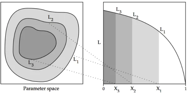
Figure 1.11 For an arbitrary paramteter space samples are sorted by amount of enclosed prior mass X. This by construction also sorts the samples in terms of increasing likelihood. Figure reproduced from [219]

where dX ≡π(~θ)d~θ is a mass element associated with the prior PDF π(~θ). This can in turn be used to evaluate the equivalent mass element for a posterior PDF

p(~θ) as

dP =p(~θ)d~θ= L(

~

θ)π(~θ)d~θ

Z (1.31)

For a high-dimensional parameter space the evaluation of the integral in Equa-tion 1.30 will be very computationally expensive, but through the recasting of the integral in terms of dX and defining the cumulative prior mass, containing all likelihood values greater than λ, as

X(λ) =

Z

L(~θ)>λ

π(θ~)d~θ (1.32)

it has been reduced to a much simpler monotonically increasing function taking values in the range X(0) = 1 to X(∞) = 0. By finding the inverse of Equa-tion 1.32,L(X(λ)) =λ, the evidence as given byEquation 1.30 becomes

Z =

Z 1

0

where as shown in Figure 1.11 the integrand L(X) is always positive and de-creasing. Dividing the prior mass X into small elements, as required in the transformation from ~θ, then allows the prior mass to be sorted according to in-creasing likelihood within each prior mass element which allows for the integral in Equation 1.33 to be represented as a weighted sum over these mass elements. As increasing X by construction gives decreasing L(X) it is then possible to put bounds on the evidence as

m X i=0 Li(Xi−Xi+1)≤Z ≤ m X i=1 Li(Xi−1−Xi) +LmaxXm (1.34)

for a set of m prior mass elements and the highest likelihood point in this set given by Lmax. The highest computational expense within a nested sampling

method would be the sorting of the prior mass elements, but through the record of previous samples, and their associated likelihood values, it is possible to sidestep the sorting altogether by only accepting samples with L(X)> Li−1.

For the nested sampling implementation used for CBC parameter estimation [248, 11, 247] the algorithm is initialised by stochastically sprinkling a prede-termined number of samples called live points, using a MCMC (as described in

subsubsection 1.3.2.1), following the defined prior PDF. After sorting the samples according to prior mass, or likelihood, the lowest likelihood sample is removed from the set of live points and a new sample is drawn from the prior distribution. As shown in Figure 1.12 samples are only accepted into the set of live points if their likelihoods are higher than the bound set by the new lowest likelihood. The condition for termination can be either set to a predetermined number of steps or more often when any additional sample would be unable to increase the evidence by a predefined small fraction (given as the width of the bounds fromEquation 1.34). After termination the collection of discarded live points are reweighted according to their individual prior and likelihood values, combined with the global evidence, to produce a set of posterior samples. There are also extensions to nested sampling where the prior volumes are divided into smaller regions for improved efficiency for sampling highly multi-modal PDFs [c.f. Multi-Nest 89, 97].

Figure 1.12 For an example analysis containing three live points it is clear how the sample enclosing the highest prior massX, and representing the lowest likelihood, is replaced in each step by a higher likelihood point. After five steps the nested sampling is terminated, leaving in total eight samples distributed according to the likelihood PDF with a higher sample density at higher likelihoods. Figure reproduced from [219]

by construction an evidence is computed, therefore encouraging use of model se-lection approaches through Bayes factors. It has however been shown in multiple studies [11, 247, 232] that both samplers show a high level of agreement, and thus are both able to efficiently produce a set of samples which are an accurate representation of the posterior distribution under investigation

1.4

Structure of Thesis

1.4.1

Chapter 2

Chapter 2focuses on the role of post-Newtonian dynamics in the formation and evolution of compact binary black holes which includes an intermediate mass black hole.

This chapter is adapted from a paper in preparation by Carl-Johan Haster, Fabio Antonini, Ilya Mandel and Vicky Kalogera [108]. This paper grew out of a collaboration between the four authors during my pre-doctoral fellowship at the Center for Interdisciplinary Exploration in Astrophysics at Northwestern Univer-sity. My contribution to this work was (i) initialised, ran and post-processed the N-body of the 12 cluster models, (ii) lead the analysis of the results of the IMBH–BH dynamics (iii) wrote the paper. The remainder of this subsection is adapted from the abstract of this paper.

The intermediate mass-ratio inspiral of a stellar compact remnant into an intermediate mass black hole (IMBH) can produce a gravitational wave (GW) signal that is potentially detectable by current ground-based GW detectors (e.g., Advanced LIGO) as well as by planned space-based interferometers (e.g., eLISA). Here, we present results from direct integration of the post-Newtonian N-body equations of motion describing stellar clusters containing an IMBH and a popu-lation of stellar black holes (BHs) and solar mass stars. We take particular care to simulate the dynamics closest to the IMBH, including post-Newtonian effects up to order 2.5. Our simulations show that the IMBH readily forms a binary with a BH companion. This binary is gradually hardened by transient 3-body or 4-body encounters, leading to frequent substitutions of the BH companion, while the binary’s eccentricity experiences large amplitude oscillations due to the

Lidov-Kozai resonance. We also demonstrate suppression of these resonances by the relativistic precession of the binary orbit. We find an intermediate mass-ratio inspiral in one of the 12 cluster models we evolved for ∼ 100 Myr. This cluster hosts a 100M IMBH embedded in a population of 32 10M BH and 32,000 1M stars. At the end of the simulation, after ∼ 100 Myr of evolution, the

IMBH merges with a BH companion. The IMBH-BH binary inspiral starts in the eLISA frequency window (_& 1mHz) when the binary reaches an eccentricity 1−e'10−3. After'105 _{years the binary moves into the LIGO frequency band}

with a negligible eccentricity. We comment on the implications for GW searches, with a possible detection within the next decade.

1.4.2

Chapter 3

Chapter 3 consists of a parameter estimation study on intermediate mass ratio coalescences, like the binary formed in the study described in chapter 2.

This chapter is adapted from a paper by Carl-Johan Haster, Zhilu Wang, Christopher P. L. Berry, Simon Stevenson, John Veitch and Ilya Mandel. My contribution to this work was to (i) design the initial parameters of this study,

(ii) aid Zhilu Wang (a summer student in the group) to run the simulations,

(iii) lead the post-processing and collating of the results, (iv) write the paper. This paper is published in MNRAS [110] and has arXiv number 1511.01431. The remainder of this subsection is adapted from the abstract of this paper.

Gravitational waves from coalescences of neutron stars or stellar-mass black holes into intermediate-mass black holes (IMBHs) of_&100 solar masses represent one of the exciting possible sources for advanced gravitational-wave detectors. These sources can provide definitive evidence for the existence of IMBHs, probe globular-cluster dynamics, and potentially serve as tests of general relativity. We analyse the accuracy with which we can measure the masses and spins of the IMBH and its companion in intermediate-mass ratio coalescences. We find that we can identify an IMBH with a mass above 100 M with 95% confidence

provided the massive body exceeds 130 M. For source masses above ∼200 M,

the best measured parameter is the frequency of the quasi-normal ringdown. Consequently, the total mass is measured better than the chirp mass for massive

binaries, but the total mass is still partly degenerate with spin, which cannot be accurately measured. Low-frequency detector sensitivity is particularly important for massive sources, since sensitivity to the inspiral phase is critical for measuring the mass of the stellar-mass companion. We show that we can accurately infer source parameters for cosmologically redshifted signals by applying appropriate corrections. We investigate the impact of uncertainty in the model gravitational waveforms and conclude that our main results are likely robust to systematics.

1.4.3

Chapter 4

Chapter 4 presents an accurate and computationally efficient method for param-eter estimation of CBC signals.

This chapter is adapted from a paper byCarl-Johan Haster, Ilya Mandel and Will M. Farr. My contribution to this work was to (i) design and write the software used in this study, (ii) run simulations, (iii) verify the results, focusing on the accuracy of the recovered credible regions, against alternative methods,

(iv) write the paper. This paper is published in Classical and Quantum Gravity [109] and has arXiv number 1502.05407. The remainder of this subsection is adapted from the abstract of this paper.

In many previous studies, predictions for the accuracy of inference on

gravitational-wave signals relied on computationally inexpensive but often impre-cise techniques. Recently, the approach has shifted to actual inference on noisy signals with complex stochastic Bayesian methods, at the expense of significant computational cost. Here, we argue that it is often possible to have the best of both worlds: a Bayesian approach that incorporates prior information and correctly marginalizes over uninteresting parameters, providing accurate poste-rior probability distribution functions, but carried out on a simple grid at a low computational cost, comparable to the inexpensive predictive techniques.

Chapter 2

N

−

body dynamics of

Intermediate mass ratio inspirals

This chapter is adapted from a paper in preparation byCarl-Johan Haster, Fabio Antonini, Ilya Mandel and Vicky Kalogera [108]. This paper grew out of a collab-oration between the four authors during my pre-doctoral fellowship at the Center for Interdisciplinary Exploration in Astrophysics at Northwestern University. My contribution to this work was (i)initialised, ran and post-processed the N-body of the 12 cluster models, (ii) lead the analysis of the results of the IMBH–BH dynamics (iii) wrote the paper.

2.1

Introduction

Intermediate mass black holes (IMBHs) are conjectured to occupy the mass range between stellar-mass black holes (BHs), with masses_.100M, and supermassive black holes with masses _& 106M [see 165, for a review]. While the existence of some IMBH candidates in dwarf spheroidal galaxies has been conjectured by extending theM–σrelation [99] [but see145], dynamical measurements of IMBHs in the few-hundred solar-mass range are extremely challenging [e.g., 183]. The best evidence for such lower mass IMBHs (with mass ∼ 100M) could come from ultraluminous X-ray sources [but see 49]; for example, [182] have claimed a mass of ∼400 M for M82 X-1 from quasi-periodic oscillations, while a mass

around 104_{M has been suggested for the brightest ultraluminous X-ray source}

HLX-1 [e.g.,86,74,95], but these dynamical measurements alone can not provide conclusive proof for the existence of IMBHs.

If these lower-mass IMBHs reside in globular clusters, they will play an impor-tant role in cluster dynamics [e.g.237,240,128,134,146]. Of particular interest to our study is the likely tendency of IMBHs to dynamically form compact binaries with other compact remnants [e.g.224,163, 166, 32, 58,151,35,156,155]. Gen-erally, these analyses find that the IMBH readily captures a binary companion. The binary is subsequently hardened through a sequence of 3-body and 4-body interactions, occasionally with substitutions which make a black hole (BH) of a few tens of solar masses the most likely IMBH companion, and possible Lidov-Kozai (LK) resonances [135, 129] if hierarchical triples are formed. Eventually, the IMBH-BH binary merges through the radiation of gravitational waves, emit-ting a signal that is potentially detectable by the Advanced LIGO ground-based GW detectors [106, 17,220, 110].

Previous simulations of globular clusters with IMBH coalescences have gen-erally simplified the interactions in order to avoid excessive computational cost. For example, Gültekin et al. [100] considered a series of individual Newtonian interactions interspersed with orbital evolution through GW emission. Mandel et al. [151] carried out analytical estimates of the hardening sequence to obtain the intermediate mass-ratio merger timescale. Leigh et al. [134] simulated the entire cluster with a mixture of analytical and numerical N-body analytical cal-culations, while MacLeod et al. [146] focused theirN-body investigation on tidal disruptions of stars by the IMBH as well as merger events. We note that in the previous literature effects of pN terms are either not accounted for [134], or included only at the 2.5pN level [204, 146]. In this chapter we show a clear ex-ample in which lower order pN terms play a fundamental role in the dynamics. More specifically, an essential element that differs between the relativistic and non-relativistic dynamics turns out to be the 1pN precession of the periapsis.

We introduce our numerical method and the simulation setup in section 2.2. We describe our simulation results insection 2.3. We discuss the results, including the detectability of GWs from intermediate mass-ratio coalescences, insection 2.4.

2.2

Simulations

The N-body systems considered here consist of a massive particle, representing an IMBH, and two additional lower-mass species representing 10M compact

remnants and 1M stars. Integrations of the N-body equations of motion were carried out using the direct summation N-body code phiGRAPEch [105]. This code incorporates Mikkola’s algorithmic chain regularization scheme including post-Newtonian terms of order 1pN, 2pN and 2.5pN [AR-CHAIN, 162]. Velocity dependent forces were included using the generalized midpoint method described by Mikkola and Merritt [161]. The algorithm produces exact trajectories for Newtonian two-body motion and regular results for strong encounters involving arbitrary numbers of bodies. Particles moving beyond the “chain radius” (rchain)

were advanced using a fourth-order integrator with forces computed on GPUs using the Sapporo library [92]. The chain particles were influenced by the global cluster dynamics through the particles in a perturber region, within a radius

rperturb from the IMBH. phiGRAPEch is an ideal tool for the study of the

dy-namics of IMBHs in star clusters because it allows to study with extremely high precision the joint effect of 1pN, 2pN and 2.5pN terms and their interplay with Newtonian perturbations to the motion.

We performed 12 simulations all initialized as a King model with no primordial binaries, containing two mass species (BHs and stars) with a relative mass ratio of 10 : 1, and assuming that the total mass in BHs is 1% of the total cluster mass. Finally, an initially stationary IMBH was placed at the center of the cluster. The analytical King model where chosen because, despite of their dynamical simplicity, they provide a good fit to observed surface brightness profiles. King models are defined as approximate iso-thermal spheres (where the velocity of a particle is largely independent of its position in the cluster) with a modified density profile such that the energy, as well as the number density, decreases with radius until it becomes zero at the tidal radiusrt. Together with the King radius

r0 ≡

s

9σ2

4πGρ0

(2.1) where σ is the velocity dispersion of the cluster and ρ0 is its central density, this

defines the concentration parameter W0 ≡rt/r0 (W0 = 7 for all our simulations).

The simulations were performed with number of particles N ⊂ {32768,65536}

IMBH mass, M ⊂ {50,100,200}M and cluster virial radius rv defined as

M2 tot rv ≡ N X i=0 N X j6=i mimj |~ri−~rj| (2.2)

given cluster total massMtot, and particle masses and distancesmand~rsummed over all particle pairs i, j. rv was in these simulations set as 3.5 pc which in turn

gave rv ∼5r0 for our choice of King models. For N = 32768 and all three IMBH

masses, simulations with rv ⊂ {0.35,1.0} pc were also performed. The inclusion

of high-order pN terms fixes the physical scale of the cluster, thus removing the conventional freedom for rescaling simulations in cluster size and density.

We observe the IMBH forming a binary with a BH within _.20Myr in every simulated cluster. Only in one cluster (N = 32768, M = 100M, rv = 3.5pc) we

observe a merger within the simulated time ('100Myr), and in what follows we will focus on describing the detailed dynamics of this cluster. We acknowledge that as the main focus of this study is the dynamical formation and evolution of binaries, and higher order N-tuples, with the IMBH as the primary companion, all cluster particles are solely characterized by their mass and no stellar evolution is included in these simulations.

2.3

Results

The simulated globular cluster was initialised with the IMBH at rest at the center while the remaining stars and BHs follows a King model. Figure 2.1 shows the position of the IMBH and a subset of BH particles, and their subsequent move-ment within the cluster, relative to the center of mass of the entire cluster. This subset of the BH population were those that were ejected from the cluster during the simulation. Although the IMBH is initially at rest at the cluster center of mass, it quickly experiences significant Brownian motion within a sphere of radius

∼0.1pc around the center of mass. The typical distance wandered by the IMBH in the core is larger than the radius of influence of the IMBH.

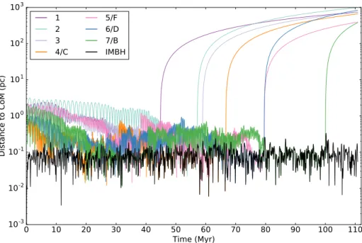
0 10 20 30 40 50 60 70 80 90 100 110 Time (Myr) 10-3 10-2 10-1 100 101 102 103 Distance to CoM (pc) 1 2 3 4/C 5/F 6/D 7/B IMBH

Figure 2.1 Time evolution of the distance of the IMBH (in black) to the center of mass (CoM) of the entire cluster. Note how the IMBH is wandering throughout the simulation within a central region of extent _.0.1pc around the cluster CoM. Also shown (in colour) are the BHs that were ejected from the cluster and the corresponding time of ejection. BHs for which we have assigned both a numerical and alphabetical index were bound to the IMBH before being ejected from the cluster. The evolution of the orbits of these BHs are also shown in Figure 2.2.

Shifting the focus from the global dynamical behaviour within the cluster,

Figure 2.2 displays the time evolution of the relative distance to the IMBH of those BHs which experienced close encounters with the IMBH at some point of the simulation. In this figure we see that while the IMBH is interacting only weakly with its surroundings at the start of the simulation, after∼3 Myrs it forms a wide binary with a stellar particle, and after ∼ 25 Myrs the binary companions are BHs, consistent with the expected mass segregation in this cluster. By comparing the ejected BHs between Figure 2.1 and Figure 2.2 it is clear that after the first few ejected BHs (which were driven by their initially relatively high kinetic energy and interactions with other cluster members) and following the formation of the IMBH-BH binary, all subsequent ejections are driven by interactions with the IMBH-BH binary. These interactions lead to the frequent substitution of the IMBH binary companion, with three out of the five observed substitution events