Statistics Preprints
Statistics
1-12-2018
Predictive mean matching imputation in survey
sampling
Shu Yang
Jae Kwang Kim
Iowa State University, [email protected]
Follow this and additional works at:
https://lib.dr.iastate.edu/stat_las_preprints
Part of the
Design of Experiments and Sample Surveys Commons
This Article is brought to you for free and open access by the Statistics at Iowa State University Digital Repository. It has been accepted for inclusion in Statistics Preprints by an authorized administrator of Iowa State University Digital Repository. For more information, please contact
Recommended Citation
Yang, Shu and Kim, Jae Kwang, "Predictive mean matching imputation in survey sampling" (2018).Statistics Preprints. 139. https://lib.dr.iastate.edu/stat_las_preprints/139
Predictive mean matching imputation in survey sampling
AbstractPredictive mean matching imputation is popular for handling item nonresponse in survey sampling. In this article, we study the asymptotic properties of the predictive mean matching estimator of the pop- ulation mean. For variance estimation, the conventional bootstrap inference for matching estimators with fixed matches has been shown to be invalid due to the nonsmoothness nature of the matching estimator. We propose asymptotically valid replication variance estimation. The key strategy is to construct repli- cates of the estimator directly based on linear terms, instead of individual records of variables. Extension to nearest neighbor imputation is also discussed. A simulation study confirms that the new procedure provides valid variance estimation.
Keywords
Bootstrap, Jackknife variance estimation, Martingale central limit theorem, Missing at random Disciplines
Design of Experiments and Sample Surveys | Statistics and Probability Comments
This is a pre-print made available through arxiv:https://arxiv.org/abs/1703.10256.
arXiv:1703.10256v3 [stat.ME] 12 Jan 2018
Predictive mean matching imputation in survey sampling
Shu Yang Jae Kwang Kim
Abstract
Predictive mean matching imputation is popular for handling item nonresponse in survey sampling. In this article, we study the asymptotic properties of the predictive mean matching estimator of the pop-ulation mean. For variance estimation, the conventional bootstrap inference for matching estimators with fixed matches has been shown to be invalid due to the nonsmoothness nature of the matching estimator. We propose asymptotically valid replication variance estimation. The key strategy is to construct repli-cates of the estimator directly based on linear terms, instead of individual records of variables. Extension to nearest neighbor imputation is also discussed. A simulation study confirms that the new procedure provides valid variance estimation.
Key Words: Bootstrap; Jackknife variance estimation; Martingale central limit theorem; Missing at random.
1. Introduction
Predictive mean matching imputation (Rubin; 1986; Little; 1988) is popular for handling item nonresponse in survey sampling. Hot deck imputation within imputation cells is a special case, where the predictive mean function is constant within cells. On the other hand, predictive mean matching is a version of nearest neighbor imputation. In nearest neighbor imputation, the vector of the auxiliary variablesxis directly used in determining the nearest neighbor, while in predictive mean matching imputation, a scalar predictive mean function is used in determining the nearest neighbor. The nearest neighbor is then used as a donor for hot deck imputation.
Although these imputation methods have a long history of application, there are relatively few papers on investigating their asymptotic properties. Kim et al. (2011) presented an application of nearest neighbor imputation for the US census long form data. Vink et al. (2014) and Morris et al. (2014) investigated using predictive mean matching as a tool for multiple imputation via simulation studies. Chen and Shao
(2000, 2001) have developed a nice set of asymptotic theories for the nearest neighbor imputation estimator. In econometrics, Abadie and Imbens (2006, 2008, 2011, 2016) studied the matching estimator for causal
effect estimation from observational studies. Up to our best knowledge, there is no literature on theoretical investigation ofestimated predictive mean matchingfor mean estimation in survey sampling, which motivates this article.
Predictive mean matching is implemented in two steps. First, the predictive mean function is estimated. Second, for each nonrespondent, the nearest neighbor is identified among the respondents based on the
predictive mean function, and then the observed outcome value of the nearest neighbor is used for imputation. Because the predictive mean function is estimated prior to matching, it is necessary to account for the uncertainty due to parameter estimation. Because of the non-smooth nature of matching, our derivation is based on the technique developed by Andreou and Werker (2012), which offers a general approach for deriving the limiting distribution of statistics that involve estimated nuisance parameters. This technique
has been successfully used in Abadie and Imbens (2016) for the matching estimators of the average causal effects based on the estimated propensity score. We extend their results to the matching estimator in the
survey sampling context. In addition, we establish robustness of the predictive mean matching estimator which is consistent if the mean function satisfies a certain Lipschitz continuity condition.
Lack of smoothness also makes the conventional replication methods invalid for variance estimation for the predictive mean matching estimator. Abadie and Imbens (2008) demonstrated the failure of the bootstrap for matching estimators with a fixed number of matches. We propose new replication variance estimation
for the predictive mean matching estimator in survey sampling. Based on the martingale representation of the predictive mean matching estimator, we construct replicates of the estimator directly based on its linear terms. In this way, the distribution of the number of times that each unit is used as a match can be preserved, which leads to a valid variance estimation. Furthermore, our replication variance method is flexible and can accommodate bootstrap, jackknife, among others.
The rest of this paper is organized as follows. In Section 2, we introduce the basic set-up in the context of survey data and the predictive mean matching procedure. In Section 3, we establish and compare the asymptotic distributions of the predictive mean matching estimator when the predictive mean function is known or is estimated. In Section 4, we propose the new replication variance estimators and establish their consistency. In Section 5, we evaluate the finite sample performance of the proposed estimators via a
simulation study. We end with a brief discussion in Section 6. All proofs are deferred to the Appendix.
2. Basic Set-up
LetFN ={(xi, yi, δi) :i= 1, . . . , N} denote a finite population, wherexi is always observed,yi has missing
values, andδi is the response indicator of yi, i.e., δi = 1 ifyi is observed and 0 if it is missing. Theδi’s are
defined throughout the finite population, as in Fay (1992), Shao and Steel (1999), and Kim et al. (2006). We assume thatFN is a random sample from a superpopulation modelζ, andN is known. Our objective is
to estimate the finite population meanµ=N−1PN
i=1yi. Let A denote an index set of the sample selected
by a probability sampling design. Let Ii be the sampling indicator, i.e., Ii = 1 if unit i is selected into
throughout the sample. We make the following assumption for the missing data process.
Assumption 1 (Missing at random and positivity) The missing data process satisfiespr(δ = 1|x, y) = pr(δ = 1|x), which is denoted byp(x), and with probability 1, p(x)> ǫfor a constant ǫ >0.
In order to construct the imputed values, we assume that
E(yi|xi) =m(xi;β∗), (1)
holds for every unit in the population, wherem(·) is a function ofx known up toβ∗. Under Assumption 1,
let the normalized estimating equation forβ be
SN(β) = n1/2 N X i∈A 1 πi δig(xi;β){yi−m(xi;β)}= 0, (2)
whereg(x;β) is any function with which the solution to (2) exists uniquely. To simply the presentation, let
g(x;β) be ˙m(x;β) = ∂m(x;β)/∂β. General functions g(x;β) can be considered at the expense of heavier notation. Under certain regularity conditions (e.g. Fuller; 2009, Ch. 2), the solution ˆβ converges to β∗ in
probability. Here, the probability distribution is the joint distribution of the sampling distribution and the superpopulation model (1). The sampling weight π−1
i is used to obtain a consistent estimator of β ∗
even under informative sampling (Berg et al.; 2016).
Under the model (1), the predictive mean matchingmethod can be described as follows:
Step 1. Obtain a consistent estimator ofβ, denoted by ˆβ, by solving (2). For each unitiwithδi= 0, obtain
a predicted value of yi as ˆmi =m(xi; ˆβ). Find the nearest neighbor of unit i from the respondents
with the minimum distance between ˆmj and ˆmi. Leti(1) be the index of the nearest neighbor of unit
i, which satisfies d( ˆmi(1),mˆi)≤d( ˆmj,mˆi), for anyj ∈ AR ={i∈ A:δi = 1}, whered(·,·) denotes a
generic distance function, e.g., d(mi, mj) =|mi−mj|for scalarmi and mj.
Step 2. The imputation estimator based on predictive mean matchingis computed by
ˆ µPMM= 1 N X i∈A 1 πi δiyi+ (1−δi)yi(1) . (3)
In (3), the imputed values are real observations. The imputation model is used only for identifying the nearest neighbor, but not for creating the imputed values. Variance estimation of ˆµPMM is challenging
because of the nonsmoothness of the matching mechanism in Step 1. In the next section, we formally discuss the asymptotic properties of the predictive mean matching estimator.
3. Main Result
3.1 Predictive mean matching
We introduce additional notation. LetA = AR∪AM, where AR and AM are the sets of respondents and
nonrespondents, respectively. Definedij = 1 ifyj(1)=yi, i.e., unitiis used as a donor for unitj∈AM, and
dij = 0 otherwise. We write ˆµPMM= ˆµPMM( ˆβ), where
ˆ µPMM(β) = 1 N X i∈A 1 πi {δiyi+ (1−δi)yi(1)} = 1 N X i∈A 1 πi δiyi+ X j∈A 1−δj πj X i∈A δidijyi = 1 N X i∈A δi πi (1 +kβ,i)yi, (4) with kβ,i= X j∈A πi πj (1−δj)dij. (5)
Under simple random sampling, kβ,i = Pj∈A(1−δj)dij is the number of times that unit i is used as the
nearest neighbor for nonrespondents, where determination of the nearest neighbor is based on the predictive mean functionm(xi;β).
We first consider the case whenβ∗
, and hencem(xi) =m(xi;β∗), is known. Suppose that the
superpop-ulation model satisfies the following assumption.
Assumption 2 (i) The matching variable m(x)has a compact and convex support, with its density bounded and bounded away from zero. Denote mi = m(xi). Let g1(mi) and g0(mi) be the conditional density
of mi given δi = 1 and δi = 0, respectively. Suppose that there exist constants C1L and C1U such that
C1L≤g1(mi)/g0(mi)≤C1U; (ii) there existsδ >0 such that E(|y|2+δ|x) is uniformly bounded for any x.
Assumption 2 (i) is a convenient regularity condition (Abadie and Imbens; 2006). Assumption 2 (ii) is a moment condition for establishing the central limit theorem.
Denote Ep(·) and varp(·) to be the expectation and the variance under the sampling design, respectively.
We impose the following regularity conditions on the sampling design.
Assumption 3 (i) There exist positive constantsC1 andC2 such that C1 ≤πiN n−1≤C2,fori= 1, . . . , N;
(ii) nN−1 = o(1); (iii) the sequence of the Hotvitz-Thompson estimators µˆ
HT = N−1Pi∈Aπ −1
i yi satisfies
Assumption 3 is a widely accepted assumption in survey sampling (Fuller; 2009, Ch. 1).
To study the asymptotic properties of the predictive mean matching estimator, we use the following decomposition: n1/2{µˆPMM(β)−µ}=DN(β) +BN(β), (6) where DN(β) = n1/2 N X i∈A 1 πi [m(xi;β) +δi(1 +kβ,i){yi−m(xi;β}]−µ ! , (7) and BN(β) = n1/2 N X i∈A 1 πi (1−δi){m(xi(1);β)−m(xi;β)}. (8) The difference m(xi(1);β∗)−m(x
i;β∗) accounts for the matching discrepancy, and BN(β∗) contributes to
the asymptotic bias of the matching estimator. In general, if the matching variable x is p-dimensional, Abadie and Imbens (2006) showed thatd(xi(1), xi) =Op(n−1/p). Therefore, for nearest neighbor imputation
withp≥2, the biasBN(β∗) =Op(n1/2−1/p)6=op(1) is not negligible; whereas, for predictive mean matching,
the matching variable is a scalar functionm(x), and henceBN(β∗) =Op(n−1/2) =op(1). We establish the
asymptotic distribution of ˆµPMM(β∗).
Theorem 1 Under Assumptions 1–3, suppose that m(x) = E(y | x) = m(x;β∗
) and σ2(x) = var(y | x). Then,n1/2{µˆ PMM(β∗)−µ} → N(0, V1) in distribution, asn→ ∞, where V1=Vm+Ve (9) with Vm = lim n→∞nN −2E[var p{ X i∈A π−1 i m(xi)}], Ve = lim n→∞nN −2E{ N X i=1 π−1 i (1−πi)δi(1 +kβ∗,i)2σ2(xi)}, andkβ,i is defined in (5).
In practice,β∗is unknown and therefore has to be estimated prior to matching. Following Abadie and Imbens
(2016),the following theorem presents the approximate asymptotic distribution of ˆµPMM( ˆβ).
Theorem 2 Under Assumptions 1–3 and certain regularity conditions specified in the Appendix,n1/2{µˆ
PMM( ˆβ)−
µ} → N(0, V2) in distribution, asn→ ∞, where βˆ is the solution to the estimating equation (2) and
V2=V1−γ1TV −1 s γ1+γ2T τ−1 β∗Vsτ −1 β∗ γ2, (10) γ1 = limn→∞nN −2E{PN i=1π −1 i (1−πi)δi(1 +kβ∗,i)g(xi;β∗)σ2(xi)}, γ2=E{m˙(x;β∗)},V1 is defined in (9), Vs= var{SN(β∗)}, τβ =E{p(x) ˙m(x;β) ˙m(x;β)T}, and p(x) = pr(δ = 1|x).
The difference between V2 andV1,−γ1TV −1 s γ1+γ2T(τ −1 β∗Vsτ −1
β∗)γ2, can be positive or negative. Thus, the
estimation error in the predictive mean function should not be ignored. This is different from the result in Abadie and Imbens (2016) that matching on the estimated propensity score always improves the estimation efficiency when matching on the true propensity score. To explain the difference, we note that the propensity score is auxiliary for estimating the population mean of outcome; whereas the predictive mean function is
not.
3.2 Nearest neighbor imputation
Nearest neighbor imputation can be described in the following steps:
Step 1. For each unit i with δi = 0, find the nearest neighbor from the respondents with the
mini-mum distance between xj and xi. Let i(1) be the index set of its nearest neighbor, which satisfies
d(xi(1), xi)≤d(xj, xi),forj∈AR.
Step 2. The nearest neighbor imputation estimator of µis computed by ˆ µNNI= 1 N X i∈A 1 πi δiyi+ (1−δi)yi(1) = 1 N X i∈A 1 πi δi(1 +ki)yi, (11)
where ki is defined similarly as in (5), but with the matching variablex.
Following (6), writen1/2(ˆµNNI−µ) =DN+BN,where
DN =n1/2 1 N X i∈A 1 πi [m(xi) +δi(1 +ki){yi−m(xi)}]−µ ! , and BN = n 1/2 N X i∈A 1 πi (1−δi){m(xi(1))−m(xi)}. (12)
Because the matching is based on ap-vector matching variable, the bias termBN =Op(n1/2−1/p) withp≥2
is not negligible. For bias correction, let ˆm(x) be a consistent estimator of m(x) = E(y | x). Then, we can estimate BN by ˆBN =n−1/2NPi∈Aπ
−1
i (1−δi){mˆ(xi(1))−mˆ(xi)}.A bias-corrected nearest neighbor
imputation estimator of µis ˜ µNNI= 1 N X i∈A 1 πi {δiyi+ (1−δi)yi∗}, (13) where y∗
i = ˆm(xi) +yi(1)−mˆ(xi(1)). Under certain regularity conditions imposed on the nonparametric
estimator ˆm(x), ˆBN is consistent forBN, i.e., ˆBN −BN =op(1).Then, the bias-corrected nearest neighbor
imputation estimator has the same limiting distribution as the predictive mean matching estimator with knownβ∗ has.
3.3 Robustness against the predictive mean function specification
To discuss the robustness of the predictive mean matching estimator against the predictive mean function specification, letm(x;β) be a working model forE(y|x), ˆβ be the estimator of β solving (2), andβ∗ be its
probability limit. We also use m =m(x;β∗
) for shorthand. We require the following assumption hold for the working model.
Assumption 4 E(y |m) is is Lipschitz continuous in m; i.e., there exists a constant C3 such that |E(y |
mi)−E(y|mj)| ≤C3|mi−mj|, for any i, j.
Assumption 4 is trivial whenm(x;β) is correctly specified forE(y|x), because in this caseE(y|m) =m.
Theorem 3 Under Assumptions 1–4, the predictive mean matching estimator based on the working model
m(x;β∗
) is consistent for µ.
The result can be obtained directly from the decomposition (6) by replacing m(x;β) in DN(β) and
BN(β) with E{y |m(x;β)}. The new term DN(β∗) is still consistent for zero; by Assumption 4, the new
bias term becomes
|BN(β∗)| = | n1/2 N X i∈A 1 πi (1−δi) E{y|m(xi(1);β∗)} −E{y|m(xi(1);β∗)} | ≤ n 1/2 N C3 X i∈A 1 πi (1−δi)|m(xi(1);β∗)−m(xi;β∗)|=Op(n−1/2).
4. Replication Variance Estimation
We consider replication variance estimation (Rust and Rao; 1996; Wolter; 2007) for the predictive mean matching estimator. Let ˆµ be the Horvitz-Thompson estimator ofµ. The replication variance estimator of ˆ
µtakes the form of
ˆ Vrep(ˆµ) = L X k=1 ck(ˆµ(k)−µˆ)2, (14)
where L is the number of replicates, ck is the kth replication factor, and ˆµ(k) is the kth replicate of ˆµ.
When ˆµ=P
i∈Aωiyi, we can write the replicate of ˆµas ˆµ
(k) =P
i∈Aω
(k)
i yi with some ω(ik) fori∈A. The
replications are constructed such that E{Vˆrep(ˆµ)} = var(ˆµ){1 +o(1)}. For example, in delete-1 jackknife
under probability proportional to size sampling with ωi = N−1π−i 1, we have L = n, ck = (n−1)/n, and
ω(ik) =nωi/(n−1) ifi6=k, and ω(kk)= 0.
We propose a new replication variance estimation for the predictive mean matching estimator. We first consider ˆµPMM(β∗) with a known β∗ given in (4). For simplicity, we suppress the dependence of
quantities on β∗
. Write ˆµPMM−µ = (ˆµPMM−ψˆHT) + ( ˆψHT−µψ) + (µψ −µ), where ˆψHT = Pi∈Aωiψi,
ψi = m(xi) + δi(1 +ki){yi −m(xi)}, µψ = N−1PNi=1ψi. By Theorem 1, µPMM−ψˆHT = op(n−1/2).
Together with the fact that µψ −µ =Op(N−1/2) and nN−1 = o(1), ˆµPMM−µ = ˆψHT−µψ +op(n−1/2).
Therefore, with negligible sampling fractions, it is sufficient to estimate the variance of ˆψHT−µψ. Because
Ep( ˆψHT−µψ) = 0, we have var( ˆψHT−µψ) =E{varp( ˆψHT−µψ)},which is essentially the sampling variance
of ˆψHT. This suggests that we can treat {ψi : i ∈ A} as pseudo observations in applying the replication
variance estimator. Otsu and Rai (2016) used a similar idea to develop a wild bootstrap technique for a matching estimator. To be specific, we construct replicates of ˆψHT as follows: ˆψHT(k) = Pi∈Aω
(k)
i ψi,
where ω(ik) is the replication weight that account for complex sampling design. The replication variance estimator of ˆψHT is obtained by applying ˆVrep(·) in (14) for the above replicates ˆψ(HTk). It follows that
E{Vˆrep( ˆψHT)}= var( ˆψHT−µψ){1 +o(1)}= var(ˆµPMM−µ){1 +o(1)}.
We now consider ˆµPMM( ˆβ), which can be expressed as ˆµPMM( ˆβ) =Pi∈Aωi[m(xi; ˆβ) +δi(1 +kβ,iˆ ){yi−
m(xi; ˆβ)}] +op(n−1/2).To compute the replicates of ˆµPMM( ˆβ), we propose two steps:
Step 1. Obtain the kth replicate of ˆβ, denoted as ˆβ(k), by solving SN(k)(β) = P
i∈Aω
(k)
i δi ×g(xi;β){yi −
m(xi;β)}= 0.
Step 2. Obtain the kth replicate as ˆ µ(PMMk) ( ˆβ(k)) =X i∈A ωi(k)[m(xi; ˆβ(k)) +δi(1 +kβˆ(k) ,i){yi−m(xi; ˆβ (k))}]. (15)
Ifβ∗ is known, we do not need to reflect the effect of estimatingβ∗, and the above procedure with two steps
reduces to the one we proposed for the case when β∗ is known. On the other hand, when β∗ is estimated,
Step 1 is necessary, because as shown in Theorem 2, the predictive mean matching estimators by matching on the true and estimated predictive mean function may have different asymptotic distributions.
The consistency of the replication variance estimator is presented in the following theorem.
Theorem 4 Under the assumptions in Theorem 2, suppose that Vˆrep(ˆµ) in (14) is consistent for varp(ˆµ).
Then, ifnN−1=o(1), the replication variance estimators forµˆ
PMM( ˆβ)is consistent, i.e.,nVˆrep{µˆPMM( ˆβ)}/V2→
1 in probability, asn→ ∞, where the replicates of µˆPMM( ˆβ) are given in (15), and V2 is given in (10).
5. A Simulation Study
In this simulation study, we investigate the performance of the proposed replication variance estimator. For generating finite populations of sizeN = 50,000: first, letx1i,x2i andx3i be generated independently from
as (P1)yi =−1 +x1i+x2i+ei, (P2) yi =−1.167 +x1i+x2i+ (x1i −0.5)2 + (x2i −0.5)2 +ei, and (P3)
yi = −1.5 +x1i +· · ·+x6i+ei. The covariates are fully observed, but yi is not. The response indicator
of yi, δi, is generated from Bernoulli(pi) with logit{p(xi)} = 0.2 +x1i +x2i. This results in the average
response rate about 75%. The parameter of interest isµ=N−1PN
i=1yi. To generate samples, we consider
two sampling designs: (S1) simple random sampling with n = 400; (S2) probability proportional to size sampling. In (S2), for each unit in the population, we generate a size variablesi as log(|yi+νi|+ 4), where
νi ∼ N(0,1). The selection probability is specified as πi = 400si/PNi=1si. Therefore, (S2) is informative,
where units with larger yi values have larger probabilities to be selected into the sample.
For estimation, we consider predictive mean matching imputation, nearest neighbor imputation, and stochastic regression imputation. In stochastic regression imputation, for units with δi= 0, the imputation
of yi is obtained as yi∗ = ˆyi + ˆe∗i, where ˆyi = m(xi; ˆβ) and ˆe∗i is randomly selected from the observed
residuals {ˆei = yi −yˆi : δi = 1}. For (P1) and (P2), we specify the predictive mean function to be
m(x;β) =β0+β1x1+β2x2. Note that for (P1),m(x;β) is correctly specified; whereas for (P2),m(x;β) is
misspecified. For (P3), we specify the mean function to bem(x;β) =β0+βTx, wherex= (x1,· · · , x6). We
construct 95% confidence intervals using (ˆµI−z0.975VˆI1/2,µˆI+z0.975VˆI1/2), where ˆµI is the point estimate and
ˆ
VI is the variance estimate obtained by the proposed jackknife variance estimation. For stochastic regression
imputation, thekth replicate ofµis given by ˆµREG(k) ( ˆβ(k)) =P
i∈Aω
(k)
i [m(xi; ˆβ(k))+δi(1+ki){yi−m(xi; ˆβ(k))}],
where ˆβ(k) is obtained from the estimating equation of β based on the replication weights, and ki is the
number of times that ˆei is selected to impute the missing values of y based on the original data.
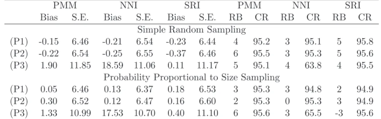
Table 1 presents the simulation results based on 2,000 Monte Carlo samples. When the covariate is 2-dimensional, all three imputation estimators have small biases, even when the mean function is misspecified. In addition, the proposed jackknife method provides valid coverage of confidence intervals for the predictive mean matching and stochastic regression imputation estimators in all scenarios. This suggests that the proposed replication method can be used widely even for stochastic regression imputation. When the covariate is 6-dimensional, nearest neighbor imputation presents large biases and low coverage rates.
6. Discussion
Propensity score matching has been recently proposed for inferring causal effects of treatments in the context of survey data; however, their asymptotic properties are underdeveloped (Lenis et al.; 2017). Because causal inference is inherently a missing data problem (e.g., Ding and Li; 2017), the proposed methodology here can be easily generalized to investigate the asymptotic properties of propensity score matching estimators with survey weights.
Table 1: Simulation results: Bias (×102) and S.E. (×102) of the point estimator, Relative Bias of jackknife variance estimates (×102) and Coverage Rate (%) of 95% confidence intervals.
PMM NNI SRI PMM NNI SRI
Bias S.E. Bias S.E. Bias S.E. RB CR RB CR RB CR Simple Random Sampling
(P1) -0.15 6.46 -0.21 6.54 -0.23 6.44 4 95.2 3 95.1 5 95.8 (P2) -0.22 6.54 -0.25 6.55 -0.37 6.46 6 95.5 3 95.3 5 95.6 (P3) 1.90 11.85 18.59 11.06 0.11 11.17 5 95.1 4 63.8 4 95.5
Probability Proportional to Size Sampling
(P1) 0.05 6.46 0.13 6.37 0.18 6.53 3 95.3 3 94.8 2 94.9 (P2) 0.30 6.52 0.12 6.47 0.16 6.60 2 95.3 0 95.3 3 94.9 (P3) 1.33 10.99 17.53 10.70 0.40 11.10 6 95.6 3 65.5 -3 95.6 PMM: predictive mean matching; NNI: nearest neighbor imputation; SRI: stochastic regression imputation.
Instead of choosing the nearest neighbor as a donor for missing items, we can consider fractional im-putation (Kim and Fuller; 2004; Yang and Kim; 2016) using K (K >1) nearest neighbors. Such extension remains an interesting topic for future research.
Appendix
A1 Proof for Theorem 1
Based on the decomposition in (6), writen1/2{µˆPMM(β∗)−µ}=DN(β∗) +BN(β∗), (A1)
whereDN(β) andBN(β) are defined in (7) and (8), respectively. For simplicity, we introduce the following
notation: mi=m(xi;β∗) and ei=yi−mi.
Under Assumption 2, for the predictive mean matching estimator, mi(1)−mi =Op(1). Together with
Assumption 3, we derive the order ofBN(β∗) as
BN(β∗) = n1/2 N X i∈A 1 πi (1−δi)(mi(1)−mi) =Op(n−1/2) =op(1).
Therefore, (A1) reduces to
n1/2{µˆPMM(β∗)−µ}=DN(β∗) +op(1).
Then, to study the asymptotic properties of n1/2{µˆPMM(β∗)−µ}, we only need to study the asymptotic
properties ofDN(β∗). We express DN(β∗) = n1/2 N " X i∈A 1 πi{ mi+δi(1 +kβ∗,i)ei} −µ #
= n 1/2 N N X i=1 Ii πi −1 mi+n 1/2 N N X i=1 Ii πi −1 δi(1 +kβ∗,i)ei +n 1/2 N N X i=1 (mi−µ) + n1/2 N N X i=1 δi(1 +kβ∗,i)ei = n 1/2 N N X i=1 Ii πi −1 mi+n 1/2 N N X i=1 Ii πi −1 δi(1 +kβ∗,i)ei+op(1), (A2)
givennN−1=o(1). We can verify that the covariance of the two terms in (A2) is zero. Thus, the asymptotic
variance ofDN(β∗) is var ( n1/2 N N X i=1 Ii πi − 1 mi ) + var ( n1/2 N N X i=1 Ii πi − 1 δi(1 +kβ∗,i)ei ) .
The first term, asn→ ∞, becomes
Vm = lim n→∞ n N2E ( varp X i∈A mi πi !) ,
and the second term, asn→ ∞, becomes
Ve= plim n N2 N X i=1 1−πi πi δi(1 +kβ∗,i)2var(ei |xi).
The remaining is to show that Ve = O(1). To do this, the key is to show that the moments of kβ∗,i are
bounded. Under Assumption 3, it is easy to verify that
ω˜kβ∗,i≤kβ∗,i≤ω¯˜kβ∗,i, (A3)
for some constantsω and ¯ω, where ˜kβ∗,i=
Pn
j=1(1−δj)dij is the number of uniti used as a match for the
nonrespondents. Under Assumption 2, ˜kβ∗,i =Op(1) and E(˜kβ∗,i) and E(˜kβ2∗,i) are uniformly bounded over
n(Abadie and Imbens; 2006, Lemma 3); therefore, together with (A3), we have kβ∗,i =Op(1) andE(kβ∗,i)
andE(k2
β∗,i) are uniformly bounded over n. Therefore, a simple algebra yieldsVe=O(1).
Combining all results, the asymptotic variance ofn1/2{µˆPMM(β∗)−µ}is Vm+Ve. By the central limit
theorem, the result in Theorem 1 follows.
A2 Le Cam’s third Lemma
Consider two sequences of probability measures (Q(N))∞
N=1 and (P(N))∞N=1. Assume that under P(N), a
statistic TN and the likelihood ratiosdQ(N)/dP(N) satisfy
TN log(dQ(N)/dP(N)) → N 0 −σ2/2 , τ2 c c σ2
in distribution, as N → ∞. Then, under Q(N),
TN → N(c, τ2)
in distribution, asN → ∞. See Le Cam and Yang (1990), Bickel et al. (1993) and van der Vaart (2000) for textbook discussions.
A3 Proof for Theorem 2
LetP be the distribution of (xi, yi, δi, Ii), for i= 1, . . . , N, induced by the marginal distribution of xi, the
conditional distribution of yi given xi, the conditional distribution of δi given (xi, yi), and the conditional
distribution of Ii given (xi, yi, δi). Consider P to be restricted by the moment condition through the
pre-dictive mean function (1) with the true parameter valueβ∗. We can treat the consistent estimator ˆβ as the
solution to the normalized estimating equation
SN(β) = n1/2 N N X i=1 Ii πi δig(xi;β){yi−m(xi;β)}= 0. (A4)
To discuss the asymptotic properties of ˆµPMM( ˆβ), we rely on Le Cam’s third lemma and consider an
auxiliary parametric modelPβ defined locally around β∗ with a density
exp n1/2(β−β∗)Tτ β∗Vs−1SN(β∗)−2−1n(β−β∗)TΛ−1(β−β∗) E exp n1/2(β−β∗)Tτ β∗Vs−1SN(β∗)−2−1n(β−β∗)TΛ−1(β−β∗) . (A5) Because under Pβ∗
, SN(β∗) → N(0, Vs) in distribution, the normalizing constant in the denominator
con-verges to 1 as n→ ∞. The Fisher information under the parametric model (A5) is nΛ−1. Therefore, ˆβ is
efficient under (A5).
We now consider sequences that are local to β∗, β
N = β∗+n−1/2h, indexed by N. In our context, we
have the population sizeN goes to infinity with sample sizen. Consider (xi, yi, δi, Ii), fori= 1, . . . , N,with
the local shiftPβN (Bickel et al.; 1993). We make the following regularity assumptions:
Assumption A5 (i) The superpopulation model is regular (Bickel et al.; 1993, pp 12–13); (ii) underPβN: SN(βN) → N(0, Vs) in distribution, as n → ∞; (iii) τβ is nonsingular around β∗, and n1/2( ˆβ −βN) =
τ−1
β∗SN(βN)+op(1); (iv) for all bounded continuous functionsh(x, y, δ, I), the conditional expectationEβN{h(x, y, δ, I)| x, δ= 1} converges in distribution to E{h(x, y, δ, I)|x, δ= 1}, where EβN is the expectation with respect to
PβN.
Under (A5), the likelihood ratio underPβN is log(dPβ∗/dPβN ) = −hT τβ∗V −1 s SN(β∗) +1 2h T Λ−1h+o p(1) = −hTτ β∗V −1 s SN(βN)− 1 2h TΛ−1h+o p(1),
where the second equality follows by the Taylor expansion ofSN(β∗) atβN.
We can derive that underPβN,
n1/2{µˆ PMM(βN)−µ(βN)} n1/2( ˆβ−βN) log(dPβ∗ /dPβN) → N 0 0 −1 2 hTΛ−1h , V1 γ1Tτβ−∗1 −γ1TVs−1τβ∗h τ−1 β∗γ1 Λ −h −hTτ β∗Vs−1γ1 −hT hTΛ−1h (A6)
in distribution, as n → ∞. Here, we write µ = µ(βN) to reflect its dependence on βN. We then express
µ(βN) =µ(β∗) +γ2T(n−1/2h) +o(n−1/2), and use the shorthandµforµ(β∗).
By Le Cam’s third lemma, underPβ∗
, we have n1/2{µˆ PMM(βN)−µ} n1/2( ˆβ−β N) → N −γT 1Vs−1τβ∗h−γ2Th −h , V 1 γ1Tτβ−∗1 τ−1 β∗ γ1 Λ
in distribution, as n→ ∞. Replacing βN byβ∗+n−1/2h yields that under Pβ
∗ , n1/2{µˆ PMM(β∗+n−1/2h)−µ} n1/2( ˆβ−β∗) → N −γT 1Vs−1τβ∗h−γ2Th 0 , V 1 γ1Tτβ−∗1 τ−1 β∗ γ1 Λ in distribution, as n→ ∞.
Heuristically, if the normal distribution was exact, then
n1/2{µˆPMM(β∗+n−1/2h)−µ} |n1/2( ˆβ−β∗) =h∼ N −γ2Th, V1−γ1TV
−1
s γ1. (A7)
Givenn1/2( ˆβ−β∗) =h, we have β∗+n−1/2h= ˆβ, and hence ˆµ
PMM(β∗+n−1/2h) = ˆµPMM( ˆβ). Integrating
(A7) over the asymptotic distribution of n1/2( ˆβ−β∗
), we derive n1/2{µˆPMM( ˆβ)−µ} ∼ N 0, V1−γ1TV −1 s γ1+γ2TΛγ2 . (A8)
The formal technique to derive (A8) can be find in Andreou and Werker (2012). (A8) gives the result in Theorem 2.
In the following, we provide the proof to (A6). Asymptotic normality of n1/2{µˆ
PMM(βN)−µ} under
PβN follows from Theorem 1. Asymptotic joint normality ofn1/2( ˆβ−β
N) and log(dPβ
∗
/dPβN) follows from
Assumption A5. Therefore, the remaining is to show that, underPβN:
DN(βN) SN(βN) → N 0 0 , V1 γ1T γ1 Vs (A9)
in distribution, asn → ∞. To prove (A9), consider the linear combination c1DN(βN) +cT2SN(βN), which
has the same limiting distribution as
CN = c1 n1/2 N N X i=1 Ii πi −1 m(xi;βN) +c1 n1/2 N N X i=1 Ii πi − 1 δi(1 +kβN,i){yi−m(xi;βN)} +cT 2 n1/2 N N X i=1 Ii πi −1 δig(xi;βN){yi−m(xi;βN)}, givennN−1 =o(1).
We analyze CN using the martingale theory. First, we rewriteCN =PNk=1ξN,k,where
ξN,k =c1 n1/2 N Ik πk −1 m(xk;βN) +c1n 1/2 N Ik πk −1 δk(1 +kβN,k){yk−m(xk;βN)} +cT 2 n1/2 N Ik πk − 1 δkg(xk;βN){yk−m(xk;βN)}.
Consider theσ-fieldsFN,k=σ{x1, . . . , xN, δ1, . . . , δN, y1, . . . , yk, I1, . . . , Ik}for 1≤k≤N. Then,{Pik=1ξN,k,FN,i,1≤
i ≤ N} is a martingale for each N ≥ 1. Therefore, the limiting distribution of CN can be studied using
the martingale central limit theorem (Theorem 35.12, Billingsley; 1995). Under Assumption 2, and the fact that kβN,k has uniformly bounded moments, it follows that
PN
k=1EβN(|ξN,k|
2+δ) → 0 for some δ > 0. It
then follows that Lindeberg’s condition in Billingsley’s theorem holds. As a result, we obtain that under
PβN, C
N → N(0, σ2) in distribution, as n → ∞, where σ2 = plimPNk=1EβN(ξ
2
N,k | FN,k−1). Assumption
A5 further implies the following expressions:
σ2 = plim N X k=1 EβN(ξ2N,k| FN,k−1) = c2 1plim n N2 N X k=1 EβN " I k πk −1 m(xk;βN) 2 | FN,k−1 # +c2 1plim n N2 N X k=1 EβN Ik πk −1 δk(1 +kβN,k){yk−m(xk;βN)} 2 | FN,k−1 ! +2cT 2plim n N2 N X k=1 EβN " Ik πk −1 2 δk(1 +kβN,k)g(xk;βN){yk−m(xk;βN)}2| FN,k−1 # c1 +cT 2plim n N2 N X k=1 EβN " Ik πk −1 2 δkg(xk;βN)g(xk;βN)T{yk−m(xk;βN)}2| FN,k−1 # c2
= c21plim n N2varp X k∈A mk πk ! +c21plim n N2 N X k=1 1−πk πk δk(1 +kβ∗,k)2σ2(xk) +2cT 2plim n N2 N X k=1 1−πk πk δk(1 +kβ∗,k)g(xk;β ∗ )σ2(xk)c1 +cT 2plim n N2 N X k=1 1−πk πk δkg(xk;β∗)g(xk;β∗)Tσ2(xk)c2 = c21Vm+c21Ve+ 2cT 2γ1c1+cT2Vsc2.
By the martingale central limit theorem, underPβN,(A9) follows.
A.4 Proof for Theorem 4
The replication method implicitly induces replication weightsω∗
i and random variablesuisuch thatE∗(ω∗iui) =
N−1π−1 i and var ∗ (ω∗ iui) =N−2(1−πi)π−i 2, fori= 1, . . . , N, whereE ∗ (·) and var∗
(·) denote the expectation and variance for the resampling given the observed data. For example, in delete-1 jackknife under probability proportional to size sampling withnN−1 =o(1), we haveω(k)
i = (n−1)
−1nω
i if i6=k, andω(kk)= 0. Then,
the induced random variables ui follows a two-point mass distribution as
ui= ( 1, with probability n−1 n , 0, with probability 1n, and weights ω∗ i = (n −1) −1nω
i. It is straightforward to verify that E∗(ω∗iui) = ωi = N−1π−i 1 and
var∗{(ω∗
iui)2}= (n−1)−1ωi2≈n−1N−2(1−πi)πi−2.
The kthe replication of ˆβ, ˆβ(k), can be viewed as one realization of ˆβ∗
which is the solution to the estimating equation S∗ N(β) =n1/2 X i∈A ω∗ iuiδig(xi;β){yi−m(xi;β)}= 0. (A10)
Let P∗ be the distribution ofz∗
i = (ωi∗uixi, ωi∗uiyi, ω∗iuiδi, ω∗iuiIi), for i= 1, . . . , N, given the observed
data induced by bootstrap resampling satisfying
E∗ {S∗ N( ˆβ)} = n1/2E ∗ " X i∈A ω∗ iuiδig(xi; ˆβ){yi−m(xi; ˆβ)} # = n 1/2 N X i∈A 1 πi δig(xi; ˆβ){yi−m(xi; ˆβ)}= 0,
and E∗n S∗ N( ˆβ)S ∗ N( ˆβ)T o = E∗hn S∗ N( ˆβ)−SN( ˆβ) o n S∗ N( ˆβ)−SN( ˆβ) oTi = nE∗ " X i∈A ω∗ iui− 1 N πi 2 δig(xi; ˆβ)g(xi; ˆβ)T{yi−m(xi; ˆβ)}2 # = n N2 X i∈A 1−πi π2 i δig(xi; ˆβ)g(xi; ˆβ)T{yi−m(xi; ˆβ)}2.
We consider an auxiliary parametric modelPβ defined locally around ˆβ with a density
expnn1/2(β−βˆ)Tτ β∗Vs−1SN∗( ˆβ)−2−1n(β−βˆ)TΛ−1(β−βˆ) o E∗hexpnn1/2(β−βˆ)Tτ β∗V −1 s SN∗ ( ˆβ)−2−1n(β−βˆ)TΛ−1(β−βˆ) oi. (A11)
Consider sequences that are local to ˆβ,β∗
N = ˆβ+n−1/2h, indexed by N, and zi∗, for i= 1, . . . , N, with
the local shiftPβ∗
N. We make the following regularity assumptions:
Assumption A6 (i) Model (A11) is regular; (ii) under Pβ∗
N: S∗ N(β ∗ N) → N(0, Vs) in distribution, as n → ∞; (iii) n1/2( ˆβ∗ −β∗ N) = τ −1 β∗S ∗
N(βN∗) +op(1); (iv) for all bounded continuous functions h(zi∗), the
conditional expectation E∗ β∗ N{h(z ∗ i)} converges in distribution to Eβ∗ˆ{h(z ∗ i)} , where Eβ∗ N is the expectation with respect toPβ∗ N.
Under (A11), the likelihood ratio underPβ∗
N is log(dPβˆ/dPβN∗) = −hTτ β∗Vs−1SN∗( ˆβ) + 1 2h Tτ β∗Vs−1τβ∗h+op(1) = −hTτ β∗V −1 s S ∗ N(β ∗ N)− 1 2h Tτ β∗V −1 s τβ∗h+op(1),
where the second equality follows by the Taylor expansion ofS∗
N( ˆβ) at β ∗ N.
The kthe replication of ˆµPMM( ˆβ), ˆµPMM(k) ( ˆβ(k)), can be viewed as one realization of
ˆ µ∗ PMM( ˆβ ∗ ) =X i∈A ω∗ iui[m(xi; ˆβ∗) +δi(1 +kβˆ∗,i){yi−m(xi; ˆβ ∗ )}]. (A12)
We can derive that underPβ∗
N, the sequence [ n1/2{µˆ∗ PMM(βN∗ )−µˆPMM(βN∗)} n1/2( ˆβ ∗− β∗ N)T log(dP ˆ β/dPβ∗ N)]T
has the same limiting distribution as in (A6). Then, following the same argument in the proof of Theorem 2, we can obtain that the asymptotic conditional variance ofn1/2µˆ∗
PMM( ˆβ
∗
), given the observed data, isV2.
The remaining is to show that, underPβ∗
N given the observed data:
n1/2{µˆ∗ PMM(βN∗)−µˆPMM(βN∗)} S∗ N(βN∗) → N 0 0 , V1 γ1T γ1 Vs (A13)
in distribution, as n → ∞. To prove (A13), given the observed data, consider the linear combination
c1n1/2{µˆ∗PMM(β∗N)−µˆPMM(βN∗)}+c2TS∗N(βN∗), which has the same limiting distribution as
C∗ N = c1n1/2 N X i=1 Ii ω∗ iui− 1 N πi m(xi;β∗N) +c1n1/2 N X i=1 Ii ω∗ iui− 1 N πi δi(1 +kβ∗ N,i){yi−m(xi;β ∗ N)} +cT 2n1/2 N X i=1 Ii ω∗ iui− 1 N πi δig(xi;βN∗){yi−m(xi;βN∗)}.
This is because underPβ∗
N, the extra term inC∗
N compared withc1n1/2{µˆ∗PMM(βN∗ )−µˆPMM(βN∗)}+cT2SN∗(βN∗) is n1/2 N X i=1 Ii N πi δig(xi;βN∗){yi−m(xi;βN∗ )} = n 1/2 N N X i=1 Ii πi δig(xi; ˆβ){yi−m(xi; ˆβ)}+Op(βN∗ −βˆ) = 0 +Op(n−1/2) =op(1). We analyze C∗
N using the martingale theory. First, we rewriteC ∗ N = PN k=1ξ ∗ N,k,where ξ∗ N,k = c1n1/2Ik ω∗ kuk− 1 N πi m(xk;βN∗) +c1n1/2Ik ω∗ kuk− 1 N πi δk(1 +kβ∗ N,k){yk−m(xk;β ∗ N)} +cT 2n1/2Ik ω∗ kuk− 1 N πi δkg(xk;βN∗){yk−m(xk;βN∗ )}.
for 1≤k≤N. Consider the σ-fields
F∗
N,k =σ{x1, . . . , xN, I1, . . . , IN, δ1, . . . , δN, y1, . . . , yN, ω∗1u1, . . . , ωk∗uk}
for 1≤k≤N. Then, {Pi
that underPβ∗ N, C∗ N → N(0,σ˜2) in distribution, as n→ ∞, where ˜ σ2 = plim N X k=1 E∗ β∗ N(ξ ∗2 N,k| FN,k−1) = c2 1plimn N X k=1 E∗ β∗ N " Ik ω∗ kuk− 1 N πi m(xk;βN∗) 2 | FN,k−1 # +c2 1plimn N X k=1 E∗ β∗ N Ik ω∗ kuk− 1 N πi δk(1 +kβ∗ N,k){yk−m(xk;β ∗ N)} 2 | FN,k−1 ! +2cT 2plimn N X k=1 E∗ β∗ N " Ik ω∗ kuk− 1 N πi 2 δk(1 +kβ∗ N,k)g(xk;β ∗ N){yk−m(xk;β∗N)}2c1| FN,k−1 # +cT 2plimn N X k=1 E∗ β∗ N " Ik ω∗ kuk− 1 N πi 2 δkg(xk;βN∗)g(xk;βN∗)T{yk−m(xk;βN∗)}2| FN,k−1 # c2 = c21plim n N2 N X k=1 Ik(1−πk) π2 k m(xk; ˆβ)2+c21plim n N2 N X k=1 Ik(1−πk) π2 k δk(1 +kβ,kˆ )2{yk−m(xk; ˆβ)}2 +2cT 2plim n N2 N X k=1 Ik(1−πk) π2 k δk(1 +kβ,kˆ )g(xk; ˆβ){yk−m(xk; ˆβ)}2c1 +cT 2plim n N2 N X k=1 Ik(1−πk) π2 k δkg(xk; ˆβ)g(xk; ˆβ)T{yk−m(xk; ˆβ)}2c2 = c2 1plim n N2 N X k=1 1−πk πk m(xk;β∗)2+c21plim n N2 N X k=1 1−πk πk δk(1 +kβ∗,k)2σ2(xk) +2cT 2plim n N2 N X k=1 1−πk πk δk(1 +kβ ∗,k)g(xk;β∗)σ2(xk)c1 +cT 2plim n N2 N X k=1 1−πk πk δkg(xk;β∗)g(xk;β∗)Tσ2(xk)c2.
Therefore, by the martingale central limit theorem, conditional on the observed data under Pβ∗
N, (A13)
follows.
References
Abadie, A. and Imbens, G. W. (2006). Large sample properties of matching estimators for average treatment effects, Econometrica 74: 235–267.
Abadie, A. and Imbens, G. W. (2008). On the failure of the bootstrap for matching estimators,Econometrica 76: 1537–1557.
Abadie, A. and Imbens, G. W. (2011). Bias-corrected matching estimators for average treatment effects,
Journal of Business & Economic Statistics 29: 1–11.
Abadie, A. and Imbens, G. W. (2016). Matching on the estimated propensity score,Econometrica84: 781– 807.
Andreou, E. and Werker, B. J. (2012). An alternative asymptotic analysis of residual-based statistics, Rev Econ Stat94: 88–99.
Berg, E., Kim, J. K. and Skinner, C. (2016). Imputation under informative sampling, J. Surv. Statist. Methodol. 4: 436–462.
Bickel, P. J., Klaassen, C., Ritov, Y. and Wellner, J. (1993). Efficient and Adaptive Inference in Semipara-metric Models, Johns Hopkins University Press, Baltimore.
Billingsley, P. (1995). Probability and Measure, 3 edn, Wiley: New York.
Chen, J. and Shao, J. (2000). Nearest neighbor imputation for survey data,J. Offic. Stat. 16: 113–131. Chen, J. and Shao, J. (2001). Jackknife variance estimation for nearest-neighbor imputation, J. Amer.
Statist. Assoc.96: 260–269.
Ding, P. and Li, F. (2017). Causal inference: A missing data perspective,arXiv preprint arXiv:1712.06170 . Fuller, W. A. (2009). Sampling Statistics, Wiley, Hoboken.
Kim, J. K. and Fuller, W. A. (2004). Fractional hot deck imputation,Biometrika 91: 559–578.
Kim, J. K., Fuller, W. A., Bell, W. R. et al. (2011). Variance estimation for nearest neighbor imputation for US Census long form data,The Annals of Applied Statistics 5: 824–842.
Kim, J. K., Navarro, A. and Fuller, W. A. (2006). Replication variance estimation for two-phase stratified sampling, J. Amer. Statist. Assoc.101: 312–320.
Le Cam, L. and Yang, G. L. (1990). Asymptotics in Statistics: Some Basic Concepts, Springer: Berlin. Lenis, D., Nguyen, T. Q., Dong, N. and Stuart, E. A. (2017). It’s all about balance: propensity score
matching in the context of complex survey data, Biostatisticsp. kxx063.
Little, R. J. (1988). Missing-data adjustments in large surveys,Journal of Business & Economic Statistics 6: 287–296.
Morris, T. P., White, I. R. and Royston, P. (2014). Tuning multiple imputation by predictive mean matching and local residual draws,BMC Med Res Methodol14: 75.
Otsu, T. and Rai, Y. (2016). Bootstrap inference of matching estimators for average treatment effects, J. Amer. Statist. Assoc. p. DOI:10.1080/01621459.2016.1231613.
Rubin, D. B. (1986). Statistical matching using file concatenation with adjusted weights and multiple imputations, Journal of Business & Economic Statistics4: 87–94.
Rust, K. F. and Rao, J. N. K. (1996). Variance estimation for complex surveys using replication techniques,
Stat Methods Med Res 5: 283–310.
Shao, J. and Steel, P. (1999). Variance estimation for survey data with composite imputation and nonneg-ligible sampling fractions, J. Amer. Statist. Assoc.94: 254–265.
van der Vaart, A. W. (2000). Asymptotic Statistics, Cambridge University Press, Cambridge, MA.
Vink, G., Frank, L. E., Pannekoek, J. and Buuren, S. (2014). Predictive mean matching imputation of semicontinuous variables,Statistica Neerlandica 68: 61–90.
Wolter, K. (2007). Introduction to Variance Estimation, 2 edn, Springer, New York.
Yang, S. and Kim, J. K. (2016). Fractional imputation in survey sampling: A comparative review, Statist. Sci.31: 415–432.