Nonspherical vapor bubble collapse

Thesis by

Richard Bruce Chapman

In Partial Fulfillment of the Requirement.s

For the Degree of Doctor of Philosophy

California Institute of Technology Pasadena, California

1970

ACKNOWLEDGMENTS

TABLE OF CONTENTS

Chapter Page

1. INTRODUC TION 1

A. Topics in Nonspherical Bubble Collapse I

B. Numerical Sirnula tion of Bubble Collapse 5

II. AN EXAMINATION OF THE PROBLEMS TO BE SOLVED

BY NUMERICAL SIMULATION 12

A. Definition of the Problems of Interest 12

B. General Characteristics of a Numerical Method Suited

to These Problems 17

III. DESCRIPTION OF THE NUMERICAL METHOD 20

IV.

V.

VI.

VII.

A. The Use of Finite Time Steps 20

B. The Finite Difference Equations 21

C. Solution of the Star Equations Using the Liebmann

Method with Overrelaxation 25

D. The Condition at Infinity Applied to the Outer Boundary 29 E. The Application of a Series of Nets to Obtain a Detailed

Solution 38

F. Calculation of Velocities on the Free Surface 45 G. Special Treatment for the Initial Time Step and the

Early Stage of Collapse 48

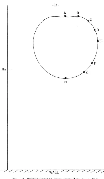
COLLAPSE NEAR A SOLID WALL A. Results of Numerical Simulation B. Discussion of Results

COLLAPSE OF INITIALLY NONSPHERICAL BUBBLES A. Results of Numerical Simulation

B. Discussion of Results

EVALUATION OF THE NUMERICAL METHOD A. Accuracy

B. Stability

C. Validity of Assumptions THE EFFEC T OF GRAVITY

54 54 66 71 71 77 79 79

89

91

94

APPENDIX

A. Garabedian's Estimate of the Relaxation Factor Applied

to Axially Symmetric Case 106

B. An Estimate of the Viscous Stresses on Nonspherical

Bubble 108

Abstract

Vapor bubble collapse problems lacking spherical sym-metry are solved using a method of simulation designed especial-ly for these problems. Viscosity and compressibility in the liquid are neglected. The method of simulation uses finite time steps and features an iterative technique for applying the boundary con-ditions at infinity directly to the liquid a finite distance from the free surface. Two cases of initially spherical bubbles collapsing near a plane solid wall were simulated, a bubble initially in con-tact with the wall and a bubble initially half its radius from the wall. at the closest point. In both cases the bubble developed a jet directed towards the wall. Free surface shapes and velocities are presented at various stages in the collapses. Velocities are scaled like

j ~p

where p is the density of the liquid and

~p

is the difference between the ambient liquid pressure and the vapor

~p 6 ( cm ) Z 1 atm. .

pressure. For - _p = 10 - - '" d .ty

f

t the Jet had a sec enSl 0 wa er

speed of about 130m/ sec in the first case and 170 m/ sec in the second when it struck the opposite side of the bubble. Collapse in a homogeneous liquid was simulated for bubbles with nonspherical initial shapes described by the

and rs = Ro[l - /0 Pz{cos8)] degree Legendre polynomial.

radi.i r s = Ro[l

+

/0 Pz{cos 8)] where P (cos 8) is the second

z

Bubble shapes in both cases were close to those predicted by linearized theory. A simple perturba-tion study oLthe effect of a small pressure gradient on a collapsing bubble shows that gravity is ordinarily negligible for bubbles

1. INTRODUCTION

A. Topic s in Nonspherical Bubble Collapse

The study of the behavior of a bubble in a liquid is greatIy simplified by the assurrlption of spherical symnlctry. Followin.g Rayleigh's[ 1) classical analysis of a problem first solved by

Be~;ant,

the inviscid collapse of a spherical cavity in a homogeneous, Incorn -pressible liquid under a constant ambient pressure, numerous Cluthor:,; have studied the behavior of spherical bubbles under a wide range of conditions. Far less is known about the nonspherical behavior (jf bubbles. Because problems lacking spherical symmetry have proven. too com,plex for direct analysis, they have been i.nvestigated primari-ly by qUiiljt~tive reasoning, experiments, and perturbations from spherically sym,metric solutions. One result of these studies has been the theory that cavitation damage is caused by the action of liquid jets forHled on bubbles near a solid surfac) 2).

resulting solution suggested a reentrant jet for a high degree of deformation. This jet formation was only speculative, howev~'r, sinc~e it is not unlikely under any circurnstance for a series of

Legendre fUllctions to display singular behavior near the axis of sym -Inc try when the series is considered outside its range of validity.

The irnportance of the influence of a solid boundary on bubble collapse as a possible factor in cavitation damage was further e mpha-sized by Plesset[ 4] who argued that the stresses caused by the col-lapse and subsequent rebound of a spherical bubble containing a small amount of permanent gas falls off rapidly as the distance from the bubble is increased. These stresses are too small to damage a solid boundary unless the boundary is quite close to the bubble. Thus a

sohel wall tHust have an irnportant effect on the collapse of any bubble capable of damaging it.

Experiments by Benjamin and Ellis[ 5] confirmed that jets form on bubbles collapsing near a solid wall. Large vapor bubbles, generally about one centimeter in radius, were grown from small nuclei by the application of a negative pressure. High speed photo-graphs were taken of these bubbles as they collapsed near a plane

solid surface. The ambient pres sure was maintained at about 0.04 atm eluring collapse so that collapse velocities would be reduced to facili-tate the photography. These bubbles were nearly spherical as they started collapsing. First they became elongated in the direction

10 meters/second. Benjamin and Ellis concluded that since velocitiu,<-;

are scaled like the square root of the pressure, the jet speed under

atmospheric am,bient pressure would be increased by a factor of about

five. It should be remarked, however, that the characteristic pressure

in this case is not the ambient pressure but the difference between the

ambient pressure and the vapor pressure inside the bubble. Because

the vapor pressure of water at room temperature is not negligible

cOlnpared to 0.04 atm., the scaling factor should be greater

than five. This problem will be explored more fully in Chapter IV.

Another m.ajor topic in nonspherical bubble studies has been

the behavior of small asymmetries of a nearly spherical bubble in an

infinite, homogeneous liquid. The distortion of the shape of a nearly

spherical bubble is commonly expanded in spherical harmonics so

that the radius of the bubble is

<Xl

r

s(8,rp,t) = R(t)

+

L

n=l

a (t) y

n n (I -1 )

where Y

n is a spherical harmonic of degree n. For perturbation

solutions the coefficients a (t) are assumed to be much _n smaller than

the mean radius R(t).

The central problelTI is the solution of a (t) for a given func-n

tion R(t) and a set of initial conditions. If the problelTI is linearized,

the various harlTIonics uncouple[ 6]. The general linearized equation

for a (t) was solved for bubbles collapsing or expanding under a n

constant ambient pressure by Plesset and Mitchell[ 7 ], who were able

One important result is that as the mean radius collapses to zero, 1

an(t) grows in magnitude like R -4: and oscillates with increasing

frequency. Thus even a small asymrnetry will become important

after the bubble has shrunk sufficiently.

Naude and Ellis[ 8] used the theory of Plesset and Mitchell to

analyze their experilnental study of the collapse of nearly hernispher-ical bubbles. Using electric sparks, they generated roughly

hemi-spberical bubbles on a plane solid surface and photographed them. as

they collapsed. Since the solid wall acts as a plane of symmetry, the

theory of Plesset and Mitchell is directly applicable.

A perfectly helnispherical bubble would, of course, remain

helnispherical as it collapsed and could be described by a spherically

symmetric theory such as Rayleigh's. The asymmetry in this case is

due to initial asymmetry in shape or velocity rather than the presence

of the soliel wall. Such bubbles can exhibit a wide range of behavior,

depending on the initial conditions, including the formation ( ) f a jet on

the axis of symlnetry. Although the solution of Plesset and Mitchell

does not require the lower harmonics to dominate as does Rattray's

solution for the collapse of an initially spherical bubble near a plane

wall, the assumption that i a

I «R means

that the linearized solution n

cannot be used to describe the jet formed on a nearly hemispherical

bubble at the ti=e that it strikes the wall.

The analysis by Naude and Ellis showed that the distortion in

the shape of their bubbles was prilnarily composed of the second ha

r-lnonic with a slnall contribution from the fourth harmonic. No odd

it (t) a (t)

l 4

Nauc16 and Ellis presented the eXperilTICntal vahws of

aroJ

and il((,)

l 4

over the first h;:df of the collapse (1.0 > R(t) > 0.5). These vahles agree with the perturbation solution. Since the contribution frorn the

second harrnonic was fairly large, Naude and Ellis had to add the

second order effect of a (t) on a (t) to obtain close agreement in the

Z 4

fourth harmonic. This second order effect was solved using an as -sumption analogous to Rattray's, that the lowest harmonic was

dorninant.

Because the photographic techniques used so effectively by

Benjarnin and Ellis had not yet been developed, it is not pos sible to

observe jetting directly from the photographs of Naude and Ellis.

They were able to produce some pitting in soft aluminum, however.

Similar experiments by Shutler and Mesler[

9J

also produced pitting. Shutler and Mesler concluded that jets formed but were too weak to

cause the pitting which they attributed to rebound bubbles. These

results were later challenged by Benjamin and Ellis.

B. Numerical Sirnulation of Bubble Collapse

The advantages of a numerical technique for simulating

non-spherical bubble collapse arc clear . Experiments are difficult and

give only sketchy results. Perturbations frorn sph('l'icaJly r;ymmetric

solutions are not valid for large deformations. A numerical sol.ution,

however, can check results and supply detailed information.

Numer-i.cal methods can also be applied to situations which might be very

difficult to produce in the laboratory.

technique to nonspherical bubble collapse have not yet been tiuccess-ful. A report by Mitchell, Kling, Cheesewright, and Hammitt[ 10J considers the feasibility of using the MAC method for this purpose. Before this report is discussed, the MAC method will be briefly described.

The Marker-and-Cell technique is a general method for

sim.ulating incornpres sible, viscid flows with an as sortment of bound-ary conditions including free surfaces. In practice it has been applied only to two-din1ensional problel11s, either plane or axially symmetric flows. The basic calculations are Eulerian. A domain in the two-din1ensional Eulerian space is covered by a grid of rectangular cells. The tJressure and the velocity are assumed to be nearly constant over a single cell. The pressure distribution is specified by its value at the center of each cell. The horizontal velocity u and the vertical velocity v are specified at the midpoints of the vertical and hori-zontal sides of each cell, respectively, as illustrated in Fig. 1.

The pressure and the two components of velocity are related through the continuity equation and the two components of the equation of lTlotion. These three equations can be combined to give an exprcs-sion for the Laplacian of the pressure as a function of the components of the velocity and their fir st and second space derivatives. In the

plane flow case, for example,

(I -2)

./

/'

V

u eP 4 U

v

Fig. 1 Cell Us,.d bV the MAC lvl<:thoc

I

t

/

,./

{

/

1

/

VAPOR

/

J

V

V

/

V

LIQUID

J'

V

/

V

F:ie(. Z Hcprcsent".tion 01 the P,ul>b10

, 11]

Welch, Harlow, Shannon and Dali .

The calculations progress by a series of finite time >oteps or

cycles. At the beginning of each cycle the velocity field is known so

that the right-hand side of Eq. (1-2) can be evaluated at each cell.

Poisson's equation can then be solved by some iterative technique.

Once the pressure distribution is known, it can be combined with the

known velocities in the equation of motion to find the derivatives of

both components of velocity with respect to time. These derivatives

are used to establish the velocity at each cell for the next cycle Lit

later. The final step in the cycle is to displace the nlarkers, which

represent sluall particles lUoving with the fluid. In practice there

will be several of these lUarkers in each cell. Their velocities are

found by sin1ple interpolation. These markers are used to represent

streamlines and to define the shape of the free surfaces. The manner in which a cell is treated during a cycle depends on whether it is a

full cell containing markers, an empty cell without markers, a free

surface cell containing markers but ac.jacent to an empty cell, or

sorne special case such as a cell adjacent to a solid boundary. After a certain an10unt of bookkeeping (detern1.ining which cells are full, etc.), the next cycle is ready to begin.

Mitchell, Kling, et al raised two n1ain questions in their report.

The first question, a comn1on one in flow sin1ulation, is how should

the calculations be initiated. They considered bubble collapse caused

by an instantaneous decrease of the pressure inside the bubble fron1

calculations was not justified; any discontinuity should be smoothed

out completely by the initial cycle of the MAC method. The point

remains, however, that the initiation of the calculation,; must: be ex

-cll11ined closely. It will be seen that an analysis of the early st'Lgc of

bubble collapse made in Chapter III of this thesis results in improved

accuracy and efficiency over this portion of the collapse.

The second question is how can a flow in an unbounded region

be described in a necessarily bounded domain. The collapse of a

ble is driven by the difference between the pressure inside the

bub-ble and the pressure infinitely far away. Although interest is

center-ed on the flow near the bubble, the far field cannot be ignored.

Rayleigh's solution for the collapse of a spherical bubble stated that

the difference between the pressure of the liquid and the ambient

pressure is the surn of two terms, which decrease in magnitude like

_1 _4

d and d as d, the distance from the bubble center, is increased.

For nonspherical collapse the pressure will have asymmetric terms, -2

which decrease like d and faster. One crude method of applying

the ambient pressure might be to extend the outer boundary of the

domain a number of radii away from the bubble and take the pressure

on the outer boundary to be the ambient pressure. A more refined

method was provided by Mitchell, Kling, et aI, who suggested that

Rayleigh's solution for the pressure be used at the outer boundary.

The outer boundary should be far enough away from the wall so that

the asymmetric terms will have died out. This method is based on

the linearized assumption that the spherically symmetric part of the

method presented in Chapter III of this thesis avoids this assumption

by using an iterative technique for applying the condition at infinity

directly to the outer boundary.

Another consideration in applying the .MAC rnethod to bul)bJ(,

collapse is one of stability. The theory of PIes set and Mitchell

shows that even a small error , or disturbance on the bubble surface, can become significant as the bubble collapses. Any finite difference

method will, of course, introduce small errors over the length of a

single cell. However, the MAC method is especially crude at free

surfaces and can easily give large errors that obscure the results. These errors arise because the MAC method does not modify the

finite difference equation at an irregular boundary such as a free

boundary but sin,ply imposes the condition that the pressure at the

center of a free surface cell is equal to the pressure on the free

sur-face. Modified finite difference equations at an irregular bounuary,

usually referred to as irregular stars, are essential for an accurate solution near the boundary. In their numerical study of

finite-an,plitude water waves Chan, Street, and Strelkoff[ 12] observed that

the waveforms beCalTIe unstable after a few cycles using the MAC

n,ethod. They obtained satisfactory results, however, with their

SUMMAC method, a modified MAC technique using irregular stars

at the free surface.

It is apparent that the problem of nonspherical bubble collapse

is one which is not readily solved by a general flow simulation method

principles. This is done most efficiently if the problems of greatest

II. AN EXAMINATION OF THE PROBLEMS TO BE SOLVED

BY NUMERICAL SIMULATION

A. Definition of the Problems of Interest

One problem of interest in nonspherical collapse is to

deter-mine the effect of a plane solid wall in deforming a collapsing bubble.

Typically a spherical bubble and the liquid surrounding it are visual

-ized as being at rest under a uniform ambient pressure until t '" 0

when the pressure inside the bubble is instantaneously reduced by

D.p. For a con~pressible liquid this instantaneous pressure drop will

produce a shock and an instantaneous radial velocity at the bubble

surface[ l3]

at t = 0+ (II -1 )

An alternate visualization of the problem, entirely equivalent

in the incompressible limit, is useful because it eliminates the

question of shocks and is more realistic experimentally. The bubble

is grown from a small nucleus by the application of a negative ambient

pressure. As the bubble grows the ambient pressur e is increased

continuously to the desired value where it is held constant. The

bub-ble will reach some maximum size and then collapse under the constant

ambient pressure. For spherically symmetric growth all segments of

the bubble surface will be at rest when the bubble reaches its maximum

size. In the incompressible limit the entire liquid will also be at rest.

With the absence of shocks compressibility will not become important

until speeds in the liquid are comparable with the speed of sound.

understanding that solutions are valid for small Mach nUlnbt,rs only.

The asymmetries caused by the solid wall should be separated

£I'orn those due to initial asymmetries in shape or velocity of the type

;:lllalyzed by Plesset and Mitchell. The bubble is therefore t<lkcn to be:

initially spherical and at rest,and any other extraneous asymm(;tric

effects such as gravity are also omitted.

The easiest and most widely applicable problem is one which

neglects all nonessential features. Therefore the following

assump-tions will be made.

1. The liquid is incompressible.

2 The flow is nonviscous.

3. The vapor pres sure is uniforITl throughout the bubble

interior.

4. The anlbicnt pressure and the vapor pressure arc constant

with tirne.

5. The bubble contains no permanent gas.

6. Surface tension effects are negligible.

Onlythefirstthreeassumptionsare essential to the method of

simulation developed in this thesis. The last three assumptions are

nlade to keep the essential features of the problem in the foreground.

For most cases of bubble collapse the viscous stresses are much

smaller than the inertial stresses. Thus in descriptions of bubble

collapse .. viscosity is usually neglected or kept only as n. "mall

refine-ment. Unlike the spherically symmetric case, which is always

ir-rotational, viscosity must be neglected in nonspherical collapse if

uniform pressure inside the bubble, this assumption will rernain valid

as long as speeds on the bubble surfa.ce are below the speed of sound

in the vapor.

The problem is specified by the Iollowing conditions:

p ::: an1bicnt pressure,

oJO

p ::: vapor pressure inside the bubble, v

R ::: initial radius of the bubble, o

b ::: initial distance from the plane wall to the

c enter of the bubble.

Because the flow is taken to be irrotational, the velocity

-vector v can be written in terms of a velocity potential rp

--

v(x, t) ::: Vrp(x,

-

t)

(II - 2 )

(II -3 )

(II -4)

(II -5)

(II -6 )

The liquid is assvmed to be incompressible so that rp must satisfy

Laplace's equation throughout the liquid,

2

-V rp(x, t) ::: 0 (II -7)

The pressure boundary conditions, (II-2) and (II-3), can be

restated in terms of

rp

and v:::

I

Vrpl

with the aid of Bernoulli's

equation

ocp

vZ

£.

at

+

"2

+

p ::: c(t) (II -8 )

Infinitely far from the bubble the velocity is zero, and the pressure is

the ambient pressure. The velocity potential is an arbitrary ft~ncli()n

of time only. Because this function of time has no physical

...

l~IT1it'l'(x, t) = 0 I ~ I-ex)

and since v - 0 at infinity,

Then on the

8'1'

at+

c (t) - p ex)

r

free surface,

vl Pex)-Pv

2 = p

(II -9)

~P

=

p (II-IO)

On the solid wall the cOIT1ponent of velocity norIT1al to the wall IT1ust be

zero. Thus

at the solid wall, (II-II)

8

where

ihi

denotes the derivative normal to the solid surface. The

condition that the liquid is initially at rest IY\ay be stated as

-'I' (x, t)

=

constant

=

0 when t __ 0 _(II-I2)

The generality of this probleIT1 becoIT1es evident when it is

stated in its nondiIT1ensional forIT1. Let the nondiIT1ensionalized

quantities be teIT1porarily denoted by a star. Then the nond

iIT1ension-alized velocity and displaceIT1ent are

-

--~ _v

-

_x

V;:~ and :x;:' _Ro (Il-13 )

JAP

_p

so that

t,:, =

~ojApP

'1',:, = 'I'

,

etc.

I¥

R

Laplace I S equation is unchanged in the nondimensional form as are

the homogeneous boundary conditions, (II-9) and (II-II), and the

homogeneous initial condition (II-12). The only changes are in the

initial conditions, (II-4) and (II-5), and the boundary condition (II-IO)

which have the nondimensional form:

R

o,:, co initial radius = 1

b,:, = initial distance frornwall to center of bubble

=-and

=

(II-I4)

-~

,(Il-l 5) R

o

(II-I6)

Thus the problem is completely characterized by the single

parameter

R

b The inclusion of surface tension or other effects o

would have added more parameters and reduced the general

applica-bility of the solution. Now that the nondimensionalized form has been

introduced, Eqs. (Il-I4), (II-I5), and (II-I6) will be used, but the star notation will be dropped in the sequel.

Another problem of interest is the collapse of a bubble with sOlne asynlmetry in its initial shape. A numerical solution is

extreme-ly difficult for any three dimensional problem not possessing at least

axial symmetry. The shape of any axially symmetric bubble can be described by its radius,

00

r s (8, t) - R(t)

+

I

n=I

a (t)P (cos 0)

n n (II -17)

where P is the n'th Legendre polynomial. The odd coefficients

vanish for cases with both pl<me and a.xial symmetry. These cases

are convenient because the same method developed for collapse near a

plane wall may be applied directly to problems with both plane and

:1.."ial syrrllTletry with the wall forming a plane of symmetry. If it were

desired, of course, this m.ethod could be easilymodifieu to eliminate

the wall.

The same assumptions can apply for this type of problerTl as

for the collapse near a solid wall. The nondimensional forms arc also

equivalent with the characteristic length being

R _o = R(O) = mean radius at t = 0

Instead of just a single parameter this problem is characterized

by an infinity of parameters:

a (0)

n

R o

and

a

(0)

n

n = 2 , 4 , 6 .

B. General Characteristics of a NUITlerical Method Suited to These Problems

Now that the problcITls of interest have been defined, the

general features of a method of flow simulation especially suited to

them can be discussed. Clearly the irrotationality of these problems

is best exploited by solving them in terms of the velocity potential.

A single variable gives a great simplification to almost every aspect

of the calculation. If desired, both the velocity and the pressure can

be easily calculated from a solution in terms of the potential.

interest in these probletns is centered on the flow at and near the i"r",' SlIrrdC('. '['hv shape' "f the coJ.lajJ"ing bubble is of Lll' gJ.'Cdt('1'

s'igllifi,'anu' tilan i' rklai.led d<:sc' L'iptlon of the stl'c;lInJiIH.!S [;11:

f,'(),,,

iii"

bubble, Markers like those used in the Marker-and-Cell method are of little use in representing the results. The task of defining the free surface can be perfortned by alternate methods so that marker s are not needed,

The method used in this thesis calculates the velocity only on

the bubble surface, The potential should vary most rapidly near the bubble and vary quite slowly far from the bubble, Thus it is neces-sary to have a highly accurate and detailed solution near the bubble surface, For a finite difference method this tneans that the grid should

be finest near the free surface, This can be accorrlplished either by a single nonuniforn1 grid or a series of grids with each successive grid more closely confined to the immediate neighborhood of the bubble and finer than the preceeding grid. The later method is the one used for

calculations in this thesis for reasons discussed in Chapter III. The

need for an accurate solution in the neighborhood of the free surface

also emphasizes the necessity of using irregular stars.

A basic question in the numerical simulation of axially

sym-n1ctric bubble collapse is whether to base the finite difference scheme on spherical coordinates as was suggested by Mitchell, Kling, et al

or on cylindrical coordinates. One advantage of spherical coordinates

is that a regular grid in spherical space with the origin inside the

bub-ble will have a greater concentration of points near the bubble than

the spherical system can present a problem, however, especially if

the bubble is highly deformed. Because of the singularity, the origin cannot be placed in or adjacent to the liquid. Another (litladvantag" oj"

spherical coorclinatctl is that the boundary condition at the wall cannot.

III. DESCRIPTION OF THE NUMERICAL METHOD

A. The Use of Finite Time Steps

All problems considered are axially symmetric so that the bub-ble and the liquid surrounding it can be described in any half plane bounded by the axis of symmetry. These problems are also assurrwd

to contain a plane solid wall or a plane of symmetry so that they can be further reduced to a single quadrant.

The method of flow simulation is based on a series of finite

time steps. The shape and the potential distribution of the free sur-face forming the bubble is known at the beginning of each time step.

The boundary condition at the free surface combined with the condition

at infinity and the boundary conditions at the solid wall and the axis of

syrnmetry will determine the potential throughout the liquid. The

velocities of points on the free surface can then be calculated. If the

time step At is small enough, the velocities will remain relatively

unchanged throughout the time step. Then the displacement of a point on the free surface with velocity v is approximately

-> -+

Ax = v A t (III -I )

Bernoulli's equation is used to get the rate of change of the potential of a point moving with the free surface,

acp

+ v z

~

(IIl-2)

where the nondirnensional variables have been used. F or L>t

slnall the change in the potential of a rlisplaced point on the free stlr

-i:lce is approximately

(IIl-3 )

The velocities in equations (III-I) and (IlI-3) are, of course, computed

at the beginning of the time step. After the free boundary has been

displaced and the potentials on it changed accordingly, the new bubble

shape with the new potential distribution on the free surface can be

used for another time step.

B. The Finite Difference Equations

The finite difference rnethod for solving the potential problem

is based on a cylindrical coordinate system (r, z). The r coordinate

measures the distance from the axis of symmetry, and the z

coordi-nate measures the distance from the solid wall or the plane of

sym-metry. Laplace's equation in the case of axial symmetry is

(III-4 )

Finite difference approximations to Laplace's equation can be

found in many places. Shawl 14], in particular, describes the

ap-proximation to Eq. (III-4). The domain of interest in the (1', z) plane

is covered with a square grid or net formed by a family of horizontal

z

2

3

o

4

r

Yi.'), . . ~ f\!llrnbf'rin~~ ~ystl,rn for Starn

AXIS OF SYMMETRY

vertical (r = constant) net lines parallel to tlw axis of Hytnnwtry.

Lines of both families are separated by a constant distance h called

the me sh length. The potential distribution thr oughou t the liquid is

described by the potentials of points, . called nodal points, where the

two families of net lines intersect. The free boundary is represented

in the calculation by the set of points where the free surface and the

net lines intersect (see Fig. 2).

A typical nodal point and its four neighboring nodal points,

each il distance h fron1 the central point, form a regular s';ar. If a

st:Jr is centered in the liquid but is ncar the free surface, sorne of its

outer nodal points may fall inside the bubble. Such stars are called

irregular stars because the nodal point inside the bubble must be

re-placed by a free surface point of known potential creating a leg

short-er than the meE;h length h. Stars centered inside the bubble are not

used in the calculations. The positions of points in both regular and

irregular stars with respect to the central or 0 point ar e identified

by the numbering system illustrated in Fig. 3.

The finite difference equation at a star is derived by ex

pand-ing the potential about the central point and neglecting the higher

derivatives (see Shaw, for example). The equation for most regular

stars is

cp

(

1

+

2

h

1

+

cP

(I

-

~)

+

cP

+

cP - 4cp =

0

1 r 3 tor 4 Z a

0 , 0

(III-5)

where cpo is the potential at the i'th point of the star and r is the

1 0

distance of the central point from the axis of symmetry. Equation

point in terms of the potentials of the other points of the star.

(III-G)

Both the boundary conditions on the solid wall and the boundary condi

-tions on the free surface require special treatment for certain star s.

Stars centered near the axis of symlTIetry also need special considera

-1

tion because of the r'l'r tCrlTI in the Laplacian. 'I' can be expanded

for constant z in powers of r about the axis of symmetry,

'I' = a

+

brl

+

.

(r small, z constant) (III-7 )

A linear terlTI cannot be present in the expansion of (0 as a

function of r with z fixed since it would imply a line source of fluid

on the axis. For a regular star centered on the axis of symmetry

1)

4

('I' -'I' 0)

lim ('I'

+ -

'I' = 4b'" _-.:...1 _ _

r -> 0 rr r r I}

(III-8 )

Thus the finite difference approximation is

'I'

+

'I'

+ 4'1' -

6'(1

= 0

2 4 1 a (III -9)

or

'1'0 (III -10)

Stars centered directly adjacent to the axis of symmetry at

r = h should also be considered. The equation for these stars is also

derived from an expansion about the axis of symmetry for constant z.

(III -1 1 ) Since the solid wall forms a plane of symrnetry, star s centered on the wall must satisfy

(III -12)

This condition is imposed simply by using the appropriate star equa-tion with <p substituted for <p •

Z 4

The boundary condition at the free surface enters the calcula-tion through the irregular stars. Equacalcula-tions for these stars contain the sizes of the irregular legs as parameters but are derived in the same way as the corresponding regular star equations. One very minor exception is a star centered at r = h with an irregular point 3

(the point closest to the axis of symmetry). The potential cannot De expanded about the axis in this case because there is no liquid at the axis. The irregular version of Eq. (III- 6) is used for this rare

case.

C. Solution of the Star Equations Using the Liebmann Method with Overrelaxation.

Each star equation can be written as a formula for the potential of the central point of the star in tenns of the central potentials of neighboring stars. The Liebmann iterative method is used with over-relaxation to find the potential distribution that solves all star equa-tions simultaneously. Each iteration of the Liebmann method covers every star in the net column by column. The central potential at each

This procedure is in contrast with another comnlOn method, the Richardson method, which does not use the new potentials until an iteration has been cornpleted. An initial estimate of the potential distribution is necessary to start the Liebmann method. Usually this is provided by the potential distribution from the preceeding time step. The first tim.c steps and time steps immediately following a change in the nets are initiated from a uniformly zero potential.

The convergence of the Liebmann method for large nets is greatly accelerated by the use of overrelaxation[ 15]. Suppose _{'P s} is the potential of the central point that satisfies the star equation. Then the old potential cP old is replaced by

cP new = cP old

+

a(cp s - cP old)

1 :;; a

<

2 (III -13 )

The constant a is called the relaxation factor . A simple estimate of the optimum relaxation factor and the rate of convergence for large nets was developed for the plane case by P. R.

Garabedia~

16]. He estirnated that after N iterations the error would be reduced by a factor of the order of magnitude

E =o(e -qNh) _{(III -14)}

where q is defined by

(III -15)

0'

=

and k is the lowest eigenvalue of the problem

1

(III -16)

(III-I7)

The boundary conditions on U are the same as on the "rror in the

potential; U is zero on boundaries of known potential and has a 2cru

normal derivative on boundaries where the normal derivative is known.

An analysis analogous to Garabedian's is made of the axially

symmetric case in Appendix A. The results are identical if the

Laplacian in Eq. (IIl-17) is taken in its three dimensional form.

Clearly convergence is most rapid when q is maximized. Garabedian

pointed out that if C is made greater than

k/./2,

1 the real part of

- J4CZ - 2k2 will decrease sharply r educing convergence considerably,

1

but if C is less than or equal to the optimum

- j4C

2

- 2k2 is purely imaginary so that

1

2 (2 -0')

q= ~

k/.[2,

1 then

(III -18)

If we assume that 0' is large enough to cover the lowest eigenvalue,

i. e.

2

0'

?:.

---"k-hr--I

+

_1_

.f2

= 0' .

optlmum (III -19)

then the rate of convergence is a function of 0' only,

(III-20)

potential distributions on their surfaces. Let d measure thl' (iistancl!

from their common center. If the radii of the inner sphere and the outer sphere are d.

1 and d o respectively, the boundary condition on U is

U = 0 at d = d.

1 and d = d o (1II-21)

The eigenfunction with the smallest eigenvalue is a linear

cOlnbination of the zeroth order spherical Bessel functions,

a.nd y (k,r). FrOlTl the boundary conditions

o

where

sin k (d-d.)

1 1

U

-1 d

TI

k = d -d.

1 0 1

TI

= Jh

j (k, 1')

o

(III-22)

(1II-23)

is the smallest eigenvalue and J is the number of mesh lengths

be-tween spheres. The optimum relaxation factor is then

a . 2

optlmum =

-1

+

_iT _ _

i2J

(III-24)

If the relaxation factor is this optimum value, then the error reduction

factor is

(III - 25)

The number of iterations necessary to achieve a given error reduction

is proportional to J.

Liebmann method, and overrelaxation are all well-known techniques

that have been applied to many different problems. The more

special-ized aspects of the method associated with the present problem will

now be discussed.

D. The Condition at Infinity Applied to the Outer Boundary

It was stated in Chapter I that an iterative method has been

developed for applying the condition at infinity to the outer boundary.

The outer boundary in this case refers to the boundary of the net

exclud-ing the free boundary, the axis of symmetry, and the solid wall. The

method is based on a spherical coordinate system (d, e) with its origin

at the intersection of the axis of symmetry and the solid wall. The

distance from the origin is d; the angle with the axis of symmetry is

e.

Each step begins with a net like the one in Fig. 4. The shape of

this net is chosen to give the nodal points on the outer boundary a near

-Iy constant value of d. A slight point to point variation in d is

lln-ilnportant, however. Irregular stars are unnecessary on the outer

boundary. The average value of d on the outer boundary will be

referred to as d .

o

The potential can be expanded in a series of axially symmetric

harmonics that will be valid for values of d large enough to complete

-ly contain the bubble

00

<p (d e) = ' \ (A d Zk + B d-(Zk+ I)) P

,

L

z

k zk zk (cos e) • (III-26)

k=o

Only the even Legendre polynomials are used in the expansion because

'Lpproaches zero infinitely far from the bubble may be restat.ed as

A = 0

2 n n=1,Z,3. (TTl-27)

The A coefficients will be zero only when the potential distribution on

the outer boundary is consistent with the condition at infinity.

The higher harmonics should die out most rapidly as d incr

eas-es. It is assumed that d is large enough so that the P (cos e) and

o 0

P (cos e) terms effectively describe the potential on the outer boundary.

2

The P (cos e) term is also included in the calculation~but d is

4 0

large enough in practice to keep this term negligible. The potential at

the outer boundary may then be written as

+

B

2)

d 3

o

P

(cOSe)+(A

d 4

+

B4 )p(coso)

l 4 0 d S 4

o

=

c

+

c

P (cos e)

+

c

P (cos e)

o l 2 4 4 (IIl-Z8)

Each time step begins with a trial potential distribution on the

outer boundary. This potential distribution is usually provided by the

results of the previous time step. The potential problem is solved

using these trial outer boundary values for the potential. The condition

that the A coefficients must vanish may be stated as a relationship

be-tween the potential and its radial derivative. Therefore, the radial

derivative is calculated at each nodal point on the outer boundary. All

nodal points on the outer boundary of nets like the one in Fig. 4 have

other nodal points directly below them and to their left. The derivative

in the vertical direction can be calculated by fitting a second order

nodal points directly b(~low it. From Eq. (III-46)jwhich is derived HI Section F of this chapter, one obtains

o<p

haz

(r,z)

=

2(",(r, z) - '" (r, z-h) ) -

"2 ('"

1 (r, z) - <p (r, z - 2h) ) .(III-29)

The horizontal del"iv'ative is calculated by the same method and is then combined with the vertical derivative to produce the radial derivative:

B o

d l o

+(

2A d - 3 l 0

BZ)

P (cos 0) d 4 l

o

+

(4A d

3_

4 0 5 _d B4 6 )P(COSO) 4

o

_ D

+

D P (cos e)

+

D P (cos 0 )

o 2 2 4 4 (III-30)

The C and D coefficients are easily evaluated fr01TI the potential on the outer boundary and its radial derivative. The A and B coefficients are determined by the C and D coefficients. In pa rti cula r ,

B = - D d2

o 0 0

B = (2C d 3 _ D d 4) / 5

2 Z 0 2 0

and B = (4C d 5 _ D d 6 ) / 9

4 4 0 4 0 (III- 31)

C

=

B /d == - D d

o 0 0 0 0

C =B /d 3= (2C -D d )/5

z z 0 Z Z 0

C = B /d 5= (4C - D d )/9

4 4 0 4 4 0 (III-32)

With the neglect of the higher harmonics, Eqs. (III-32) will be satisfied

only when the potentials on the outer boundary are consistent with the

condition at infinity. Equations (III-32) suggest that the B coefficients

calculated fl-om Eqs. (III-3l) may be used to form new potentials at the

outer boundary nodal points from the formula

<p (d, 8)

B o = -d

+

B

z

d 3

B

P (cos 8) + -1 P (cos 8)

Z d 5 4

(III- 33)

The iteration scheme is to solve the potential problem with the

new outer boundary potentials, then find the B coefficients from Eqs.

(III-3l) and use them inEq. (III-33) to establish outer boundary pote

n-tials for the next iteration. Let a superscript n on a coefficient

denote the value of that coefficient during the n'th iteration. Equation

(lII-33) specifies that

C n+! _{= B n/ d - - Dnd}

0 o 0 0 0

n+1

Bn/d 3 (2Cn _Dnd )/5

C = =

Z Z 0 Z Z 0

n+ !

Bn/d 5= (4C' - rfd )/9 (III - 34)

C =

4 4 0 4 4 0

If the coefficients converge, they will converge to a solution of Eqs.

(III-32).

the simple case of a perfectly hemispherical bubble on a solid wall with an axially symmetric potential distribution on the bubble surface.

Let d. be the radius of the bubble. The potential on the bubble

sur-1

face ITlay be expanded as

()()

<p(el_i , 0) ::

L

FzkF

z k(cOS e)

k::o

Then the correct potential at the outer boundary is

(lI[-35)

3 5

<p (do,e)::

Fo(:~)

+ F

z(

:~)

_{P z} (cos e) + F4(

:~)

P₄(cos e) +. (IlI- 36)

The ratio

d.

1

d

is assumed to be sufficiently small so that higher o

harmonics are negligible at the outer boundary. Let the error in the potential at the outer boundary be expanded in Legendre polynomials:

(IIl- 37)

Then from Eq. (III-36) the coefficients are given by

( d. ) B n d.

En = C n F _1

=An+~-F1-1)

0 0 o d 0 d o d

0 0 0

F z(

:~)

3

B n

F z(

:~)

3

En _C n :: And Z + Z

::

- -

-Z Z Z 0 _{d 3}

0

F

4(

:~)

5 _Bn

(:~

)

5

En _{= C} n ₌ And 4+

- -

4

-

_F (IlI-38)

4 4 4 0 _d

5 4

0

Since the potential is known on the free surface the solution there is

n

+

B /d. =0 F

o 1 0

(III-39)

and

Equations (III-38) can be combined with Eqs. (III-39) to obtain

d d.

Bn = F d. + En~

o 0 1 0 d -d.

o 1

(III-40)

and

From Eqs. (III - 34) the C and E coefficients for the next iteration will be

C n+l

=

_{F (d}i

)+ En d.

(

E~+l

d.

1

=

En 1

0 o d 0 d -d.

,

0 d -d.

0 0 1 0 1

(d.

f

d:

,(

E~+l

d3

)

C n+l _{-. F} _1_

+

En 1

=

_En 1 _{, (III-41 )}

2 2 d 2 _{dl. -d~} 2 _d3 _-d~

0

0 1 0 1

and

(d. S ciS _{( n+l} ciS

)

C n +1 1 n 1

=

En 1

4

=

F ₄

d)

₀ + E ₄ , E

dS -d~ 4 4 _{d S -d~}

0 1 0 1

If d./d

a single iteration. It is now obvious why more terms were nol

includ-ed in the calculation to improve the validity for smaller values of d ;

o

convergence is enhanced by keeping the radius of the outer boundary

large. In practice three or four iterations were sufficient to establish

a satisfactory potential distribution on the outer boundary starting

from a uniformly zero distribution, and only a single iteration was

necessary to adjust for the small changes between consecutive time

steps.

The net used to establish the outer boundary potentials had a

radius of 40 m esh lengths or, occasionally, 50 mesh lengths. The

initial bubble shape had a radius of 5 mesh lengths in this net for thr.,

problem of an initially spherical bubble collapsing near a solid wall

and a mean radius of 10 mesh lengths for the problem of an initially

nonspherical bubble collapsing in a homogeneous liquid.

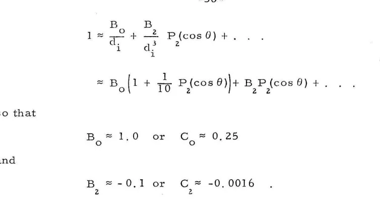
One case, for example, started with a nonspherical bubble

with a radius of

(III-42)

where

luean radius

=

1

=

10 mesh lengths

The radius of the outer boundary was four time s the mean

radius of the bubble. The potential was unity over the entire bubble

surface. Since the deviation from spherical (or hemispherical) was

only ten percent, a fir st order estimate of C and C can be made

o 2

B B

'"

;:r:-

0

+

_d] 2 P(cosO) _Z

+

1

1

(IIl-43 )

so that

and

B '" - O. I or C '" -0.0016

2 l

This gives a rough check on the values actually computed, which are

Iii'tecl ill Table 1. Differences are due to second order terms nc'glectcd

in Eq. (III-43) and the fact that the accuracy of the numerical solution

is lin.ited because the free surface is represented by only a finite

llurnber of points in this net, twenty-one in this case.

TABLE I

Values of the C Coefficients Computed while Establishing a Potential Distribution on the Outer Boundary

Cn C n Cn

0 2 4

Iteration

initial values 0.0 0.0 0.0

n = 1 0.28664 -0.0042862 0.0018235

0.24474 -0.00010602 -0.00057663

n 3 0.25159 -0.0014508 0.000044342

0.25038 -0.0013336 -0.000018905

n = 5 0.25060 -0.0013661 -0. 0000094077

An examination of Table I shows that the convergence of the co

-efficients does not follow Eqs. (III-41). The Cn coefficient converges

[image:40.525.74.451.60.266.2]

rnore rapidly than expected; while which should converge faster

Cn is sornewhat settled. n

than C ,

o does not converge at all until o Finally Cn,

4

which should converge the fastest of all, merely cic,cJ.ines

in magnitude without approaching a limiting value. One pos sible e

x-planation is that the asymmetry of the bubble shape has coupled the

co-efficients. If d. is no longer a constant, then Eqs. (III-39) will be

1

coupled causing the coefficients of the error to couple. But this

coup-ling cannot explain, for example, why C nand C n are erratic during

z

4

the first few iterations while C~ converges. The true cause is

reveal-ed by the observation that an increase in the number of iterations usreveal-ed

by the Liebrnann rnethoci reduces this type of behavior. Any change in

Cn or any other of the coefficients alters the outer boundary potentials o

and introduces an error in the potential solution near the outer boundary.

The Liebmann method reduces this error by a factor depending on the

number of iterations used. The overall effect of the reduced error

should be much smaller than the change in the potentials. But if the

changes in the outer boundary potentials are much larger than C or

z

C, the reduced error may still have a large effect on them. In this

4

case C

z

and C 11. 4

is much smaller than Co' and C is negligible.

4 Thus C n z

are highly susceptible to changes in Cn as has been observed. o

This does not pose a practical problem, however, since it is of no value

to determine C

z and C4 more accurately than Co.

The accuracy of the coefficients is enhanced by keeping the number of points used to repre sent the free surface as large as

pos-sible. Convergence demands that the outer boundary of the net be as

sirnultaneously satisfied for cases in which the bubble is close to the

solid wall. Then as the bubble collapses, the scale of the net used to

establish the outer boundary potentials can be halved from time to

time. This procedure effectively moves the outer boundary closer to

the free surface. The outer potentials are then re -established. In

practice these potentials were observed to be consistent with their

values during the preceeding time step when the new outer boundary

points were interior points. Values of the C coefficients for tirne

steps irnmedlately before and after a typical scale change are pre

-sented in Table II.

TABLE II

Values of the C Coefficients for Time Steps

Immediately Before and After a Typical Scale Change

C

2 C 4

time step preceeding scale change 0.1377 0.0002603 0.0000754

time step following scale change 0.2699 0.002600 -0.0000292

Ideally, neglecting the change between consecutive time steps, C

a

should be doubled and C increased by a factor of eight. The second

z

set of coefficients is the rnore accurate since the net used to find them

contained twenty-four free boundary points while the net used for the

fir st set contained only twelve free surface points.

E The Application of a Series of Nets to Obtain a Detailed Solution

Once the potentials on the outer boundary are established, they

l<!ngth of the net used to establish the outer boundary potentials giv(,s

only a rough solution nC'ar the free boundary. Therefor" a s<!ri.<!s of

progressively finer net;; is used to provide a l'l'lore detailed descrjption

there. A.J.1.other possibility would be to use a large sing.le net cornposed

of various regions of uniform mesh length with the mesh lengths of

these regions decreasing as the free surface is approached. This would

have one advantage in that a more detailed de'scription of the free sur-face would increase the accuracy of the outer boundary potentials. If

this single net contained a large number of points, however, the con

-vergenC'e of the Liebmann method could be quite slow. It can be seen

£1'on1 Garabedian's results that the number of Liebmann iterations

needed for a given factor of error reduction is, assuming a uniform

Hlesh, inversely proportional to the mesh length. Thus the total num

-bel' of operations required is inversely proportional to the cube of the n1.esh length. If a detailed solution of a potential problem is required, it is more economical to first obtain a solution using a coarse net and

. [ 17] h . f h

then apply the flner nets . T us a serles 0 nets is t e most

ef-ficient l'nethod for obtaining a detailed solution near the free boundary.

It is convenient if each net of the series has a mesh length half

the mesh length of the preceeding net. Then a nodal point of the finer

net falls either directly on the location of a nodal point in the precee d-ing net, midway between two such points, or equidistant from four of

NE

T

2

NET

Fig. 5 A Ty!)ical Series of Nets

The shapes of all nets except the first one of the series are arbitrary.

Usually these nets were shaped to give a minimum distance of ten to

twenty mesh lengths between the free surface and the outer boundary.

A typical series of nets is illustrated in Fig. 5.

In practice either three or four nets were used in the series.

The finer nets had a large percentage of their nodal points located in

the bubble interior. Although these "interior" points have no active

role in the calculations, they do occupy storag2. Sir-ce the number of

these points quadruples when the mesh length is halved, storage r equirc:

-ments can limit the number of nets that can be used in a series. For

an initially spherical bubble collapsing near a solid wall the final net

contained an average of 100 free surface points. Because of the plane

of symmetry, the final net contained an average of 50 free surface

points for the case of a nonspherical bubble with axial and plane

sym-metry collapsing in a homogeneous liquid. Whenever the number of

free boundary points fell below these levels, another net was added to

the series. Whenever the scale of the first net was halved, a net was

subtracted from the series.

The relaxation factor for the first net of the series was estirna

-ted from the model of a sphere of radius d with a point of known

o

potential (representing the free boundary) at its center. The optimum

relaxation factor for J = 40 is a = 1.895 from Eq. (III-24). After

N Liebmann iterations, the error will then be reduced by a factor of

E = O(exp(O. III N)). Thus 40 iterations will reduce the error by a

factor of about 85. This is enough to adjust for the small changes be

potentials between consecutive tiIne steps are always Inuch smaller than the change s at the free boundary. The potential probleIn is solved at least twice using the first net of each tiIne step, once to establish the new outer potentials and once using theIn. Thus the first net is subject to at least 80 iterations under the proper free bounda.ry condi-tions. If the outer potentials Inust be established froIn a uniforInly zero distribution, an increased nUInber of iterations such as 50 is advisable because of the large changes at the outer boundary.

The finer nets contain errors of predoIninantly SInal! wave-lengths. For these nets a relaxation factor capable of handling errors extending a distance of 20 Ineshlengths froIn a spherical boundary should be adequate. FraIn Eq. (III-24) a = 1.80 when J = 20. The initial errors in the finer nets will be sInall in Inagnitude. Also erJ:ors near the free boundary left by one net will be reduced by following nets. Therefore 15 iterations should be sufficient for the interm.edlate nets. This gives an error reduction factor of about 30 for a = 1.80. Al-though the initial errors are quite sInal!, Inore iterations are advisable for the final net of the series because the velocities at the free surface points are calculated £rOIn its solution. A choice of 25 iterations gives an error reduction factor of about 250 for a = 1.80.

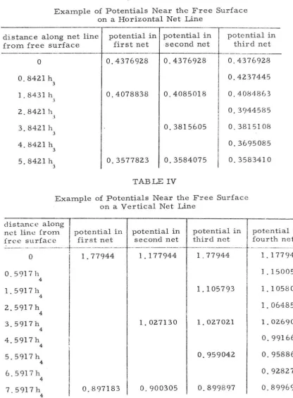
The potentials of typical points near the free surface as they appear in the various nets of the series give SOIne insight into the

The symbol h. refers to the mesh length of th,~ i't], net of the series.

1

TABLE III

Example of Potentials Near the Free Surface

on a Horizontal Net Line

distance along net line potential in potential in potential in

from free surface first net second net third net

0 0.4376928 0.4376928 0.4376928

0.8421h 0.4237445

3

1 . 8431 h 0.4078838 0.4085018 0.40~4863

3

2.8421h 0. 3<)44585

.\

3.8421 h 0.3815605 0.3815108

3

4.8421 h 0.3695085

3

5.8421 h 0.3577823 0.3584075 0.3583410

3

TABLE IV

Example of Potentials Near the Free Surface

on a Vertical Net Line

distance along

net line frorn potential in potential in potential in potential in

free surface first net second net third net fourth net

-

'

-

.

-

--

-

.. -

-

-

+

----.

-

- - -

-

+-

-

--1-- - - -_. -.--- -.-.----

-o

I

1.77944 1.177944 1.77944 1.177944

0.5917h 1.150050

4 1.5917h 4 2.5917h 4 3.5917h 4

4.5917h

4

5.5917h

4

6.5917h 4

7.5917h

4

1.027130

0.897183 0.900305

1.105793 1.105800 1.064858 1.027021 1.026908

0. 991664

0.959042 0.958863

0.928276

[image:47.529.66.483.122.688.2]

8

V

A/

0

V

/

D

7

E

.~l'.t.g. ;1 Puints Used to Calculate the VeJocif:;/ ;11: FrC'(; T)oUlldal")' - ... F-'r,int 1\

l~ig. 7

[] ORIGINAL POINTS A DISPLACED POINTS

o

NEW POINTS

Lne a 1" III te 1":)o.ia ti on to Obt ain

These eX-3.IT1ples show that the potential at a point changes only

slightly between consecutive nets of the series; the errors in the initial

potentials of the finer nets are sIT1all, as expected. They also show

that the potential in the final net varies SITlOothly with the distance from

the free boundary and can be described accurately by a quadratic over

the distance of a few IT1esh lengths. This behavior is useful in. the

velocity calculati.ons.

F. Calculation of Velocities on the Free Surface

The velocity components in both the r a n d z directions must

be found at all free boundary points of the final net. Each free houndary

point will lie on either a vertical net line or a horizontal net line. The

v{~locity calculation will be described for a point on a vertical. net line.

The ITlethod is cOIT1pletely analogous for points on horizontal net lines.

If the ITlesh length of the final net is sufficiently sITlall, each free

bound-ary point will be part of an irregular star with a regular point opposite

the free boundary point as in Fig. 6. The only exception for free

bound-ary points on vertical net lines occurs when the bubble touches the wall

with an acute angle of contact. Then there are stars with irregular

vertical legs centered on the solid wall. Let 'fB' 'Po' and <PD be the

potentials of the free boundary point, the central point of the irregular

star, and the point opposite the free boundary point, respectively. The

potential along the vertical net line is approxiluated near the free

boundary point by a quadratic fitted through points B, 0, and D.

'vVriting this quadratic as an expansion about the boundary point for a

(III-44)

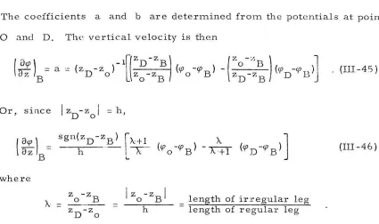
The coefficients a and b are determined from the potentials at points

o

::lnd D. The vertical velocity is then

Or, since

where

A: =

I

z -z

I

= h D o '

- -- - = z -z

D

0

= length of irregular leg

length of regular leg

.

(III-45)

(III-46)

When A. is smaller tl,an sorne minimum value A. M- , point D is used

In

in plac e of point 0, and the next point along the net line (point E in

Fig. 6)replacef; point D. This adds unity to A..

If the irregular star is centered on the solid wall, the potential

may be expanded about the wall along a vertical net line. Since the

potential is an even function of z,

'P = 'P _o

+

bz2

+

.

(for r = constant). (III-47)

Thus the verticill velocity may be approximatE:d by

8rp '" 2b z '"

8z

B

(III-48 )

Once the derivative in the vertical direction has been found, the

[image:50.525.66.491.114.366.2]

[re',' Goundary !Joints 011 either side oJ point 13, points A awl. C, l\

.linear approxirnation is used for the potential between adjacent fr"e

surface points. Expansion of the potential about point B along the

free surface gives to first order the form

(III-49)

Equation (III -49) produce s an estimate for the horizontal velocity,

'PA-'P B -

(~~)

(zA- zj3) B

(

~'P.

or

) . '" 13

(III-50)

To avoid any systernatic errors, this estimate is averaged with

another estinlate of

( o<{')

made using the free surface point C on

or

B

the other side of B, Since the method for finding the horizontal

veloc-ity is essentially to subtract the known vertical component from the

velocity tangential to the free surface, the tangent to the free surface

cannot be nearly vertical if accurate results are desired, If the

nor-rnal to the free t;urface makes too small an angle with the horizontal

dlrcction, then the velocities are not calculated at that point, and the

poill!: will lJot be llsed in forming the displaced [ree bOllDda.l'y [or th(~

ncx.t tirne step, Similarly free boundary points on horizontal net. Jines

arc 110t used where the normal to the free surface is nearly vertical,

The percentage of points eliminated by this criterion is small,

how-ever, since the free surface will cross few vertical net lines where its