RoseMerry: A Baseline Message level Sentiment Classification System

RoseMerry: A Baseline Message-level Sentiment Classification System

Huizhi Liang, Richard Fothergill and Timothy Baldwin

The University of Melbourne VIC 3010, Melbourne

[email protected], [email protected], [email protected]

Abstract

In this paper, we propose a baseline message-level sentiment classification method, as de-veloped for SemEval-2015 Task 10, Subtask B. This system leverages both hand-crafted features and message-level embedding fea-tures, and uses an SVM classifier for message-level sentiment classification. In pre-training the embedding features, we use one million randomly-selected tweets. We present re-sults over SemEval-2015 Task 10, Subtask B, as well as the Stanford Sentiment Treebank. Our experiments show the effectiveness of our method over both datasets.

1 Introduction

The rise of social media such as blogs and micro-blogs (e.g., Twitter) has fueled interest in sentiment analysis (Liu, 2012; Pang and Lee, 2008). One of the most popular settings for carrying out sen-timent analysis is at the sentence level or over in-dividual micro-blog posts, using the simple three-label class set of POSITIVE, NEGATIVE and NEU -TRAL(Liu, 2012; Pang and Lee, 2008; Rosenthal et al., 2014). Sentiment classification has been shown to have utility in various business intelligence ap-plications, including product marketing, identifying new business opportunities, and managing a com-pany’s reputation (Liu, 2012; Pang and Lee, 2008).

Learning effective features plays an impor-tant role in building sentiment classification sys-tems (Liu, 2012; Pang and Lee, 2008). For ex-ample, the winning system in the SemEval-2013 message polarity classification task (Nakov et al.,

2013) was based on a rich set of hand-tuned features such as word-sentiment association lexicon features, word n-grams, punctuation, and emoticons, which were combined using a simple SVM-based classi-fier (Mohammad et al., 2013). Recently, there has been a surge of interest in representation learning — automatically learning word and document rep-resentations, often in the form of continuous-valued vectors or “embeddings” — using auto-encoders or neural network language models (Mikolov et al., 2013; Le and Mikolov, 2014). Of particular rel-evance to message-level sentiment analysis, Tang et al. (2014) proposed a deep learning approach to learn sentiment-specific word representation fea-tures, and Le and Mikolov (2014) proposed a neu-ral network auto-encoder to learn message-level vec-tors.

In this paper, we detail RoseMerry, a (strong) baseline sentiment analysis method that combines hand-crafted features with message-level1 embed-dings generated by doc2vec (Le and Mikolov, 2014), using a linear-kernel SVM.

2 The Proposed Method

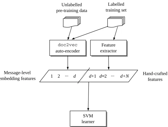
The proposed method combines a set of hand-crafted features with automatically-generated message-level representation features. The fea-tures are concatenated into a combined feature representation, and fed into a linear-kernel SVM learner usingLibSVM(Chang and Lin, 2011). The 1_{Throughout the paper, we will use “message” as a generic}

term to refer to both tweets and also sentences in the case of the Stanford Sentiment Treebank. Note that the method could potentially be applied to any granularity of document.

Labelled training set Unlabelled

pre-training data

Feature extractor

doc2vec

auto-encoder

Message-level embedding features

Hand-crafted features

SVM learner

d

2

1 ... d₊₁ d₊₂... ... d+N

Figure 1: System architecture

architecture of the method is shown in Figure 1.

Our interest in sentiment analysis stems from a desire to use it as part of a commercial text analyt-ics system. As such, there is an overarching con-straint associated with the system and all third-party components must be licensed in a manner which is compatible with commercial use. In our description below, we point out places where we were unable to use notable resources because of this constraint.

The message-level embeddings are pre-trained using doc2vecover the combination of the train-ing data and a random sample of 1M English tweets, as detailed in Section 2.1. The hand-crafted features are based heavily off the work of Mohammad et al. (2013), and are detailed in Section 2.2. Finally, the

d-dimensional message-level embedding is concate-nated with theN-dimensional hand-crafted features to form ad+N-dimensional combined feature vec-tor. We experiment with each of the two feature sub-sets, in addition to the combined feature set.

One significant divergence from Mohammad et al. (2013) is that we do not use many of the sentiment lexicons, due to non-commercial licensing. Given that one of the key findings in that work was that lex-icons are one of the most reliable features, we expect that this will have a large impact on our results.

2.1 Message-level embeddings

The message-level embeddings are generated us-ing doc2vec (Le and Mikolov, 2014). In this framework, words and documents are represented in a common d-dimensional space, using real-valued vectors. The embeddings are learned by prediction of each word in a given document based on the doc-ument embedding and word embeddings of its sur-rounding context. The document vector acts as an-other word which captures the larger context of a word that is missing from its immediate word con-text.

The word and document vectors are trained using stochastic gradient descent, based on back propaga-tion.

After pre-training, the document vector of each training document is used as its representation, and test documents are fed through the pre-trained auto-encoder to generate a message-level embedding.

2.2 Hand-crafted features

The hand-crafted features are largely lexical:

with one non-final word removed)

• charactern-grams: continuous features captur-ing the proportion of contiguous character n -grams (n∈ {3,4,5}) of each type observed in the training data, which make up a given mes-sage

• proportion of words in all caps: the proportion of words which are in all caps (e.g.YAY)

• punctuation features: the proportion of tokens which are made up of multiple exclamation marks, question marks, or a combination of the two (e.g.??!)

• elongated words: the proportion of words which have “elongated” vowels, i.e. a given vowel repeated more than twice (e.g.coool)

• proportion of emoticons: the proportion of to-kens which are (a) positive- and (b) negative-polarity emoticons, as identified by Chris Potts’ scripts2

• polarity of message-final emoticon: if the last token is a polarised emoticon, its polarity (NEGATIVE,POSITIVEor None)

• negated words: the presence or absence of words in “negated contexts”, where a negated context is defined as span from a negation word3_{to a punctuation mark (matching the} reg-ular expression[,.:;!?])

3 Experiments

In this section, we will detail the experimental setup and the results of our experiments.

3.1 Datasets

We evaluate our method over two labelled datasets, and also two unlabelled datasets to pre-train doc2vec, as detailed below.

2_{http://sentiment.christopherpotts.net/} tokenizing.html

3_{Defined based on Chris Potts’ word list: http://} sentiment.christopherpotts.net/lingstruc. html.

Training Development Test

Set Set Set

POSITIVE 3043 438 1038

NEGATIVE 1177 212 365

NEUTRAL 4082 542 987

Table 1: The number ofPOSITIVE,NEGATIVE,NEUTRAL

documents in the SemEval-2015 dataset

Training Set Test Set

POSITIVE 3606 444

NEGATIVE 3304 428

NEUTRAL 1623 226

Table 2: The number of POSITIVE, NEGATIVE and NEUTRALsentences in the Stanford Sentiment Treebank

dataset

3.1.1 Labelled Datasets

SemEval-2015 Dataset: the official

SemEval-2015 Task 10, subtask B dataset, comprised of tweets which have been hand-labelled for sentiment at the message-level (in terms ofPOSITIVE, NEGA -TIVE andNEUTRAL sentiment). The dataset is par-titioned into three components, as detailed in Ta-ble 1:4 _{(1) training set, (2) development set, and (3)} test set.

Stanford Sentiment Treebank Dataset: a

col-lection of movie review documents from www. rottentomatoes.com, which have been sen-tence tokenised and annotated for sentiment at the sentence level (Maas et al., 2011) and pre-partitioned into training and test data, as detailed in Table 2. Socher et al. (2013) additionally annotated the data at the phrase and lexical levels, but we use only the sentence-level annotations in this paper.

3.1.2 Unlabelled Datasets

Twitter Dataset: a random sample of 10M

En-glish tweets from a 5.3TB Twitter dataset crawled from 18 June to 4 Dec, 2014 using the Twitter Trend-ing API. This is used as additional data to pre-train the message-level embeddings for the SemEval-2015 Dataset.

IMDB Dataset: a 100K sentence movie review

dataset from www.imdb.com, collected by Maas 4_{As the labels have not been released for the progress test}

et al. (2011). This is used as additional data to pre-train the message-level embeddings for the Stanford Sentiment Treebank dataset.

3.2 Experimental setup

To evaluate the effectiveness of the different feature sets, we report on results as follows:

• RM-manual: only hand-crafted features

• RM-doc2vec: only message-level

embed-dings

• RM-all: both hand-crafted features and message-level embeddings

As our primary evaluation metric, we use F1PN, which is the average F1PN for the POSITIVE (i.e., F1pos) andNEGATIVEclasses (i.e., F1neg):

F1PN = F1pos+₂F1neg

We also report the overall classification accuracy (Acc) across the three classes, and the F1PN score of each class (i.e., F1pos, F1negand F1neu).

For the message-level embeddings, we usedd= 100 and a context window size of 10. We used LibSVMwith a linear-kernel and default parameter settings.

3.3 Experimental results

In this section, we present the results first over the SemEval-2015 datasets, and then over the Stanford Sentiment Treebank.

3.3.1 Results for SemEval-2015

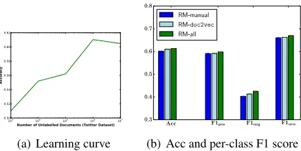
The results for the SemEval-2015 test set and progress test set are shown in Table 3. Figure 2a is a learning curve of RM-doc2vec, pre-trained over varying numbers of documents. We can see that the results plateau at 1M tweets; this is the document collection size we used for pre-training

RM-doc2vecandRM-allin our official runs. The overall Acc and F1 of each class for the three fea-ture sets are shown in Figure 2b. RM-doc2vecis marginally better thanRM-manualoverall, and for theNEGATIVE class in particular. When combined, RM-alloutperforms the two component feature sets across all classes, pointing to (weak) complementar-ity between the two feature sets.

103 104 105 106 107 Number of Unlabelled Documents (Twitter Dataset)

0.50 0.52 0.54 0.56 0.58 0.60 0.62

Ac

cu

ra

cy

(a) Learning curve

Acc F1pos F1neg F1neu

0.3 0.4 0.5 0.6 0.7 0.8

RM-manual

RM-doc2vec

RM-all

(b) Acc and per-class F1 score

Figure 2: The learning curve forRM-doc2vec, and the Acc, F1pos, F1neg, and F1neuresults for SemEval-2015

104 105 Number of Unlabelled Documents (IMDB Dataset)

0.58 0.59 0.60 0.61 0.62 0.63 0.64 0.65

Ac

cu

ra

cy

(a) Learning curve

Acc F1pos F1neg F1neu

0.0 0.2 0.4 0.6 0.8

1.0 RM-manual

RM-doc2vec

RM-all

(b) Acc and per-class F1 score

Figure 3: The learning curve forRM-doc2vec, and the Acc, F1pos, F1neg, and F1neuresults for the Stanford

Sen-timent Treebank

3.3.2 Results for the Stanford Sentiment Treebank

The learning curve for RM-doc2vec over the Stanford Sentiment Treebank with varying numbers of unlabelled (IMDB) documents is given in Fig-ure 3a. RM-doc2vec performed best when pre-trained over 50K documents (plus the Stanford Sen-timent Treebank data), and this is the model we include in the remainder of our results over this dataset. Figure 3b shows the Acc, in addition to the per-class F1 over the Stanford Sentiment Tree-bank for the three feature sets. The overall trend is strikingly similar to that for SemEval-2015, with the combined feature set performing marginally better than the two component feature sets in all cases.

4 Conclusion

pre-Test Set Progress Test Set

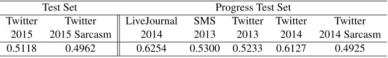
Twitter Twitter LiveJournal SMS Twitter Twitter Twitter 2015 2015 Sarcasm 2014 2013 2013 2014 2014 Sarcasm 0.5118 0.4962 0.6254 0.5300 0.5233 0.6127 0.4925

Table 3: The official evaluation results for the SemEval-2015 Test and Progress Test set (F1PN)

sented results over the SemEval-2015 dataset and Stanford Sentiment Treebank, and showed that the combined feature achieved the best results. The dif-ference between the combined feature set and the two component feature sets is not statistically signif-icant (based on randomised estimation, p > 0.05). While we were not able to achieve state-of-the-art results, we commend the proposed approach as a strong baseline method.

Acknowledgements

This research was supported by the Australian Re-search Council. The authors would like to acknowl-edge the support of Pitchwise (www.pitchwi. se), and also the coding assistance of Fei Liu.

References

Chih-Chung Chang and Chih-Jen Lin. 2011. LIBSVM: A library for support vector machines. ACM Transac-tions on Intelligent Systems and Technology, 2:27:1– 27:27.

Quoc V. Le and Tomas Mikolov. 2014. Distributed representations of sentences and documents. CoRR, abs/1405.4053.

Bing Liu. 2012. Sentiment Analysis and Opinion Min-ing. Synthesis Lectures on Human Language Tech-nologies. Morgan & Claypool Publishers.

Andrew L. Maas, Raymond E. Daly, Peter T. Pham, Dan Huang, Andrew Y. Ng, and Christopher Potts. 2011. Learning word vectors for sentiment analysis. In Pro-ceedings of the 49th Annual Meeting of the Associa-tion for ComputaAssocia-tional Linguistics: Human Language Technologies, pages 142–150, USA.

Tomas Mikolov, Kai Chen, Greg Corrado, and Jeffrey Dean. 2013. Efficient estimation of word represen-tations in vector space.CoRR, abs/1301.3781. Saif M. Mohammad, Svetlana Kiritchenko, and

Xiao-dan Zhu. 2013. NRC-Canada: Building the state-of-the-art in sentiment analysis of tweets. CoRR, abs/1308.6242.

Preslav Nakov, Sara Rosenthal, Zornitsa Kozareva, Veselin Stoyanov, Alan Ritter, and Theresa Wilson.

2013. Semeval-2013 task 2: Sentiment analysis in Twitter. In Second Joint Conference on Lexical and Computational Semantics (*SEM), Volume 2: Pro-ceedings of the Seventh International Workshop on Se-mantic Evaluation (SemEval 2013), pages 312–320, USA.

Bo Pang and Lillian Lee. 2008. Opinion mining and sentiment analysis. Foundations and Trends in Infor-mation Retrieval, 2(12):1–135.

Sara Rosenthal, Alan Ritter, Preslav Nakov, and Veselin Stoyanov. 2014. Semeval-2014 task 9: Sentiment analysis in Twitter. InProceedings of the 8th Inter-national Workshop on Semantic Evaluation (SemEval 2014), pages 73–80, Ireland.

Richard Socher, Alex Perelygin, Jean Wu, Jason Chuang, Christopher D. Manning, Andrew Y. Ng, and Christo-pher Potts. 2013. Recursive deep models for semantic compositionality over a sentiment treebank. In Pro-ceedings of the 2013 Conference on Empirical Meth-ods in Natural Language Processing, pages 1631– 1642, USA.