Environment and Growth

Munich Personal RePEc Archive

Environment and Growth

Horii, Ryo and Ikefuji, Masako

Tohoku University, University of Southern Denmark

February 2014

Online at

https://mpra.ub.uni-muenchen.de/53624/

Environment and Growth

∗

Ryo Horii, Tohoku University

Masako Ikefuji, University of Southern Denmark

February 2014

Abstract

This paper examines the implications of the mutual causality between

environmen-tal quality and economic growth. While economic growth deteriorates the environment

through increasing amounts of pollution, the deteriorated environment in turn limits

the possibility of further economic growth. In a less developed country, this link, which

we call “limits to growth,” emerges as the “poverty-environment trap,” which explains

the persistent international inequality both in terms of income and environment. This

link also threatens the sustainability of the world’s economic growth, particularly when

the emission of greenhouse gases raises the risk of natural disasters. Stronger

environ-mental policies are required to overcome this link. While there is a trade-off between

the environment and growth in the short run, we show that an appropriate policy can

improve both in the long run.

Keywords: Environmental Kuznets Curve, Limits to Growth, Poverty-Environment

Trap, Sustainability, Natural Disasters

∗_{The authors are grateful to Iain Fraser and Katsuyuki Shibayama for their helpful comments and} sugges-tions. We also thank Stefan Jungblut, Nobuyuki Hanaki, and the staffs at Paderborn University, GREQAM (Aix-Marseille University), and Kent University for the opportunity to write this paper. This study was financially supported by the JSPS Grant-in-Aid for Scientific Research (23730182, 23530394), DAAD, the Daiwa Anglo-Japanese Foundation, the Nomura Foundation, and the Asahi Breweries Foundation. All remaining errors are our own.

†_{Corresponding Author: Graduate School of Economics and Management, Tohoku University. 27-1} Kawauchi, Aoba-ku, Sendai 980-8576, Japan.

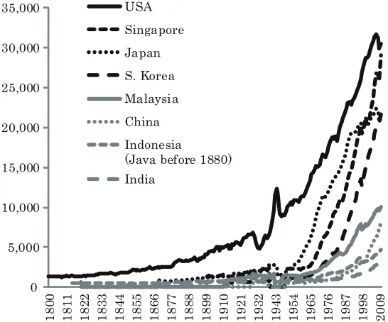
0 5,000 10,000 15,000 20,000 25,000 30,000 35,000 1 8 00 1 8 11 1 8 22 1 8 33 1 8 44 1 8 55 1 8 66 1 8 77 1 8 88 1 8 99 1 9 10 1 9 21 1 9 32 1 9 43 1 9 54 1 9 65 1 9 76 1 9 87 1 9 98 2 0 09 USA Singapore Japan S. Korea Malaysia China Indonesia (Java before 1880) India

Figure 1: Long-term evolution of per capita GDP in the U.S. and Asian countries (in 1990

international dollars).

1

Introduction

One of the most important and challenging questions for economists has been how to

harmonize economic growth with the natural world. Since the industrial revolution,

the growth rate of income per capita has been fairly stable in the United States. As

shown in Figure 1, the measured per capita real GDP in the U.S. has been expanding

exponentially, with its growth rate after the mid-19th century being around 2%. Figure

1 also shows that a number of Asian countries are in the process of catching up to the

U.S. income level. Although they differ in the timing when modern economic growth

took off (e.g., Japan’s modern growth started relatively earlier, while China’s rapid

growth is a much more recent phenomenon), their growth rates were typically higher

than the U.S. after the second half of the 20th century. As long as this trend

contin-ues, the per capita income of successful countries will converge to the exponentially

expanding U.S. per capita GDP level.

However, given that the world’s economic growth means the exponential expansion

of output, especially if it requires ever increasing inputs of natural resources, it is

obvious that this process cannot be continued for a very long time. This was the

theme investigated by Meadowset al. (1972) under the title of the ”Limits to Growth,”

which subsequently led to a large body of literature that examined the possibility of

1974; Smith, 1974; Stiglitz, 1974; see also a survey by Krautkraemer, 1998).

In addition to resource scarcity, the pollution that accompanies the production or

use of particular kinds of inputs poses another constraint for economic growth.

Al-though the literature on pollution and growth has largely been disjointed from that

on the resource scarcity,1_{the fundamental root of the problem is the same: the}

finite-ness of the natural environment. Suppose that the aggregate production function has

constant returns to scale and that all inputs are reproducible or non-exhaustible. In

such a setting, long-term growth is typically achieved by a homothetic expansion of all

inputs and outputs.2 _{However, if the production or use of some types of inputs involves}

pollution, such an expansion will result in an increasingly deteriorating environment.

Given that nature itself cannot be expanded along with other inputs, the intensity of

pollution (i.e., the ratio of pollution to environmental capacity) will increase with the

growing production. The deteriorated environment in turn makes sustained economic

growth difficult for a number of reasons, such as health problems and frequent natural

disasters caused by global warming. In the paper “Are there limits to growth?”, Stokey

(1998) considered this type of problem using an AK growth model with pollution and

showed that it is not optimal to pursue sustained growth as long as the technology

level is constant.

In this paper, we explain the implications of the interrelation between the

envi-ronment and economic growth. In particular, we focus on two issues. The first is the

feasibility of economic development in stagnant poor countries that are suffering both

from both low income and environmental degradation. Second, at the global scale we

consider the sustainability of world economic growth in the future. While these two

issues have so far been treated in two separate bodies of literature, we show that the

key to understanding both issues is the same: the mutual causality between the

envi-1

Theoretical models of economic growth that examine the relationship between pollution and growth often assumed away the finiteness of pollution-generating inputs. Besides the analytical tractability, one substantial reason for this is that when the emission of pollutants binds the possibility of economic growth, the constraint of resource scarcity becomes slack and will not affect the equilibrium or optimal outcome. Similarly, those that focus on the resource scarcity typically assume away pollution, because if the resource constraint is stricter, pollution will only have secondary effects on the possibility of economic growth. Nonetheless, some recent studies numerically examine the intricate interaction of pollution and the finiteness of resources and obtained quantitative implications of the interaction (for example, see Acemoglu et al. 2012).

2

pol

lut

ion (e

nvi

ronm

ent

al

de

gra

da

ti

on)

income (output)

・

Y=0 (limits to growth)

.

b (Environmental

Kuznets Curve)

P

Y

a

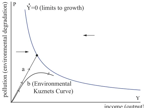
Figure 2: The relationship between income and pollution.

ronment and economic growth. After intuitively explaining how this interaction works

in the next section, we introduce two formal models that focus on the two issues in

sections 3 and 4.

2

Mutual causality between the environment and

economic growth

As we discussed in the introduction, we will inevitably face the “limits to growth”

problem if the environment continues degrading as the economy develops. The

con-sequences of “limits to growth” are illustrated in Figure 2, which depicts the mutual

relationship between pollution and the income level in one phase diagram. In the

fig-ure, the ˙Y = 0 curve reflects the causality from pollution to long-term income: for a

given intensity of pollutionPt, the output can grow up to the ˙Y = 0 curve in the long

run.3 _{The downward slope of this curve means that the potential for economic growth}

is adversely affected by environmental degradation. For example, when air pollution

harms human health (WHO, 2006), it not only lowers the productivity of workers but

also reduces life expectancy and, hence, the return on education, which in turn lowers

the incentives for parents to provide their children with higher education. Without

sufficient educated workers, (foreign) firms with advanced technologies will be

reluc-3

tant to invest in such regions. These considerations imply that higher pollution (i.e.,

environmental degradation) will adversely affect the long-term income.

What, then, determines environmental quality? We may think of economic growth

as a determinant of pollution. At the initial stage of economic growth, the scale of

production is small, and thus, both income and pollution would be small. In the

figure, this means that the economy starts from a point near the origin. Then, as the

economy develops, the scale of production increases. As long as the economy operates

under the same technology and the same relative factor prices, the pollution P would

increase proportionally with output. In the figure, this means that the economy moves

to the upper right direction and will eventually reach the ˙Y = 0 curve, beyond which

the economy cannot grow (denoted by path a).

While this seems a pessimistic result, in reality the technology level is not constant

but improves as income grows. If improved technologies cause less pollution for a given

amount of production, economic growth could mitigate the environmental problem

through technological change.4 _{This consideration leads to theEnvironmental Kuznets}

Curve (EKC), a hypothesis that there should be an inverted U-shaped relationship

between per capita income and various pollutants or environmental indicators. If

this hypothesis is correct, environmental degradation continues until the income per

capita reaches a certain level, but beyond it environmental quality will improve as

the economy grows. In Figure 2, the path denoted as b shows the movement of the

economy following this hypothetical EKC. If pollution begins to decrease before the

economy hits the ˙Y = 0 locus, it might be possible that the economy can grow beyond

the “limits to growth.” In fact, many studies, including seminal studies by Grossman

and Krueger (1991, 1995) and Selden and Song (1995), confirm the existence of the

EKC for local air pollutants, including sulfur dioxide (SO2), suspended particulate

4_{More precisely, there are both supply-side and demand-side factors behind the effect of economic growth}

Poverty-Environment trap

・

Y=0 (limits to growth)

.

sustained economic growth

・

pol

lut

ion (e

nvi

ronm

ent

al

de

gra

da

ti

on)

income (output)

P

Y better steady state

c

d

e

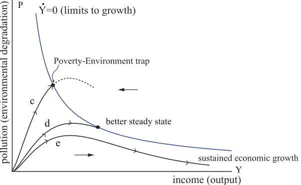
Figure 3: Poverty Environment Trap

matter (SPM), and oxides of nitrogen (NOx).

Note, however, that the existence of the EKC does not always mean that every

economy can overcome the “limits to growth.” Because of the differences in the

char-acteristics of countries, including technology, resource endowments and institutions

(particularly institutions for environmental protection), the shape and location of the

EKC vary across countries. Three paths in Figure 3 illustrate the consequences of

different EKC shapes. Pathcillustrates the case in which the economy hits the ˙Y = 0

curve before reaching the top of the EKC. At this point, the economy is trapped by

the mutual causality between environmental degradation and poverty. The

environ-mental quality is low because the economy is poor. Such an economy cannot afford

to employ better and cleaner technology because everyday consumption is their first

priority and they cannot finance the costs of required investments that would improve

their life and environment in the future. Similarly, it would be difficult for people in

such an economy to agree to set stricter environmental regulations because such

regu-lations would seem to (at least temporarily) further reduce their low incomes. At the

same time, the economy is poor because environmental degradation lowers the

pro-ductivity of workers, reduces their life expectancy, gives less incentives for parents to

provide good education for their children, and so forth. We call such a situation the

“poverty-environment trap”.

In Figure 3, pathdshows that an economy that maintains low pollution intensity

along the process of economic development can get over the top of the EKC and

Bangladesh China India

Japan Malaysia

Myanmar Nepal

Republic of Korea

Thailand

0 50 100 150 200 250

0 10000 20000 30000 40000 50000

a

n

n

u

a

l

m

ea

n

P

M

1

0

(u

g

/m

3

)

income per capita (current US$)

Figure 4: Income and Air Pollution in Asian countries.

concentrations in the capital city, where PM10 means particulate matter with a diameter of 10 µm or

less. Source: Urban outdoor air pollution database, Department of Public Health and Environment, World

Health Organization, September 2011. Per capita income is from World Development Indicators (WDI),

Worldbank.

those of economies trapped by the poverty-environment trap. Path e shows that it

is theoretically possible that an economy can grow indefinitely without facing limits

to growth. These considerations suggest that in the long run we will observe large

differences across countries in terms of the intensity of pollution and income level and

will also find a negative relationship between these two variables. Figure 4 confirms this

expectation, which shows that there is a negative relationship between air pollution

(PM10 concentrations) and the per capita income level among Asian countries. In

Section 3, we present a formal model with a microeconomic foundation that explains

the existence of multiple steady states—–the poverty-environment trap and a better

steady state—–and we discuss how the environment is related to international income

differences.

Pollution is a serious problem not only at the level of individual countries but also

at the global scale, particularly regarding the issue of global warming. In this case,

we should view the whole global economy as one entity because the emission of global

warming gases depends on the economic activities in all countries. Can we then observe

an inverted-U relationship between the average income in the world and the emission

0 0.1 0.2 0.3 0.4 0.5 0.6 1 9 60 1 9 64 1 9 68 1 9 72 1 9 76 1 9 80 1 9 84 1 9 88 1 9 92 1 9 96 2 0 00 2 0 04 2 0 08 2 0 12 all disasters weather related disasters D a m a g es b y D is a st er s / W or ld G D P (%)

Figure 5: Ratio of Economic Damage from Natural Disasters Worldwide to World GDP.

The solid line indicates the sum of damage from climatological, hydrological, and meteorological disasters.

Source: EM-DAT, the International Disaster Database, CRED, the Universit´e Catholique de Louvain.

World GDP is from WDI, Worldbank.

2004; Kijima et al., 2010), the existence of the EKC has not been supported for the

global warming gases such as carbon dioxide (CO2). If global pollution continues to

increase as the world economy grows, it will pose a threat to the sustainability of future

growth.

In fact, NASA suggests that an increase in global temperatures results in an

in-creased intensity of storms, including tropical cyclones with higher wind speeds, a

wetter Asian monsoon, and, possibly, more intense mid-latitude storms.5 _{Figure 5}

shows that in the last 50 years total economic damages in the world have increased

more rapidly than the world’s GDP, and most of the increase was due to weather

related disasters. For example, Hurricane Katrina in August 2005 caused total

eco-nomic damages of $125 billion in the United States. More recently, typhoon Haiyan (or

Yolanda) in the Philippines in November 2013 generated $12 billion in economic

dam-ages, an enormous sum for a small country. CRED reports that floods appeared to be

most frequent during the last two decades, and the highest number of floods occurred

in Asia.6 _{The total damage and losses from the 2011 floods in Thailand amounted to}

$40 billion, more than 1/10th of the country’s GDP. Given that the economic damages

5_{“The rising cost of natural hazard,” by Holli Riebeek, March 28, 2005, NASA Earth Observatory.}

(i)

(ii)

world’s income

P

^

threshold level of pollution

gre

en hous

e ga

se

s

Y=0

.

Y P

current status

threshold level of pollution

f

h

g

world’s income P

^

gre

en hous

e ga

se

s

Y=0

.

Y P

current status

i

j

level of pollution

Figure 6: global pollution and sustainability of growth

from natural disasters come primarily in the form of capital destruction, a higher risk

of natural disasters inhibits the process of capital accumulation, not only by direct

destruction of the stock but also by reducing the expected return from investing in

new production facilities. If global warming continues with economic growth, and if

these weather related disasters are intensified accordingly, it is clear that at some point

further economic growth will become unsustainable.

We can again illustrate such a consequence in a phase diagram. Two panels in

Fig-ure 6 show the hypothetical evolution of the income of the worldY and the intensity

of greenhouse gases P in a phase diagram. We again have a downward sloping ˙Y = 0

curve. A higher intensity of greenhouse gases will cause a higher risk of natural

disas-ters. Given that the risk of natural disasters lowers new investments for production, it

will lead to a smaller steady-state stock of capital and, hence, a lower steady-state level

of world income. One difference from Figure 2 is that we now consider the possibility

of endogenous growth. In the literature of endogenous growth, it is considered that

physical and human capital can be accumulated without reaching a steady state, and

that the rate of accumulation is determined endogenously by underlying economic

con-ditions such as technology and preference (we will present a formal model in Section

4). In the current setting, a key factor in the economic conditions is the risk of natural

disasters, and it would be legitimate to suppose that the long-term rate of economic

growth becomes positive only when the greenhouse gas intensityP is lower than some

threshold value Pb. This means that the ˙Y = 0 locus asymptotes to theP =Pbline as

Y becomes larger.

to reduce emissions per output. In this case, P/Y is constant. As the world’s income

grows, the pollution increases proportionally, as does the risk of natural disasters. The

magnitude of the risk eventually reaches the point at which firms do not want to invest

in additional stock of capital, and this is the limit of growth for the economy in the

case of a constant P/Y ratio. To sustain economic growth, the economy needs to

stay P below the threshold value of Pb, and this requires continued reductions in the

P/Y ratio as Y increases. TheP/Y ratio could be reduced by a number of factors,

including the introduction of more advanced production technologies, the substitution

of polluting inputs for cleaner ones, and abatement activities. However, because it is

often costly for private firms to reduce pollution, it is necessary for the authorities to

encourage them to do so by appropriate policies, for example, by raising the rate of

environmental tax on the emissions of pollutants.

Pathgin figure 6 (i) shows one such possibility, where the amount of pollution is

kept barely below threshold Pb. On this path, the P/Y ratio is continually reduced,

for example, by increasing the environmental tax rate, but the amount of pollutionP

itself increases gradually toward the threshold level ofPb. In this case, economic growth

can be sustained in the meaning that the amount of output increases without bound,

but the long run rate of growth will become lower because the risk of natural disasters

gradually rises, which gives disincentives for further investments. Path h illustrates

a growth path under a stricter environmental policy, for example, where the tax rate

is raised at a quicker rate than in path g. When such a policy induces the amount

of pollution to become lower than the current level, we will eventually observe the

EKC for global pollution. In this case, the adverse effects of global warming on growth

(including the risk of natural disasters) will become milder in the long run. If the

positive effect of the lower disaster risk exceeds the negative effect of higher taxation,

such a policy will enable a higher long-term rate of economic growth than in pathg.

The preceding discussion implicitly assumed that the current level of global

pol-lution has not yet exceeded the threshold level, but this is actually far from obvious.

Figure 6 (ii) depicts the possibility that the current level of pollution is already too

high to maintain long-term growth. If this is the case, it is necessary to adopt a stricter

environmental policy that reduces not only the P/Y ratio (e.g., pathi) but also the

global level of pollution P (e.g., path j). This means that economic growth is

sus-tainable only when the amount of global pollution follows the EKC; in other words,

the EKC for global pollution is arequirementfor sustained growth. Although it might

be considered that the EKC is a result of a successful process of economic growth,

the above discussion suggests a possibility of reverse causality in that the sustained

EKC.

Note that even when a strict environmental policy is required for maintaining

eco-nomic growth, it does not necessarily mean that this is always desirable in terms of

welfare because, in the short run, consumers might need to reduce consumption

be-cause of increased production costs (and, hence, higher prices). Even in the long run, a

stricter environmental policy does not always imply a higher long-term rate of growth

because increased production costs mean lower profits, which might reduce the

in-centives to invest even under favorable natural environments. Therefore, we need to

develop an economic model to explicitly investigate the mutual causality between the

environment and growth and, by using it, examine the desirable policy. Also, in the

case of local pollution it is necessary to develop a formal model to see the precise cause

of the poverty-environmental trap, which will be indispensable in understanding the

root of the international income inequalities and helping those trapped countries. The

next two sections are devoted to these tasks.

3

The poverty-environment trap and international

inequalities

In this section, we develop a model of local pollution and economic development, and

explain the mechanism of the poverty-environment trap. The following model is based

on a simplified version of Ikefuji and Horii (2007).

3.1

A model of local pollution and technological choice

Consider an overlapping generations model where each individual lives for two periods.

Individuals in their first and second periods are called young and adult agents,

respec-tively. In youth, agents invest in human capital through education, which is necessary

if they want to adopt both more productive and cleaner technology later in their life.

In adulthood, each agent works and bears a single child (a young agent). The efficiency

of both education and production depends on their health, which in turn depends on

the amount of pollution in the environment.

Let us call an agent who is born in period t a generation-t agent. We normalize

the number of agents of each generation to one. The lifetime utility of a generation-t

agent is given by

Ut= logcyt+ (1−β) logcat+1+βlogxt+1, 0< β <1, (1)

wherecyt,cat+1, andxt+1represent the amount of consumption in youth, in adulthood,

Suppose that the health status of a generation-tagent is negatively affected by the

amount of pollution in her youth. Specifically, we assume that the ability of an agent

is given byℓt=L−Pt, whereLis a constant representing the ability of an agent under

the pristine environment, while Pt denotes the actual amount of pollution in period

t.7 _Letx

tbe the amount of transfer that each young generation-t agent receives from her parents. We consider a situation of a developing country where the credit market

is imperfect, and we therefore assume that agents can neither borrow nor lend. For

simplicity, we also assume that goods are not storable, so they must be used within a

given period. A part of the transfer is used for consumption cy_t. The remaining et is

used as an input to human capital investment, which is combined with her ability to

learnℓtand yieldsht+1=ϕetℓtunits of human capital for her adulthood, whereϕ >0

is a parameter. The budget constraint in her youth can be written as:

cyt+et=xt, 0≤et≤xt. (2)

In adulthood (period t+ 1), each agent produces goods by employing two types

of technologies. One is sustainable technology, which produces goods from labor and

human capital according to

yts+1=As(ht+1)θ(st+1ℓt)1 −θ

, As>0, 0< θ <1, (3)

where st+1 denotes the fraction of generation-t agents’ time devoted to sustainable

technology. This production technology does not cause pollution and, in that sense,

is clean. The other technology is called primitive technology, which uses only labor to

produce goods, according to

ytp+1=Ap(1−st+1)ℓt, Ap>0, (4)

but it emits pollution. We assume that the emission is proportional to the amount of

output from the primitive technology and that the amount of pollution in the

environ-ment evolves according to

Pt+1= (1−δ)Pt+bηytp+1, 0< δ <1,bη >0. (5)

An adult agent uses her total outputyt+1≡yts+1+y

p

t+1 for consumption and transfer for her child:

cat+1+xt+1=yt+1≡yst+1+y

p

t+1. (6)

7

3.2

Choice between dirty and clean technologies

The problem of a generation-tindividual can be described as follows: given the amount

of transfer from her parent xt and the pollution Pt, she chooses education et, the

fraction of time devoted to sustainable technologyst+1, consumptioncyt andcat+1, and

transfer to her child xt+1. Her objective is to maximize lifetime utility (1), subject

to budget constraints (2) and (6), and production technology (3) and (4). Because

condition (2) includes inequality constraints due to credit market imperfection, this

problem can be solved by the Kuhn-Tucker method. We find that the solution to the

above problem critically depends on the amount of transfer from her parent xt. Note

that under the utility function (1), xt=βyt holds because adult agents always leave

the fraction β of their income for their children as a transfer. Because it is easier

to interpret the result in terms of income level (rather than amount of transfer), we

describe the solution using yt.

If the parent generation was poor and their incomeytwas smaller than a threshold

level of y ≡(1−θ)/2σθ, whereσ≡(1/2)βϕ(As_(1−θ)/Ap₎1/θ_{, agents cannot receive}

education (et= 0) and have to rely completely on the primitive technology (st+1= 0),

which worsens the quality of the environment.8 _{Conversely, if the income of previous}

generationytwas higher thany≡(1 +θ)/2σθ, i.e., if their parents are sufficiently rich,

agents can receive sufficient education (et = θβyt/(1 +θ)) such that they rely only

on the sustainable technology (st+1 = 1), which improves the environmental quality.

Finally, if yt was betweeny and y, agents receive some education (et =β(yt−y)/2)

but have to rely partly on the primitive technology (st+1=σ(yt−y)<1). Still, it can

be seen that the dependence on the primitive technology decreases (st+1increases) as

the parents become richer. To summarize, we can writest+1 in terms ofytas:

st+1=s(yt)≡

          

0 ifyt≤y≡(1−θ)/2σθ,

σ(yt−y) ifyt∈(y, y),

1 ifyt≥y≡(1 +θ)/2σθ,

(7)

which is consistent with the observation that richer countries tend to use cleaner

tech-nologies in a larger fraction of their production.

The amount of productionys t+1+y

p

t+1is determined by the relative dependence on the two types of technologiesst+1 =s(yt) in (7) and the ability of agentsℓt=L−Pt

as well as human capital ht+1=ϕetℓt=ϕet(L−Pt). We thus obtain the evolution of

8

0

P

L

P

P

y

y

yt

y

.

0

P

´ L ´+±

y

y

y

= 0 (pollution

in the long run)

.

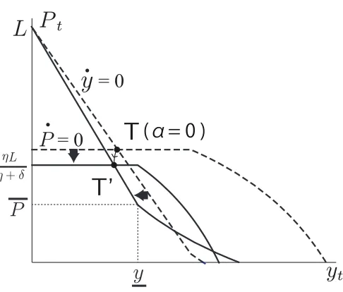
Figure 7: Evolution of income (left) and pollution (right) over generations

incomeyt over the generations:

yt+1=ye(yt)(L−Pt), whereye(yt)≡

          

Ap _ify

t≤y,

Ap(_y+y t

)

/2y ifyt∈(y, y),

As_[ϕθβy

t/(1 +θ)]θ ifyt≥y.

(8)

Let us examine the “limits to growth” of this economy. The ˙yt = 0 locus can be

derived by setting yt+1=yt in equation (8).9 The result is

y∗ (Pt)≡

           [

As_{(ϕθβ/(1 +θ))}θ_(L−P t)

]1/(1−_θ)

≥y ifPt≤P ,

Ap_(2/(L−P

t)−1/(L−P))−1∈(y, y) ifPt∈(P , P),

Ap_(L−P

t)≤y ifPt≥P ,

(9)

where P≡L−y/Ap _{andP ≡(1 +θ)P−θL.}

Figure 7 (left) depicts the ˙y = 0 locus (i.e., function y =y∗

(Pt) in equation 9) in

(y, P) space. The level of income increases over generations if and only if the (y, P)

pair is to the left of this locus. Similarly to Figure 2, the ˙y = 0 locus is downward

sloping. This means that the economy can grow up to a higher level of income when

pollution is lower and, hence, the environment is better. In this economy, this occurs

for two reasons. First, when the environment is better (Pt is lower), the agents have

greater ability to work (ℓt=L−Pt), such that they can produce more output. This

is a direct effect of the environment on income. There is also an indirect effect that

9

Because the model in this section is formulated in discrete time, it is more precise to call it theyt+1=yt

is manifested over the generations: when the environment is better, parents can leave

a larger amount of income to their children, and children themselves also have hige

ablility to learn (ℓt+1=L−Pt+1), both of which enable agents in the next generation

to adopt a better technology. In Figure 7 (left), the effect of the environment on the

technological shift appears when the amount of pollution is betweenP andP. When

Pt is within this range, a marginal changePthas a larger effect on long-term income

through inducing agents to employ the productive (and sustainable) technology in a

larger portion of total production (i.e., the long-run level of st+1 increases with Pt).

This explains why the ˙y= 0 locus is flatter in this segment than in other segments.

3.3

Dynamic interaction between income and environment

We have shown that, given the amount of pollutionPt, the evolution of income is

deter-mined by equation (8). How, then, isPtdetermined? Will it follow the environmental

Kuznets curve? From (4), (5), (7) and ℓt = L−Pt, the evolution of the amount of

pollution in equilibrium can be written as

Pt+1= (1−δ)Pt+η(1−s(yt))(L−Pt), (10)

whereη≡_bηAp_{. Equation (10) shows that the evolution ofP}

tis also determined by the (y, P) pair. By applyingPt+1=Ptfor (10), we obtain the stationary level of pollution

for each given income level yt:

P∗ (yt) =

          

ηL/(η+δ) ifyt≤y,

ηL/(η+δ/σ(y−yt)) ifyt∈(y, y),

0 ifyt≥y.

(11)

Let us call the curve given by (11) the ˙P = 0 locus, as depicted in Figure 7 (right).

The amount of pollution in this economy increases toward the ˙P = 0 locus whenever

the (y, P) pair is below this locus. Observe that the ˙P= 0 locus is (weakly) downward

sloping because a richer economy can afford to invest more in human capital and, hence,

can employ cleaner technologies (recall equation 7), which implies lower pollution in

the long run. Note, however, that the amount of income yt itself changes depending

onPt, and hence we need to examine the dynamic interaction betweenytandPtover

the process of economic development. This can be done by combining the ˙y= 0 locus

and the ˙P = 0 locus in one figure.

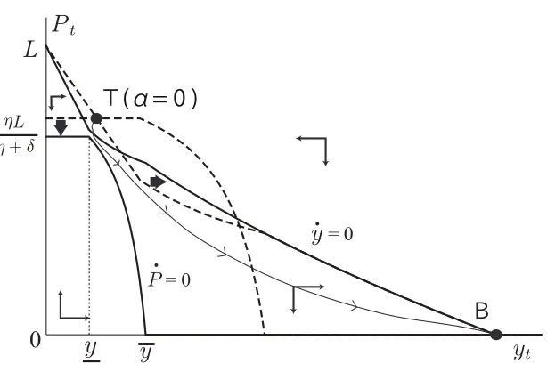
Figure 8 depicts the phase diagram of the dynamic system in (y, P) space.10 We

can observe that there are two stable steady states,T_andB_{, and one saddle point} U_.

10

0

T

U

B

P

L

´L ´+±

y

y

k (EKC) l

m

saddle pa th

(poverty-environment trap)

(unstable)

(better steady state)

y

.

= 0

P

.

= 0

Figure 8: The poverty-environment trap and the environmental Kuznets curve in

equilib-rium

It depends on the initial conditions which steady-state the economy converges to in the

long run. In this system, both yt andPt are state variables, and therefore, the initial

condition is given by a pair of the income of the initial adult generation y0 (i.e., the

parents of generation-0 agents) and the initial amount of pollutionP0.11 Because we

are interested in the process of economic growth, we suppose y0 to be small so that

we can examine the process from the initial stage of development. It will also make

sense to assume the initial amount of pollution P0 to be small if we consider that the

economy starts from a pre-industrial society, but the precise values of P0, as well as

the parameters of the model, will vary across economies.

Figure 8 shows three representative equilibrium paths that start from slightly

dif-ferent initial combinations of (y0, P0). Path k illustrates an equilibrium path when

the economy starts from a low P/Y ratio. On the first half of this path, pollution

gradually accumulates while the output increases. However, once the income level

suf-ficiently rises and the path moves past the ˙P = 0 locus, the accumulated amount of

pollution begins to decrease. This is because the economy now has enough income

to invest in human capital and, therefore, no longer needs to rely as much on dirty

primitive technologies. Thereafter, as the environment improves, the ability (or health

status) of the workers also improves, which enables the income level to increase further

toward the better steady stateB_{. This path explains that the interaction between the}

11

Strictly speaking, the predetermined variables in this system arextandPt. However, becausext=βyt

income level and pollution can endogenously generate the EKC. However, this path is

not the only possibility.

Path lin Figure 8 illustrates another equilibrium path when the economic

devel-opment begins with a higher P/Y ratio. In this case, the economy hits the ˙y = 0

locus (the limits to growth) before encountering the ˙P = 0 locus. This means that the

economic growth has come to its limit due to the environmental degradation, before

the income level reaches the top of the EKC. This is not the end of the story. From

this point, environmental degradation further continues because the economy is still

below the ˙P = 0 curve. After passing the ˙y = 0 locus, the income actually decreases

due to the deteriorated ability of workers who are seriously affected by a poor

en-vironment. The economy eventually converges to steady state T_{, which we call the}

poverty-environment trap. In this trap, workers cannot escape from poverty because

the deteriorated environment lowers their ability and productivity. At the same time,

the economy cannot escape from the deteriorated environment because workers are too

poor to obtain human capital and, hence, cannot employ cleaner technologies. This

mutual causality creates a stagnating economy that suffers both from poverty and a

de-teriorated environment. Pathmin Figure 8 shows the case where the initialP/Y ratio

is even higher. In this case, the economy converges directly to the poverty-environment

trap T_{, which is locally stable and can be approached from any direction in the phase}

diagram.

These two long-term possibilities, the better steady state and the poverty-environment

trap, are grossly different both in terms of environmental quality and income. What,

then, separates the successful economies that get past the peak of the EKC from the

economies that stagnate in the mutual trap of poverty and environmental degradation?

Observe from Figure 8 that there exists a saddle path that converges to the saddle point

U_{. Because both y0 and P0 are predetermined state variables, there is virtually zero}

possibility that the economy happens to be on this path. However, the location of

this saddle path is important because it separates the two long-term outcomes: the

economy converges to the poverty-environment trap if and only if the initial (y0, P0)

pair is above the saddle path. Therefore, even when all parameters are identical, a

slight difference in the initial conditions (which depends on many factors, e.g., whether

a country has been colonized or not and, if so, by what country) may explain persistent

international inequality in income and environmental quality. In addition, if the

pa-rameters of economies are not identical (e.g., because of regional characteristics), the

location of the saddle path as well as the locations of the steady states would differ

across countries. This explains another possible reason why some economies have

from low income and poor environmental conditions, as we have observed in Figure 4.

3.4

Environmental policies for trapped economies

Now let us discuss how environmental policies can or cannot save economies that are

currently trapped in the poverty-environment trap and whether such policies can

mit-igate the international inequality both in terms of income and the environment. We

have explained that, in a trapped economy, the environmental quality and thus the

productivity was low because people rely on the primitive technologies that emit

pol-lution. A direct approach to solve this problem is to limit the use of such technologies,

i.e., to force them to reduce pollution even if it is costly for individuals. Alternatively,

the authorities can tax the use of dirty technologies (or, equivalently, tax emissions)

and use the tax revenue for pollution abatement activities. In either case, the net

income from using the primitive technologyApwill fall,12 but the amount of pollution

per unit output from the primitive technology, given by parameterη, will also fall. To

examine the equilibrium outcome of such policies in a convenient way, we suppose that

both Ap _{andη are functions of the strictness of the environmental policy, denoted by}

α∈[0,1], and that both are decreasing in α.13

Figure 9 illustrates how such environmental policies affect the trapped economy.

Recall that in the poverty-environment trap, both the environmental quality and the

income are low so that Pt > P and yt < y hold. In this region, from (9) and (11),

we can confirm that the ˙y = 0 locus shifts leftward, while the ˙P = 0 locus shifts

downward. This implies that there are two opposing effects of environmental policies

on the income of a trapped economy. First, the leftward shift of the ˙y= 0 locus means

that, given the quality of the environment, the household income declines. This result

comes directly from our assumption that environmental policies that aim to reduce

emissions are costly for individuals. If it takes time for the environmental quality to

change, as assumed in equation (10), then the short-term effect of environmental policy

on income is necessarily negative.

In the long-run, however, the environment improves, as reflected in the downward

shift in the ˙P = 0 locus. With a better environment, the productivity of workers will

improve, increasing their incomes. The long-term net effect of environmental policy

12

Originally we assumedAp _{to be a technology parameter. Here, we reinterpretA}p_{as the productivity}

after deducting the cost of abatement activity or after deducting the environmental tax.

13

Specifically, in Figure 9 we assume that a stricterαreduces the two parameters proportionally:Ap_{(α) =}

(1−α)Ap0andη(α) = (1−α)η0. Equation (10) implies that for a given amount of labor input the increments

T

(α= 0 )

T'

y

= 0

.

P

= 0

.

P

L

y

´L ´+±

P

y

Figure 9: Effect of a small environmental tax or the enforcement of mild pollution reduction

in a trapped economy (a magnified view around steady state

T

_).

diagram without the environmental tax. The solid loci show the case of α= 0.15 (i.e., when bothAP _and

ηare 85% of their original values).

on income depends on the relative magnitude of these two effects. (In other words, it

depends on the relative significance of the reductions in AP _{andη, or more generally,}

it depends on the elasticity of the productivity loss to the reduction of emissions). As

illustrated in Figure 9, the net effect can be negative even in the long-run. The steady

state level of income in steady stateT’ _{under an environmental policy of α= 0.15 is}

lower than the income in steady state T_{withα= 0.}

The above results suggest that it is not easy to form a consensus on the

environmen-tal policy to reduce emissions in a poverty-environmenenvironmen-tally trapped economy because

it will further undermine the already low income in the short run, and it is not certain

whether it will raise income even in the long-run. However, a sufficiently strong

envi-ronmental policy can have quite different implications. As illustrated by Figure 10, the ˙

P = 0 and ˙y = 0 loci become detached from each other whenαis large enough. This

means that the poverty-environmental trap no longer exists in the new phase diagram,

and because of this structural change the economy necessarily converges to the now

unique steady state B_{. In this transition, the environment improves simultaneously}

with the rising income, as in the latter half of the EKC.

Why does a strong environmental policy give rise to such a drastic change? One

possible reason is that a better environmental quality improves the productivity and,

0

T

B

P

L

´L ´+±

y

y

y

= 0

.

P

= 0

.

y

(α= 0 )

Figure 10: Effect of a large environmental tax or the enforcement of large pollution

reduc-tion in a trapped economy.

the case ofα= 0.27 (i.e., when bothAP _{andηare 73% of their original values).}

cleaner technologies. However, as we have explained above, environmental policies to

reduce emissions do not necessarily improve income as long as individuals are relying

on dirty primitive technologies (i.e., when Pt > P and yt < y), and therefore, this

first cause does not always work. The second and more definite cause of the structural

change is that because a strong environmental policy reduces the private returns from

adopting primitive technologies, workers are induced to invest in human capital and

adopt cleaner technologies even at lower income levels. This can be confirmed by the

fact that the threshold levels of income for education,y andy in equation (7), become

smaller when Ap _falls.14 _{Obviously, such a policy temporarily reduces the income of}

poor households (given that the environmental quality does not change instantly). As

time passes, however, the environment improves gradually, which increases productivity

and income. Once the income level passes a threshold level (specifically, whenytand

Pt pair falls below the saddle path in Figure 8), workers are now willing to invest in

human capital and cleaner technologies even without further policy interventions, and

the economy autonomously improves toward the better steady state.

To summarize, once an economy falls into the poverty-environment trap, it is

dif-ficult to build a consensus on environmental policies because such policies are likely

to worsen income and welfare, at least temporarily. In addition, when the policy

in-tervention is insufficient, poverty can be aggravated even in the long run. However,

14_{Recall thatσ}

the situation can be solved permanently if a sufficiently strong environmental policy

is continued for a certain period until the economy reaches the autonomous process of

economic growth and environmental improvements. Given the short-term cost of such

a drastic intervention, assistance from developed economies (e.g., by providing funds

for the abatement cost, subsidies for education, or income assistance for households

whose earnings are adversely affected by environmental policies) will certainly be a key

in helping economies escape from the poverty-environment trap, thereby reducing the

wide international inequality both in incomes and environmental quality.15

4

Sustainability of long-term growth under global

warming

In the previous section, we examined the problems of large international differences in

income and environmental quality. We showed the possibility that the interaction

be-tween the environment and growth within each country creates a poverty-environment

trap and that this mechanism can explain the long-lasting international inequality in

terms of both environmental quality and income. Now, let us turn to the growth of the

world economy as a whole and examine how can it be harmonized with the global

envi-ronment, particularly regarding the problem of global warming. As we have discussed

in the latter half of Section 2, the growing world economy emits increasing amounts of

global warming gases, which is suspected to intensify the risk of natural disasters. The

aggregate economic damage from natural disasters, which mostly takes the form of the

destruction of capital stocks, has been increasing at a speed faster than the growth of

the world GDP (see Figure 5). If this trend continues, the risk of losing the capital

stock will sooner or later exceed a threshold at which the economy does not want to

invest further in capital stock. This is the “limits to growth” for the world economy

(see path fin Figure 6). Can any environmental policy prevent such a situation from

occurring and sustain long-term growth? Based on a simplified version of the

endoge-nous growth model by Ikefuji and Horii (2012), this section presents a formal model of

emissions, natural disasters, and the “limits to growth.”

15

4.1

A model with global pollution and capital destruction

While the previous section considered only human capital, in this section, we consider

explicitly the accumulation of physical and human capital. Note that the damage from

natural disasters occurs most strikingly in the form of capital destruction. In addition,

natural disasters entail many human casualties and therefore destroy a substantial

amount of skills and knowledge (i.e., human capital). A knowledge based economy

with a large stock of human capital can be vulnerable to natural disasters once its

telecommunication network is damaged. Therefore, it is appropriate to develop a model

where the economy accumulates both physical and human capital and where both are

subject to the risk of natural disasters. This specification also allows us to examine the

properties of long-term economic growth, rather than one-time transitional dynamics

from a poor to a rich economy.16

However, considering two types of capital simultaneously makes the analysis

sub-stantially complex. Therefore, we make several innocuous simplifications. First, rather

than explicitly considering different generations (youth and adults, as in the

previ-ous section), let us consider a representative hprevi-ousehold and assume that they divide

their human capital (or their disposable time) between production (fraction ut) and

education (1−ut). In addition, rather than considering the choice between the two

technologies, we suppose that production always uses fossil fuelsPtthat cause the

emis-sion of greenhouse gases of the same amount Pt, but that it is possible to adjust the

amount of such an input in the production process. The output of the world economy

is then given by a constant-returns-to-scale production function:

Yt=AKtα(utHt)1 −α−β

Ptβ, (12)

where Kt and Ht are the aggregate amounts of physical and human capital,

respec-tively. It is possible to interpret that the primitive technology in the previous section

corresponds to the situation where the economy uses a large amount ofPtwhile

mak-ing little use ofHt. Sustainable technology corresponds to the opposite combination.

Because this section’s objective to examine how the economy’s reliance on fossil fuels

Ptlimits the possibility of sustained growth through global warming and increased risk

of natural disasters, we do not explicitly consider the finiteness of such resources.17

16

While classical growth models requires exogenous technological change to explain long-term growth, the literature on endogenous growth (with a seminal study by Lucas 1988) has shown that long-term growth can be explained within a model if we consider both physical and human capital accumulations simultaneously.

17

We also simplify the process of education. When the representative household

uses amount (1−ut)Ht of their human capital for education, it produces additional

B(1−ut)Ht units of new human capital, where B is a constant parameter for the

efficiency of education (see equation 14 below).

In the model of the previous section, we assumed that local pollution reduces the

productivity (ability) of agents. Instead, we now assume that global pollution (i.e.,

the emission of greenhouse gases) raises the risk of capital stock destruction. Suppose

that when the world economy emits amountPtof greenhouse gases, then, on average,

a fraction ϕPt of physical capital is destroyed by natural disasters within a year.18

Natural disasters will also erode a fraction ψPt of human capital, where we assume

0 < ψ < ϕ.19 _{Then, the aggregate amounts of physical and human capital evolve}

according to

˙

Kt = Yt−Ct−(δK+ϕPt)Kt, (13)

˙

Ht = B(1−ut)Ht−(δH+ψPt)Ht, (14)

where δK and δH are depreciation rates of physical and human capital, respectively,

excluding the effect of global warming. Because we are concerned about long-term

growth rather than short term fluctuations caused by individual events of natural

disasters, we simply assume that the whole economy consists of many regions, and, by

the law of large numbers, there is no aggregate uncertainty on the aggregate damage in

each year. In this setting, the use of fossil fuelsPtin effect accelerates the depreciation

of capital through the larger damages caused by natural disasters.

The representative household has the standard CRRA utility function:

∫ ∞

0

C1−θ −1 1−θ e

−ρt

dt. (15)

Let us consider a market economy where the authorities levy a per-unit tax ofτ >0

on the use of fossil fuelsPt(or, equivalently, the amount of greenhouse gas emissions).

Here, we abstract from the international politics and assume that the whole economy

(i.e., the world’s economy) can set a common rate of environmental tax.20 _Suppose

the markets are perfectly competitive and there is a representative firm that produces

18

For simplicity, we do not explicitly consider the accumulation of greenhouse gases in the atmosphere. Ikefuji and Horii (2012) show that the basic property of the result is the same when we explicitly consider the accumulation process.

19

While human and physical capital are vulnerable to natural disasters, it is reasonable to think that physical capital suffers more directly from natural disasters and, therefore, that the damage fraction of physical capitalφPtwould be larger than that for human capitalψPt.

output Yt according to (12). Let the price of the output be normalized to one, and

assume that there are no other costs of usingPtother than the environmental taxτ.21

Then, the first order condition for the profit maximization implies

Pt=βYt/τ. (16)

Equation (16) clearly shows that the emission of greenhouse gases Pt increases

proportionally with the world’s GDP,Yt, if there is no strengthening of environmental

policyτ. At the same time, this equation shows that emissionPtcan be reduced if the

environmental tax rate τ is raised, confirming the discussion in section 2. However,

this does not come without a cost. By substituting (16) into production function (12),

we see that output can be expressed as

Yt=

( ˜

Aτ− β

1−β

)

Kαb

t(utHt)1−αb, (17)

where ˜A≡ββ/(1−β)

A1/(1−β)

and αb≡α/(1−β). Equation (17) can be interpreted as

the aggregate production function given the level of environmental tax τ. It has the

form of a standard Cobb-Douglas function with two inputs,KtandutHt, and its total

factor productivity (TFP) is given by ˜Aτ−β/(1−β)

. This expression clearly shows that,

given the current amounts of physical and human capital, the environmental tax lowers

the productivity.

4.2

“Limits to growth” under constant tax rate

We first show that if the environmental tax rate τ is kept constant, the interacting

processes of economic growth and environmental degradation eventually lead to the

“Limits to growth.”

In this economy, the only source of externality isPt, which represents the use of

fossil fuels and, hence, the accompanying emission of greenhouse gases. Other than

this aspect, the conditions for the market equilibrium with the representative household

and the representative firm coincide with the conditions for the welfare maximization

problem.22 _{The problem is to maximize the utility (15) subject to the production}

levels and geography, it is not easy to agree on a common standard for greenhouse gas emissions, and it will be even more difficult to strengthen it over time. As we will see, such conflicts in international politics will create a threat to the sustainability of the world’s economic growth.

21

In the present setting, we assume that the tax revenue is returned to the household in a lump sum fashion. With a minor modification of the model, it is possible to interpret that τ includes other costs of using fossil fuels, such as extraction costs. In this case, only the remaining fraction ofτ will be returned to households.

function (12) and the resource constraints (13) and (14), where we take the evolution

ofPtin (16) as given. By setting up a Hamiltonian, we obtain the following first order

conditions for this problem, which should also hold in the market equilibrium:

˙

Ct

Ct = 1

θ

[(

αYt Kt

−δK−ϕPt

) −ρ

]

, (18)

˙

Ht

Ht+ ˙

ut

ut

−Y˙t

Yt = (B

−δH−ψPt)−

(

αYt Kt

−δK−ϕPt

)

. (19)

Equation (18) is the Euler equation for the intertemporal consumption. Note that

the term (αYt/Kt−δK−ϕPt) in the right-hand side (RHS) represents the (expected)

rate of return from physical capital investment, i.e., the marginal product of capital

αYt/Ktminus the depreciation rateδK minus the expected loss from natural disasters

ϕPt. Recall from (16) that if the environmental tax rateτis constant and the economic

growth continues ( ˙Yt>0), the representative firm uses an ever increasing amount of

fossil fuels Pt. The resulting increase in the risk of natural disasters lowers the rate

of return from physical capital investment (αYt/Kt−δK−ϕPt). Equation (18) shows

that economic growth can be sustained ( ˙Ct/Ct > 0) only when the rate of return

from physical capital investment is kept above the rate of time preference,ρ. For this

condition to hold along economic growth, the continual rise in the expected damage

ϕPtmust be offset by an increase in the marginal product of physical capitalαYt/Kt.

Will such an increase inαYt/Ktactually occur? Note that under production

func-tion (17) the marginal product of physical capitalαYt/Ktrises when the economy uses

more human capital utHt relative to the amount of output Yt. The rate of change in

this ratio, utHt/Yt, is represented by the left-hand side (LHS) of equation (19). The

first term in the RHS, (B−δH−ψPt), represents the rate of return from investing in

human capital. The second term is the rate of return from physical capital investment,

as explained above. Therefore, equation (19) shows that the household uses more

hu-man capital in production if the rate of return from huhu-man capital investment is higher

than that from physical capital investment.

As the amount of emissionPt increases in the RHS of (19), the rate of return for

physical capital falls more rapidly than that for human capital (recall that ϕ > ψ),

and therefore, the economy increases its reliance on human capital. This is

consis-tent with the empirical findings of Skidmore and Toya (2002), who suggested that

a higher frequency of climatic disasters leads to a substitution from physical capital

investment toward human capital. This substitution process actually increases the

world’s income

P

^

greenhouse

gas emissions

Y=0

.

Y

P

initial

status

(Limits to Growth)

low

τ

int

erm

edi

ate

τ

high

τ

A

B

C

D

Figure 11: Evolution of the global environment and the world’s income under different

environmental tax rates.

marginal product of physical capitalαYt/Kt, which encourages growth. However, this

process cannot perpetually sustain economic growth under a constant tax rate. As

we discussed, Euler equation (18) implies that nonnegative growth in consumption

re-quires the rate of return from physical capital (αYt/Kt−δK−ϕPt) to be at least ρ.

However, as Pt= βYt/τ rises with economic growth, the rate of return from human

capital investment (B−δH−ψPt) will eventually fall toρ. This means that the RHS

of (19) becomes zero (or negative), and substitution from physical capital to human

capital stops. This means that αYt/Kt cannot rise further, and therefore, the rate

of return from physical capital investment (αYt/Kt−δK−ϕPt) must eventually fall

until it reaches the rate of time preference ρ. At this point, people are unwilling to

invest further in physical capital to increase their consumption, and economic growth

comes to an end.

By setting time derivatives to zero in equations (18) and (19), we find that this

steady state, or the “limits to growth,” is reached when the amount of emissions

increases up to

b

P =B−δH−ρ

ψ . (20)

Figure 11 illustrates the processes of economic growth in (Y, P) space for three

different environmental tax rates. These three paths start from the same level of

capital accumulation. However, as we have shown in equation (17), the initial amount

the higher tax rate reduces the effective TFP. When the tax rate is higher, the initial

level of emissionPt=βYt/τ is also lower due to both higherτ and lower initialYt.

As the economy grows, the amount of emission Pt increases proportionally with

output Yt. Observe from the figure that the slope of the path, Pt/Yt =β/τ, is less

steep when the tax rate is higher. This means that the level of income at which the

economy reaches the “limits to growth” (i.e., when Pt reaches Pb) is proportionally

related to the environmental tax rate:

b

Y = τ

βψ(B−δH−ρ). (21)

Therefore, although a higher environmental tax initially corresponds to a lower output,

it also implies there remains larger room for economic growth.

While Figure 11 illustrates the existence of the limits to growth of the world

econ-omy under a constant environmental tax rate, it also suggests that economic growth

can be maintained if the environmental tax rate is continually raised. Whenever the

world economy reaches the limit of growth, it is possible to bring the economy to a

less steep path of growth that leads to a higher long-term level of output, although

output temporarily falls (e.g., from point A_{to point} B_{, or from point}C_{to point} D_in

Figure 11). It might be even better to raise the environmental tax before the

emis-sion Pt reaches Pb because doing so will allow the possibility of keeping the rates of

return from physical and human capital investment higher, thereby encouraging faster

capital accumulation. However, it is not always better to raise the environmental tax

faster because it lowers the effective productivity of production. In the next

subsec-tion, we examine the desirable environmental tax policy both in terms of the long-term

economic growth rate and in terms of welfare.

Before leaving this subsection, let us explain the difference between Figure 6 and

Figure 11. While we discussed in Section 2 that the ˙Y = 0 locus would appear to

be downward sloping (see Figure 6), the ˙Y = 0 locus we derived so far (Figure 11)

is actually horizontal because Pb = (B−δH −ρ)/ψ does not depend on the income

levelYt. This result is due to several simplifications. In particular, we simply assumed

that δH and ψ do not change with the income level or the level of human capital.

At the initial stage of economic growth, however, when production relied more on

basic labor than advanced human capital, we may interpret thatδH andψ must have

been smaller. As the economy develops and the aggregate human capital accumulates

(i.e., the development of complex systems of skill, knowledge and information in the

world economy), the depreciation or the obsolescence of existing human capital will

accelerate (i.e., δH increases). In addition, as the system of human capital becomes

we incorporate these changes into the model, the ˙Y = 0 locus (Pb= (B−δH−ρ)/ψ)

will become downward sloping, as depicted in Figure 6.

Note, however, that if we do not expect δH and ψ to rise indefinitely, they will

converge to certain constants in the very long run. Because this section examines

the long-run consequences of the interaction between the environment and economic

growth, we consider the situation where economic development has already sufficiently

advanced so that δH and ψ can be seen as constants. In Figure 6, this corresponds

to the region where Yt is sufficiently large that the ˙Y = 0 comes close to the dashed

horizontal line atPt=Pb.

4.3

Environmental policy and sustained growth

In the previous subsection, we confirmed that economic growth can be sustained only

when the environmental tax rate is continually raised. Now let us define the rate of

tax increase gτ≡τ˙t/τtand examine how it determines the long-term rate of economic

growth g∗

≡Y˙t/Yt.23

The long-term rate of economic growth g∗

cannot be higher than the rate of tax

increase,gτ, because otherwisePt=βYt/τtwould continue to increase and eventually

face the “limits to growth,”Pb. Therefore, sustained growth (g∗

>0) requires a positive

rate of environmental tax increase. Under such a policy, there are two possible outcomes

in the state of the environment. If the long-term economic growth occurs at the

same rate as the tax increase (i.e., g∗

= gτ), then the growth rate of Pt = βYt/τt

will become zero, and therefore, the amount of emissions will converge to a constant,

which we denote by P∗

. Another possibility is that output grows slower than the tax

rate (g∗

< gτ). In such a scenario, the amount of emission Pt =βYt/τt falls at the

rate of gP = g∗−gτ < 0 and will converge toward zero. That is, the emissions are

asymptotically eliminated in the long run;P∗ = 0.

In either case, the amount of emissions and, hence, the risk of natural disasters

converge to a constant level. This by itself should be good for economic growth.

However, when the tax rateτis continually increased, is it possible to maintain output

growth, given that a higherτ reduces the effective productivity? Calculating the rates

of change on both sides of equation (17), we find that the growth rate of human capital

gH ≡H˙t/Ht should be higher than the output growth so that it offsets the effective

23

Strictly speaking, because we are interested in the long-term rate of economic growth, not the growth rate in the transition, the precise definition of g∗ _{should be}

≡limt→∞Y˙t/Yt, and it should be called the