http://wrap.warwick.ac.uk
Original citation:
Farsad, Nariman, Guo, Weisi, Chae, Chan-Byoung and Eckford, Andrew W. (2015)
Stable distributions as noise models for molecular communication. In: IEEE Global
Communications Conference (GLOBECOM 2015), San Diego, 6-10 Dec 2015
Permanent WRAP url:
http://wrap.warwick.ac.uk/70463
Copyright and reuse:
The Warwick Research Archive Portal (WRAP) makes this work by researchers of the
University of Warwick available open access under the following conditions. Copyright ©
and all moral rights to the version of the paper presented here belong to the individual
author(s) and/or other copyright owners. To the extent reasonable and practicable the
material made available in WRAP has been checked for eligibility before being made
available.
Copies of full items can be used for personal research or study, educational, or not-for
profit purposes without prior permission or charge. Provided that the authors, title and
full bibliographic details are credited, a hyperlink and/or URL is given for the original
metadata page and the content is not changed in any way.
Publisher’s statement:
“© 2015 IEEE. Personal use of this material is permitted. Permission from IEEE must be
obtained for all other uses, in any current or future media, including reprinting
/republishing this material for advertising or promotional purposes, creating new
collective works, for resale or redistribution to servers or lists, or reuse of any
copyrighted component of this work in other works.”
A note on versions:
The version presented here may differ from the published version or, version of record, if
you wish to cite this item you are advised to consult the publisher’s version. Please see
the ‘permanent WRAP url’ above for details on accessing the published version and note
that access may require a subscription.
Stable Distributions as Noise Models for Molecular
Communication
Nariman Farsad
1, Weisi Guo
2, Chan-Byoung Chae
3, and Andrew Eckford
11 Department of Electrical Engineering and Computer Science, York University, Canada. 2 School of Engineering, University of Warwick, Coventry, UK.
3 School of Integrated Technology, Yonsei University, Korea.
Corresponding Email: [email protected].
Abstract—In this work, we consider diffusion-based molecular
communication timing channels. Three different timing channels are presented based on three different modulation techniques, i.e., i) modulation of the release timing of the information particles, ii) modulation on the time between two consecutive information particles of the same type, and iii) modulation on the time between two consecutive information particles of different types. We show that each channel can be represented as an additive noise channel, where the noise follows one of the subclasses of stable distributions. We provide expressions for the probability density function of the noise terms, and numerical evaluations for the probability density function and cumulative density function. We also show that the tails are longer than Gaussian distribution, as expected.
Index Terms—Molecular Communication, Channel Models,
Noise Models, L´evy Distribution, Stable Distributions.
I. INTRODUCTION
Molecular communication is a biologically inspired form of communication, where chemical signals are used to transfer information [1]. It is possible to modulate information on the information particles using different techniques such as: concentration [2], type [3], number [4], or time of release [5]. Moreover, information particles can propagate from the transmitter to the receiver using diffusion [6], active transport [7], bacteria [8], and flow [9]. Recently the possibility of molecular communication has been demonstrated using a tabletop experimental setup [10], [11].
We consider diffusion-based molecular communication, where information is encoded on the time of release of molecules. Timing channels for diffusion-based molecular communication were first proposed in [5]. A molecular com-munication timing channel based on additive inverse Gaussian distributed noise for flow induced channels was presented in [12], and tight bounds for the capacity of this channel was presented in [13]. In [14], a special type of timing modulation, where the order of release of consecutive molecules of differ-ent type is used to encode information is proposed. The time interval between release of two consecutive release of large number of information particles is proposed as a modulation scheme in [15].
In this work we propose three general classes of timing channels for diffusion-based molecular communication: the regular timing channel, where information is encoded in the release timing of information particles (channel A); time
between release modulation using the same type of infor-mation particles, where the inforinfor-mation is encoded in the time between release of two consecutive particles of the same type (channel B); and time between release modulation using different types of information particles (channel C). In all three cases it is demonstrated that the channel can be reduced to an additive noise channel where the noise term falls in the stable distribution family [16]. In particular, for channel A the noise follows the well-known L´evy distribution.
Stable distributions have been used in a number of fields to model noise. In [17], alpha-stable distributed noise was used to create a more realistic noise model for room acoustic channels. In radio communications, symmetric alpha-stable distributions were used to model impulsive non-Gaussian noise that exists in some systems such as ultra-wide bandwidth (UWB) systems [18], [19]. Capacity bounds for a special class of alpha-stable additive noise channels had been provided in [20], [21].
There are only three classes of stable distribution with closed-form expressions for the probability density function (PDF) in term of elementary functions: Gaussian, Cauchy, and L´evy. In this work, we derive closed-form expressions for the PDF of the noise terms in our channels in terms of the complex error function and Voigt functions [22], which are used in other fields of science such as physics. We numerically compare the stable-distributed noise densities and distribution functions to the Gaussian distribution, and show that the stable distribution exhibits longer tails. We present expressions for the asymptotic tail probability of the noise models and show that the expressions converge to the actual tail probabilities quickly.
The rest of this paper is organized as follows. In Section II we present three timing channel models for diffusion-based molecular communication. We then derive the PDF for the additive noise term in each channel model in Section III. Nu-merical evaluations of the PDF and the cumulative distribution function are presented in Section IV, and expressions for the tail probabilities are provided. The concluding remarks are presented in Section V.
II. TIMINGCHANNELMODELS
we assume that there is no inter-symbol interference. First, we consider the timing channel proposed in [12], [23], where the information is encoded in the release timing of a single information particle. Let Tx be the release timing of the information particle, and Ty be the time of arrival at the receiver. Then we have
Ty=Tx+Tn, (A) whereTn is the random propagation delay of the information particle. Tn is parametrized by the distance between the transmitter and the receiver and the diffusion coefficient of the information particle.
One of the main challenges of this propagation scheme is the need for synchronization between the transmitter and the receiver. To overcome this challenge, time between release modulation (TBRM) could be used, where information is encoded in the time duration between two consecutive release of molecules. Two cases are possible: either the two released information particles are the same, or the two released infor-mation particles are different.
First, we consider the case where both information particles are the same. LetTx1 be the release timing of first information particle andTx2 be the release timing for the second informa-tion particle with Tx2 > Tx1. We assume the information is encoded in Lx = Tx2 −Tx1. Then using (A), the channel model for this modulation scheme is given by:
|Ty2−Ty1|=|Tx2−Tx1+Tn2−Tn1|,
Ly=|Lx+Ln|, (B) whereLn=Tn2−Tn1 is the random noise andTn2 andTn1 are independent and identically distributed noise terms in (A). Another modulation scheme is when two different types of information particles are used. Let Txa be the release timing
of type-ainformation particle and Txb be the release timing
for the type-binformation particle. We assume the information is encoded inDx=Txb−Txa. Unlike (B) whereLxis always
positive, in this caseDxcan be positive or negative depending on the order that type-aand type-b information particles are released. Using (A), the channel model for this scheme is given by:
Tyb−Tya=Txb−Txa+Tnb−Tna,
Zy=Zx+Zn, (C) whereZn=Tnb−Tna is the random noise andTnb andTna
are independent noise terms in (A).
III. TIMINGCHANNELNOISEMODELS
In this section, we will find the probability density function of the noise terms Tn,Ln, and Zn and discuss some of the properties of these random variables.
A. Channel A
First, we consider the channel in (A) and the random propagation noise term Tn. If we assume that the receiver is absorbing the information particles, which is the case for
many practical applications,Tn is distributed according to the first hitting time distribution. In previous works, it was shown that the first hitting time for the flow induced diffusion in 1-dimensional (1D) space follows Inverse Gaussian distribution [12]. In this work, we consider the diffusion channel with no flows. In this case,Tn is a L´evy distributed random variable. The probability density function (PDF) of a non-negative L´evy-distributed random variableX is given by
f(x;µ, c) =
r c
2π(x−µ)3exp
− c
2(x−µ)
, (1) where µ and c are parameters of the L´evy distribution. The characteristic function for a L´evy distributed random variable is given by
ϕ(t;µ, c) = expjµt−p
−2jct, (2) wherej=√−1is the imaginary number. We use the notation
∼L´evy(µ, c)to represent a L´evy distributed random variable with parameters µ and c. Using this notation the additive noise is given by Tn ∼L´evy(0, d
2
2D), whered is the distance between the transmitter and the receiver andDis the diffusion coefficient. Therefore, we have
fTn(tn) =
d
p
4πD(tn)3exp −
d2
4Dtn
!
, (3)
Similarly, the conditional PDF P(Ty|Tx) ∼ L´evy(Tx, d 2
2D). The L´evy distributed noise holds for 1D diffusion and also for 3D diffusion with a spherical absorbing receiver with an scaling parameter [1], [24].
B. Channel B
To find the noise distribution for the channel in (B), we consider a class of probability distributions known as stable distributions [16], [25]. The L´evy distribution is a part of stable distributions.
Definition 1. A random variableXhas a stable distribution if for two independent copiesX1andX2, and positive constants
a,b,c, andd∈Rthe following holds
aX1+bX2
d
=cX+d,
where=d is equality in distribution.
Generally, stable distributions are defined by their charac-teristic function
ϕ(t;µ, c, α, β) = exp
jµt− |ct|α(1−jβsgn(t)Φ)
, (4) wheresgn(.) is the sign function (i.e. sign oft),−∞< µ <
∞,c≥0,0< α≤2,−1≤β≤1, and Φ =
(
tan(πα/2) ifα6= 1
−2
πlog(|t|) ifα= 1
distribution with parametersµ,c,α, andβ. The following are some of the important properties of stable distributions.
Property 1. If a random variable X ∼ S(µ, c, α, β), and random variable
Y =X−µ
c ,
thenf(x)dx=f(y)dy, andY is the standard form ofX.
Property 2. Stable random variables with β = 0 have symmetric PDFs.
With these definitions we now model the noise term Ln in (B).
Theorem 1. The characteristic function for the noise termLn
is given by
ϕ t;
√
2d
√
D
!
= exp
"
− √
2d
√
D
p
|t|
#
,
where d is the distance between the transmitter and the receiver and D is the diffusion coefficient of the information particle. Therefore,Ln ∼ S(0,2d
2 D ,
1 2,0).
Proof. Since Ln = Tn2 + (−Tn1) with Tn2, Tn1 ∼
S(0, c,12,1), where c = 2dD2. Since Tn1 and Tn2 are inde-pendent, the characteristic function for Ln is given by
ϕLn(t) =ϕTn2(t)ϕTn1(−t) (6) = exph−p|ct|(1−jsgn(t))i×
exph−p|ct|(1 +jsgn(t))i (7) = exph−p|4ct|i (8)
Only the PDFs of three classes of stable distributions are known to have closed-form expressions in terms of elementary functions: the Gaussian distribution with α = 2 (the value of β does not matter in this case and can be assumed to equal zero), the L´evy distribution with α= 0.5 andβ = 1, and Cauchy distribution with α = 1 and β = 0. To find an expression for the PDF of the noise term Ln in (B), we use Property 1, and define the PDF for the standardized distribution with 2Dd2 = 1. Using Property 1, the standard PDF could be used to calculate probabilities involving non-standard random variables just like the way the standard Gaussian PDF could be used to calculate probabilities involving non-standard Gaussian random variables.
The PDF of the standardized stable distribution can be represented by the integral [26]
f(x;α, β) = 1
π
Z ∞
0
e−tαcos[xt+βtαΦ], (9) whereΦis given in (5). This integral reduces to [26]
f(x; 1/2, β) =<
z πx[
√
πe−z2−2jF(z)]
, (10)
where
F(z) =e−z2
Z z
0
et2dt (11) is the Dawson’s Integral [27], and
z= 1 +β−j(1−β)
2√2x . (12)
It is possible to rewrite (10) in terms of the complex error function, also known as Faddeeva function or the Kramp function [27]
w(z) =e−z2
1 +√2j
π
Z z
0
et2dt
=e−z2erfc(−jz), (13) whereerfc(.) is the complementary error function. Using the relation [27]
F(z) = 0.5j√π(e−z2−w(z)), (14) and the propertyw(−z) = 2e−z2
−w(z), we can rewrite (10) as
f(x; 1/2, β) =<
z
√
πxw(−z)
. (15) One of the benefits of writing the PDF in terms of the complex error function is that there are a large body of work that considered calculating it numerically. Moreover, ifz=a+jb, for b >0 the complex error function can be represented by its real and imaginary parts as
w(a+jb) =K(a, b) +jL(a, b), b >0, (16) where
K(a, b) = √1
π
Z ∞
0
exp(−t2/4) exp(−bt) cos(at), b >0 (17)
and
L(a, b) = √1
π
Z ∞
0
exp(−t2/4) exp(−bt) sin(at), b >0 (18)
are the real and imaginary Voigt functions which are used widely in many fields of physics, astronomy, and chemistry and can be computed numerically.
Using Property 2, the probability density function of Ln is symmetric. Therefore, the probability density function for
Ln≥0 is sufficient for characterizing the PDF. Sinceβ = 0, when Ln > 0 we can write z = pln−jpln where pln =
1/√8ln. Using (15)-(18) the standardized noise termLnwhen
Ln≥0 has the PDF
f(ln) =
1 √
8πl3
n
K(−pln, pln) +L(−pln, pln)
ln>0
2
π ln= 0
,
(19)
C. Channel C
The channel noiseZngiven in (C) can be different fromLn since two different types of information particles can be used with different diffusion coefficients. Let Da be the diffusion coefficient of information particle a andDb be the diffusion coefficient for the information particle b. Also, without loss of generality assume particle a is released first followed by particleb. We now model the noise termZn in (C).
Theorem 2. The characteristic function for the noise termZn
is given by
ϕ t;d( √
Da+
√
Db)2
√ 2DaDb
,
√
Da−
√
Db
√
Da+
√ Db ! = exp −
d(√Da+
√
Db)2
√ 2DaDb
p
|t| 1−j
√
Da−
√
Db
√
Da+
√
Db
sgn(t) !
,
where d is the distance between the transmitter and the receiver and Da and Db are the diffusion coefficient of the
information particles. Therefore,
Zn ∼ S 0,
d(√Da+
√
Db)2
√
2DaDb
,1
2,
√
Da−
√
Db
√
Da+
√
Db
!
.
Proof. Since Zn = Tnb + (−Tna) with Tna, Tnb ∼
S(0, ci,12,1), where ci = √2dD
i for i ∈ {a, b}. Since Tna
andTnb are independent, the characteristic function forZn is
given by
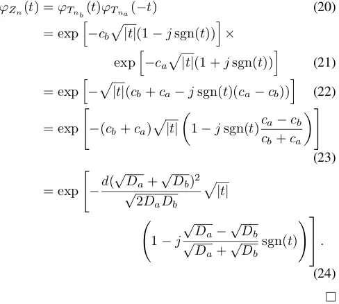
ϕZn(t) =ϕTnb(t)ϕTna(−t) (20)
= exph−cb
p
|t|(1−jsgn(t))i×
exph−ca
p
|t|(1 +jsgn(t))i (21) = exph−p
|t|(cb+ca−jsgn(t)(ca−cb))
i
(22)
= exp
"
−(cb+ca)
p
|t|
1−jsgn(t)ca−cb
cb+ca
#
(23)
= exp
"
−d( √
Da+
√
Db)2
√
2DaDb
p
|t|
1−j
√
Da−
√
Db
√
Da+
√
Db sgn(t)
! .
(24)
When the diffusion coefficients of the two particles are almost equal,Znhas the same distribution asLn (i.e.β= 0). When√Da
√
Daor
√
Da
√
Da,β =±1and henceZn is L´evy distributed. Therefore, channel (C) can be reduced to channel (A), when one information particle has a much higher diffusion coefficient than the other, with the added benefit that no synchronization is required between the transmitter and the receiver.
For the general case, we haveβ = (√Da−
√
Db)/(√Da+
√
Db). We can write (12) asz=px−jqxwhenx >0, where
px= (1 +β)/(
p
8|x|)andqx= (1−β)/(
p
8|x|). Similarly, we can write (12) asz=−qx−jpxwhenx <0. Then using (15) and the Voigt functions decomposition of the Faddeeva function (17) and (18) the PDF of the standardized distribution is given by
f(zn;β) =
1 √
8πz3
n
(1 +β)K(−pzn, qzn)
+ (1−β)L(−pzn, qzn)
, zn>0
2(1−β2)
π(1+β2)2, zn= 0
1 √
8π|zn|3
(1−β)K(qzn, pzn)
−(1 +β)L(qzn, pzn)
, zn<0
,
(25)
where the second term follows from [25].
IV. NUMERICALEVALUATION ANDTAILPROBABILITIES
[image:5.612.58.302.389.608.2]As was shown in the previous section, it is possible to write the PDF for the noise terms in channel (B) and (C) in terms of real and imaginary Voigt functions. These functions can be numerically calculated using efficient algorithms such as [28]. Moreover, for the case of general stable distributions with any parametersµ, c,α, andβ it is possible to calculate the PDFs and the cumulative distribution functions (CDF)s numerically using the fast Fourier transform or by numerically solving definite integrals [29]. In this section, we plot the PDF and CDF of the noise terms of channels (A-C) and compare the PDF to the Gaussian PDF, which is typically assumed in the literature.
Fig. 1 shows the PDF of standardized stable distribution noise terms in channels (A)-(C), as well as the standard Gaussian distribution. As can be seen from the plots, the PDF of the noise terms in all three channels are very different from Gaussian noise. The peaks in the PDF tend to be narrower, while the tails tend to be longer. Moreover, as can be seen the larger the parameterβ the more asymmetric the PDF. For
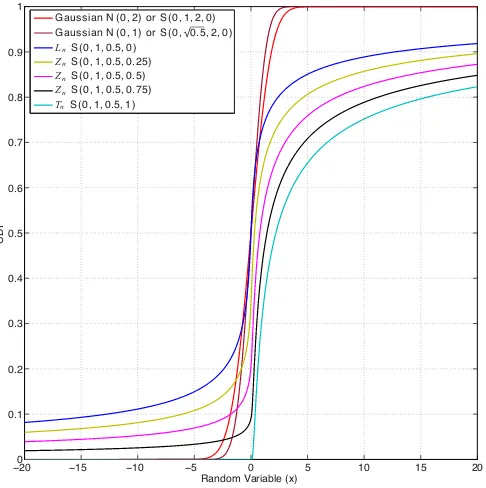
β = 1 the PDF is the standard L´evy distribution which is non-zero only for positive values. The cumulative distribution function (CDF) of the standardized stable distributions are shown in Fig. 2. Again it can be seen that each distribution is quite different and that non-Gaussian stable distributions exhibit long tails.
To compare the tails of each distribution, we use the asymptotic approximation presented in [30]. In particular, if
X is a standardized stable random variable with parameters 0< α <2 andβ, then asx→ ∞,
P(X > x;α, β)≈1 +β
πxα Γ(α) sin
απ
2
−50 −4 −3 −2 −1 0 1 2 3 4 5 0.1
0.2 0.3 0.4 0.5 0.6 0.7
Random Variable (x)
PD
F
Gaussian N (0, 2) or S(0, 1, 2, 0) Gaussian N (0, 1) or S(0, √0.5, 2, 0)
LnS(0, 1, 0.5, 0)
ZnS(0, 1, 0.5, 0.25)
ZnS(0, 1, 0.5, 0.5)
ZnS(0, 1, 0.5, 0.75)
[image:6.612.317.558.55.303.2]TnS(0, 1, 0.5, 1)
Fig. 1. The probability density function of different standardized stable distributions.
−200 −15 −10 −5 0 5 10 15 20
0.1 0.2 0.3 0.4 0.5 0.6 0.7 0.8 0.9 1
Random Variable (x)
C
D
F
Gaussian N (0, 2) or S(0, 1, 2, 0) Gaussian N (0, 1) or S(0, √0.5, 2, 0)
LnS(0, 1, 0.5, 0)
ZnS(0, 1, 0.5, 0.25)
ZnS(0, 1, 0.5, 0.5)
ZnS(0, 1, 0.5, 0.75)
TnS(0, 1, 0.5, 1)
Fig. 2. The cumulative distribution function of different standardized stable distributions.
0 5 10 15 20 25 30 35 40 45 50
0 0.1 0.2 0.3 0.4 0.5 0.6 0.7 0.8 0.9 1
Random Variable (x)
p(X>x)
Gaussian N (0, 1) or S(0, √0.5, 2, 0)
LnS(0, 1, 0.5, 0)
ZnS(0, 1, 0.5, 0.25)
ZnS(0, 1, 0.5, 0.5)
ZnS(0, 1, 0.5, 0.75)
[image:6.612.55.299.79.327.2]Tn S(0, 1, 0.5, 1)
Fig. 3. The tail of different stable random variables.
For the noise terms in our channel model,α= 1/2and hence
P(X > x; 0.5, β)≈ √1 +β
2πx, (27)
as x → ∞. For the standard normal distribution, the tail probability is approximately,
P(X > x; 2,0)≈ exp(−x 2/2)
x√2π , (28)
asx→ ∞. This proves the longer tails of non-Gaussian stable distributions.
To measure the accuracy of this approximation, in Fig. 3 we plot the tail probability P(X > x) and the approximate tail probabilities from (27) and (28). In the plot the circles indicate the approximate values. It can be seen that the asymptotic approximation of the tail probabilities quickly converge to the actual probability.
V. CONCLUSIONS
[image:6.612.55.298.422.666.2]information particle has a much higher diffusion coefficient than the other, with the added benefit that no synchronization is required between the transmitter and the receiver. As part of future work we will consider finding and comparing the probability of bit error for all three classes of timing channel presented.
ACKNOWLEDGMENT
The authors would like to thank Professor John P. Nolan at American University for providing valuable correspondence on stable distributions.
REFERENCES
[1] N. Farsard, H. B. Yilmaz, A. Eckford, C.-B. Chae, and W. Guo, “A comprehensive survey of recent advancements in molecular communi-cation,”arXiv:1410.4258, Oct. 2014.
[2] M. S. Kuran, H. B. Yilmaz, T. Tugcu, and I. F. Akyildiz, “Interference effects on modulation techniques in diffusion based nanonetworks,” Nano Communication Networks, vol. 3, no. 1, pp. 65–73, Mar. 2012. [3] N.-R. Kim and C.-B. Chae, “Novel modulation techniques using
iso-mers as messenger molecules for nano communication networks via diffusion,”IEEE Journal on Selected Areas in Communications, vol. 31, no. 12, pp. 847–856, December 2013.
[4] N. Farsad, A. Eckford, S. Hiyama, and Y. Moritani, “On-Chip Molecular Communication: Analysis and Design,”IEEE Transactions on NanoBio-science, 2012.
[5] A. W. Eckford, “Nanoscale communication with brownian motion,” in Proc. of 41st Annual Conference on Information Sciences and Systems, Baltimore, MD, 2007, pp. 160–165.
[6] M. U. Mahfuz, D. Makrakis, and H. T. Mouftah, “On the characterization of binary concentration-encoded molecular communication in nanonet-works,”Nano Communication Networks, vol. 1, no. 4, pp. 289–300, 2010.
[7] N. Farsad, A. Eckford, and S. Hiyama, “A Markov chain channel model for active transport molecular communication,”IEEE Transactions on Signal Processing, vol. 62, no. 9, pp. 2424–2436, May 2014. [8] P. Lio and S. Balasubramaniam, “Opportunistic routing through
conju-gation in bacteria communication nanonetwork,”Nano Communication Networks, vol. 3, no. 1, pp. 36–45, 2012. [Online]. Available: http://www.sciencedirect.com/science/article/pii/S1878778911000561 [9] A. Bicen and I. Akyildiz, “System-theoretic analysis and least-squares
design of microfluidic channels for flow-induced molecular communi-cation,”IEEE Transactions on Signal Processing, vol. 61, no. 20, pp. 5000–5013, Oct 2013.
[10] N. Farsad, W. Guo, and A. W. Eckford, “Tabletop molecular commu-nication: Text messages through chemical signals,”PLOS ONE, vol. 8, no. 12, p. e82935, Dec 2013.
[11] ——, “Molecular Communication Link,” inIEEE Conference on Com-puter Communications, 2014.
[12] K. V. Srinivas, A. Eckford, and R. Adve, “Molecular communication in fluid media: The additive inverse Gaussian noise channel,” IEEE Transactions on Information Theory, vol. 58, no. 7, pp. 4678–4692, 2012.
[13] H. Li, S. Moser, and D. Guo, “Capacity of the memoryless additive inverse Gaussian noise channel,” IEEE Journal on Selected Areas in Communications, vol. 32, no. 12, pp. 2315–2329, Dec 2014.
[14] B. Atakan, S. Galmes, and O. Akan, “Nanoscale communication with molecular arrays in nanonetworks,” IEEE Transactions on NanoBio-science, vol. 11, no. 2, pp. 149–160, June 2012.
[15] B. Krishnaswamy, C. Austin, J. Bardill, D. Russakow, G. Holst, B. Hammer, C. Forest, and R. Sivakumar, “Time-elapse communication: Bacterial communication on a microfluidic chip,”IEEE Transactions on Communications, vol. 61, no. 12, pp. 5139–5151, December 2013. [16] J. P. Nolan, Stable Distributions - Models for Heavy Tailed
Data. Boston: Birkhauser, 2015, in progress, Chapter 1 online at academic2.american.edu/∼jpnolan.
[17] H. He, J. Lu, J. Chen, X. Qiu, and J. Benesty, “Robust blind identification of room acoustic channels in symmetric alpha-stable distributed noise environments,”The Journal of the Acoustical Society of America, vol. 136, no. 2, pp. 693–704, 2014. [Online]. Available: http://scitation.aip.org/content/asa/journal/jasa/136/2/10.1121/1.4884760
[18] S. Niranjayan and N. Beaulieu, “The ber optimal linear rake receiver for signal detection in symmetric alpha-stable noise,”IEEE Transactions on Communications, vol. 57, no. 12, pp. 3585–3588, December 2009. [19] L. Fan, X. Li, X. Lei, W. Li, and F. Gao, “On distribution of sas noise
and its application in performance analysis for linear rake receivers,” IEEE Communications Letters, vol. 16, no. 2, pp. 186–189, February 2012.
[20] J. Wang, E. Kuruoglu, and T. Zhou, “Alpha-stable channel capacity,” IEEE Communications Letters, vol. 15, no. 10, pp. 1107–1109, October 2011.
[21] J. Fahs and I. Abou-Faycal, “On the capacity of additive white alpha-stable noise channels,” inIEEE International Symposium on Information Theory Proceedings (ISIT), July 2012, pp. 294–298.
[22] S. Abrarov and B. Quine, “Efficient algorithmic implementation of the voigt/complex error function based on exponential series approxima-tion,”Applied Mathematics and Computation, vol. 218, no. 5, pp. 1894– 1902, 2011.
[23] A. W. Eckford, “Timing information rates for active transport molecular communication,” in Nano-Net, ser. Lecture Notes of the Institute for Computer Sciences, Social Informatics and Telecommunications Engi-neering. Springer Berlin Heidelberg, 2009, vol. 20, pp. 24–28. [24] H. B. Yilmaz, A. C. Heren, T. Tugcu, and C.-B. Chae,
“Three-dimensional channel characteristics for molecular communications with an absorbing receiver,”IEEE Commuminications Letters, vol. 18, no. 6, pp. 929–932, 2014.
[25] V. Zolotarev,One-dimensional stable distributions. American Mathe-matical Soc., 1986, vol. 65.
[26] I. V. Culanovski, Twenty-Five Papers on Statistics and Probability. American Mathematical Soc., 1961.
[27] F. W. J. Olver, D. W. Lozier, R. F. Boisvert, and C. W. Clark, Eds.,NIST Handbook of Mathematical Functions, 1st ed. Cambridge University Press, 2010.
[28] M. R. Zaghloul and A. N. Ali, “Algorithm 916: Computing the faddeyeva and voigt functions,” ACM Trans. Math. Softw., vol. 38, no. 2, pp. 15:1–15:22, Jan. 2012. [Online]. Available: http://doi.acm.org/10.1145/2049673.2049679
[29] J. P. Nolan, “Numerical calculation of stable densities and distribution functions,” Communications in statistics. Stochastic models, vol. 13, no. 4, pp. 759–774, 1997.