warwick.ac.uk/lib-publications
Manuscript version: Author’s Accepted Manuscript
The version presented in WRAP is the author’s accepted manuscript and may differ from the
published version or Version of Record.
Persistent WRAP URL:
http://wrap.warwick.ac.uk/117757
How to cite:
Please refer to published version for the most recent bibliographic citation information.
If a published version is known of, the repository item page linked to above, will contain
details on accessing it.
Copyright and reuse:
The Warwick Research Archive Portal (WRAP) makes this work by researchers of the
University of Warwick available open access under the following conditions.
Copyright © and all moral rights to the version of the paper presented here belong to the
individual author(s) and/or other copyright owners. To the extent reasonable and
practicable the material made available in WRAP has been checked for eligibility before
being made available.
Copies of full items can be used for personal research or study, educational, or not-for-profit
purposes without prior permission or charge. Provided that the authors, title and full
bibliographic details are credited, a hyperlink and/or URL is given for the original metadata
page and the content is not changed in any way.
Publisher’s statement:
Please refer to the repository item page, publisher’s statement section, for further
information.
Tobias Grafke1and Eric Vanden-Eijnden2
1)
Mathematics Institute, University of Warwick, Coventry CV4 7AL, United Kingdoma) 2)
Courant Institute, New York University, 251 Mercer Street, New York, NY 10012, USAb)
(Dated: 14 May 2019)
An overview of rare events algorithms based on large deviation theory (LDT) is presented. It covers a range of numerical schemes to compute the large deviation minimizer in various setups, and discusses best practices, common pitfalls, and implementation trade-offs. Generalizations, extensions, and improvements of the minimum action methods are proposed. These algorithms are tested on example problems which illustrate several common difficulties which arise e.g. when the forcing is degenerate or multiplicative, or the systems are infinite-dimensional. Generalizations to processes driven by non-Gaussian noises or random initial data and parameters are also discussed, along with the connection between the LDT-based approach reviewed here and other methods, such as stochastic field theory and optimal control. Finally, the integration of this approach in importance sampling methods using e.g. genealogical algorithms is explored.
Rare events often have a drastic impact despite their low frequency of occurrence. Examples in-clude hurricanes, financial crises, heat waves, or tsunamis, that are few and far between but have devastating consequences. Other important phe-nomena such as phase transitions, chemical reac-tions, or conformational changes of biomolecules also involve rare events. The accurate descrip-tion of these events is complicated, since their low rate of occurrence makes them hard to ob-serve both in experiments and in simulations. In many cases, when a rare event occurs, it does so in its least unlikely form, the instanton, render-ing all other realizations of the same event negli-gible in comparison. Whenever such a situation holds, a large deviation principle (LDP) quanti-fies this concentration phenomenon. The LDP specifies a deterministic optimization problem to identify the instanton, and allows the estimation of its probability. In this review, we discuss nu-merical algorithms to solve the large deviation optimization problem, compare their associated trade-offs, and present best practices, pitfalls, im-provements, and generalizations.
I. INTRODUCTION
Rare but important events are by definition difficult to observe, both in experiments and in simulations. In order to design efficient schemes for the numerical com-putation of these events one therefore typically resorts to one of the following two strategies: either manipulation of the system in a controlled way that makes rare events
a)Electronic mail: [email protected] b)Electronic mail: [email protected]
more likely and can be corrected a posteriori; or com-putation of a single dominant event characterizing the possible ways the rare event happens. The first approach can be categorized as importance sampling; the second can be justified within sample path large deviation theory (LDT) and leads to an action minimization problem to be solved. In this review, we focus mainly on algorithmic developments in the second class, and discuss the inter-play between this LDT-based approach and importance sampling towards the end of our paper. The techniques covered focus solely on the small noise (or low tempera-ture) limit of stochastic processes covered by Freidlin-Wentzell theory1 and generalizations thereof. Specifi-cally, in section II we discuss rare event algorithms based on the global minimization of LDT action functionals, suitable for computing paths by which infrequent transi-tions between two prescribed states occur. Subsequently, in section III, we explain how to calculate large devia-tion minimizers in the context of the estimadevia-tion of rare expectations dominated by tail statistics. In section IV, we generalize these two approaches to the non-Gaussian case. In section V, we demonstrate a generalization to arbitrary dynamical systems with random initial condi-tions and parameters. Section VI suggests possibilities to use the minimizing trajectories obtained by the earlier algorithms as input for importance sampling algorithms. Finally, some concluding remarks are presented in sec-tion VII. Many of the covered techniques and algorithms are not new, and more in-depth discussions exist in the literature; further reading is indicated on a per-case ba-sis. Some of the example applications, notably the ap-plication to extreme concentrations of prey in the Lotka-Volterra model (section III B), extreme amplitudes in the Korteweg-de Vries equation (section III C), optimal exci-tations of the Fitzhugh-Nagumo model (section V B), and extreme number of infections in an epidemiology model with vaccination (section VI C) are new to this review.
A. Freidlin-Wentzell theory of large deviations
Consider a dynamical system with variablesXε t inRd,
subject to small random perturbations that are additive Gaussian and white in time. Assuming that the noise amplitude scales with the smallness-parameterε, the evo-lution of the stochastic variables Xε
t is described by the
stochastic differential equation (SDE)
dXtε=b(Xtε)dt+
√
εσ dWt, X0ε=x, t≥0, (1)
with deterministic drift b : Rd → Rd, noise covariance
a=σσ>withσ∈
Rd×d, and whereWtis ad-dimensional Wiener process – for simplicity, we assume here that a
is independent of the system’s position (i.e. the noise is additive) and invertible: the generalization to mul-tiplicative noise and degenerate noise will be discussed through examples. We are interested in situations where the stochastic process (1) realizes a certain event, for ex-ample when the trajectory ends at timeT in a given set
A ⊂Rd, so thatXε
T ∈ A. Even if these events are
im-possible in the deterministic system (ε= 0), they will in general occur in the presence of noise (ε >0) but they become rarer and rarer in the low noise limit,ε→0.
Large deviation theory (LDT) gives a precise charac-terization of this decay of probability: The probability of observing any sample path close to a given functionφ(t) can be estimated as (see chpt 3 of1)
P sup
t∈[0,T]k
Xtε−φ(t)k< δ exp −ε−1ST(φ)
, (2)
for small enoughδ >0, wheredenotes log-asymptotic equivalence (i.e. forε→0, the ratio of the logarithms of both sides converges to 1). The functionalST(φ) is called therate function oraction functional, and it is generally given by
ST(φ) = (RT
0 L(φ,φ˙)dt if the integral converges,
∞ otherwise. (3)
Here we defined the Lagrangian L(φ,φ˙), which for the concrete example of equation (1) is given by:
L(φ,φ˙) = 1
2kφ˙−b(φ)k 2
a (4)
via the a-metric induced by the inner product kvk2
a =
hv, a−1vi. The corresponding action functional is then termed theFreidlin-Wentzell action functional.
The probability of observing the event Xε
T ∈ A
con-sists of contributions of the sample paths close to all the possible absolutely continuous φ(t) ∈ C = {φ(t) ∈
AC([0, T],Rd) |φ(0) =x, φ(T)∈A}, and each of these contributions scales according to equation (2). Conse-quently, in the limit ε → 0, the only contribution that matters is that coming from the trajectoryφ∗(t) with the smallest actionST(φ∗). We call
φ∗(t) = argmin
φ∈C ST(φ) (5)
themaximum likelihood pathway (MLP) orinstanton. It constitutes theleast unlikely trajectory to realize the rare event, in the sense that almost surely all sample paths conditioned on the rare event will be arbitrarily close to
φ∗(t). More precisely (compare section 3.1 of1), for all
δ >0 sufficiently small, we have
lim
ε→0P
sup
t∈[0,T]k
Xtε−φ∗(t)k< δ
XTε ∈A = 1. (6)
The efficient numerical solution of the minimization prob-lem (5) for different rare events (and therefore different sets of trajectoriesC to minimize over) lies at the core of this work.
If the action at the instanton, ST(φ∗) is zero, the cor-responding trajectory fulfills ˙φ =b(φ) and can be con-sidereddeterministic, i.e. the corresponding evolution is the one selected by the deterministic dynamics (ε= 0). If, on the other hand, the action at the instanton is fi-nite, the probability of observing the corresponding event in a given time frameT decays to zero as indicated by equation (2).
LDT additionally permits the analysis of the effect of infinitesimal perturbations over an infinite time interval,
T→ ∞, on which these rare events almost surely happen. The central object in this context is the quasipotential, defined as
V(x, y) = inf
T >0φmin∈Cx,y
ST(φ), (7)
whereCx,y ={φ∈AC([0, T],Rd)kφ(0) =x, φ(T) =y}.
The quasipotential characterizes the long time behavior of the system. For example, if the deterministic system
˙
X = b(X) possesses only one single stable fixed point ¯
x, with basin of attraction Rd, then the density ρ(x) associated with the invariant measure of equation (1) can be written in the limitε→0 as
ρ(x)exp −ε−1V(¯x, x)
(8)
(compare chapter 4, theorem 4.3 of1). Similarly, in situ-ations where the deterministic system has multiple fixed points ¯xi, the mean first passage time τi,j between the basins of attraction of neighboring ¯xi and ¯xj,
τi,j=Einf{t >0|X(0) = ¯xi,kX(t)−xj¯ k< δ} (9)
withδ >0 small enough, can be estimated in the small noise limit as
τi,jexp ε−1V(¯xi,xj¯ )
(10)
(see section 4.4 of1). This result also allows the investi-gation of the long time dynamics of the system by map-ping it onto a Markov jump process whose states are the fixed points ¯xi, ¯xj, etc. and whose transition rates are
ki,j τi,j−1.
First it gives the typical way a rare event is observed, enabling us to identify their mechanism. Second it al-lows the estimation of their probability of occurrence, and their expected recurrence time. Third it gives the relative probability of multiple typical (i.e. determinis-tically stable) states, and the most likely way by which transitions between them occur.
B. Hamiltonian principle and connections to classical mechanics and field theory
The minimization problem in equation (5) to find the instanton precisely corresponds to Hamilton’s principle from classical mechanics, δST(φ)/δφ = 0. As a conse-quence, the methods and ideas from classical mechanics are transferable to our situation. In particular, the vari-ational problem can be solved by seeking solutions of the corresponding Euler-Lagrange equation,
∂L ∂φ −
d dt
∂L
∂φ˙ = 0, (11)
which, for a system of the type (1), gives
a−1φ¨+ a−1
∇b(φ)− ∇b(φ)>a−1 ˙
φ+∇hb(φ), a−1b(φ)
i= 0.
(12) Several algorithms presented below aim at the numerical solution of the second order equation (12).
Similarly inspired by classical mechanics, we can define aconjugate momentum
θ= ∂L(φ,φ˙)
∂φ˙ , (13)
and aHamiltonian as Fenchel-Legendre transform of the Lagrangian,
H(φ, θ) = sup
y (hθ, yi −L(φ, y)), (14)
such that, assuming convexity ofL(φ,φ˙) in ˙φ,
L(φ,φ˙) = sup
θ
hφ, θ˙ i −H(φ, θ). (15)
The minimization (5) is then equivalent to solving Hamil-ton’s equations of motion, orinstanton equations,
( ˙
φ=∇θH(φ, θ) ˙
θ=−∇φH(φ, θ). (16)
For the system (1), the Hamiltonian is given by
H(φ, θ) =hb(φ), θi+12hθ, aθi, (17)
so that the instanton equations read
( ˙
φ=b(φ) +aθ
˙
θ=−(∇b(φ))>θ . (18)
Solving the instanton equations (16) constitutes another possible approach to solving the minimization prob-lem (5), but care has to be taken to obtain the cor-rect boundary conditions for (16), depending on the rare event under consideration—this point will be discussed at length below and we will see that these boundary con-ditions make working with (12) more appropriate in some cases and with (18) in others. Notably, neither (17) nor (18) necessitate invertinga, which we can exploit in the case of degenerate forcing with non-invertiblea.
The HamiltonianH(φ, θ) is a conserved quantity along the minimizing trajectory, since
dH/dt=h∇φH,φ˙i+h∇θH,θ˙i= 0. (19)
Additional simplifications apply in the special case that the minimizing trajectory starts at rest at a fixed point ¯
xof the deterministic dynamics, in which case individu-allyb(¯x) = 0 andθ = 0. This necessitates at the same time that the transition timeT diverges to∞, and fur-thermore that the Hamiltonian vanishes, H(φ, θ) = 0. This property can in turn be used to rewrite the action functional (3) as
S(φ) = Z ∞
0
L(φ,φ˙)dt= Z ∞
0
(hφ, θ˙ i−H(φ, θ))dt= Z
hθ, dφi.
(20) Writing the action in this form is an instance of the Maupertuis principle in mechanics, which minimizes over paths of a given energy. Since it omits any explicit time parametrization, it offers an approach at solving the dou-ble minimization prodou-blem to calculate the quasipotential in (7).
Interestingly, there is a parallel between the LDT dis-cussed above and concepts from field theory applied to stochastic systems, first established by Onsager and Machlup2. Later, the Janssen-de Dominicis formalism3,4 based on the Martin-Siggia-Rose path integral5, consid-ers computing expectations as path-integrals over all pos-sible noise realizations, and performs a change of vari-ables to the field variable itself. The constraint of the dy-namics is embedded as Lagrange multiplier, which gives rise to an additionalauxiliary field, corresponding to the conjugate momentum. Similarly, the minimization prob-lem (5) then amounts to finding a semiclassical trajectory as saddle-point approximation of the action functional. It is this correspondence which is the root of the terms “action functional” and “instanton” for the rate function and its minimizer. Noteworthy in this context is also the Doi-Peliti formalism6,7, which follows a similar route for dominant reaction pathways.
C. Detailed balance and gradient flows
A special case of interest is when the dynamics is a diffusion in a potential, with the drift given by the neg-ative gradient of a potentialU :Rd→Randσ=√2Id, where Id is the identity onRd×d, such that equation (1) becomes
dXtε=−∇U(Xtε)dt+
√
2ε dWt. (21)
Suppose that we look at the calculation of the quasipo-tential (7) between two local minima ofU located at xa
and xb and with adjacent basins of attraction. In this case, the minimum of (7) is approached by taking either
˙
φ = −∇U(φ) (in which case the action is zero), or we realize that (see chpt 3 of1)
ST(φ) =14 Z T
0 | ˙
φ+∇U(φ)|2dt
= Z T
0 | ˙
φ− ∇U(φ)|2dt+ Z T
0 h ˙
φ,∇U(φ)idt
= Z T
0 | ˙
φ− ∇U(φ)|2dt+φ(T)
−φ(0).
Now, since the last terms depend only on the trajectory end-points, we are free to choose ˙φ = ∇U(φ) to make the first integral disappear. As a consequence, for a dif-fusion in a potential landscape of the form (21), to cal-culate the minimum involved in the quasipotential, we can patch together the solutions of ˙φ = ±∇U(φ) that connectsxa and xb via the saddle pointxsof minimum potential. We can interpret that to say that the minimum is achieved by following either the deterministic dynam-ics ˙φ = −∇U(φ), or its time-reversed version. This is nothing but a manifestation of time-reversal symmetry that is the consequence of the random process defined by equation (21) being in detailed balance with respect to the stationary distribution.
This simple relationship between the tangential vector ˙
φ and the deterministic drift ∇U simplifies the compu-tation of the minimizers significantly. In particular, we realize that minimizers for gradient flows areheteroclinic orbits of the dynamical system defined by the determin-istic drift. As such, they are numerically accessible by thestring method10,11.
Similar simplifications as the above can be realized for any system in detailed balance with respect to its sta-tionary distribution, and as a results, its large deviation minimizers are always heteroclinic orbits of the associ-ated generalized gradient flow (but not necessarily of a traditional gradient flow)12.
II. RARE EVENT ALGORITHMS FOR NOISE-INDUCED TRANSITIONS
In this section, we want to consider a particular sub-class of problems of the form discussed in section I A:
The computation of the optimal noise-induced transition trajectory from a basin of attraction around one fixed point of the deterministic dynamics to a neighboring one. Specifically, we are not considering more complicated at-tracting structures such as limit cylces, and only con-sider transitions between neighboring basins. For these assumptions, the minimization problem (5) becomes
φ∗(t) = argmin
φ∈Cx,y
ST(φ), (22)
whereCx,y ={φ∈AC([0, T],Rd)|φ(0) =x, φ(T) =y},
and the instanton constitutes the maximum likelihood transition trajectory between the two deterministically stable fixed points x and y. By additionally minimiz-ing over the transition time T, the resulting instanton can be used to compute the quasipotential (7), at least along the instanton trajectory. Alternatives, such as fast marching techniques13, are viable only in low di-mensions. Here, instead, we perform the computation of the quasipotential by applying the minimum action method14, that discretizes the action functional (3), and considers the discrete (finite dimensional) gradient as de-scent direction for numerical minimization algorithms, such as gradient descent or quasi-Newton methods. In section II A, we present a simplified version of the mini-mum action method, and discuss its implementation de-tails. In section II B, this method is then illustrated by applying it to a simplified metastable atmosphere dy-namics model. Finally in section II C we discuss gener-alizations to stochastic partial differential equations, and consider the example of the stochastic Burgers-Huxley model in section II D.
A. A simplified geometric minimum action method
One obvious disadvantage of a straightforward dis-cretization of the Freidlin-Wentzell action functional (3) is its inability to treat infinite transition times. In the context of the quasipotential, we are looking for tran-sition trajectories of arbitrary trantran-sition timeT, which generally diverges,T → ∞, since the trajectory contains fixed points. The minimum of the outer minimization in the computation of the quasipotential,
V(x, y) = inf
T >0φmin∈Cx,y
ST(φ), (23)
Based on the Maupertuis principle (20), the minimiz-ing trajectoryφbetween two fixed pointsxandy, when additionally minimizing over the transition time T, ful-fills H(φ, θ) = 0, and the corresponding action (20) is given by
S(φ) = Z y
x h
θ, dφi. (24)
This form of the action makes it obvious that the action is invariant under reparametrization: The total action is a line-integral along the minimizer, and we are free to choose any parametrization to describe it. This enables us to treat infinite time-intervals with finitely many dis-cretization points, for example by parametrizing (24) by normalized arc-length.
The minimization problem (5) can be rewritten as a nested optimization problem,
φ∗= argmin
φ∈Cx,y sup
θ:H(φ,θ)=0
E(φ, θ), (25)
with
E(φ, θ) = Z 1
0 h
θ, φ0ids . (26)
Here the prime denotes differentiation with respect to the parametrizationswe choose forφandθ, and we impose
kφ0
k∼=L= const, withLthe length of the curve. Note that the algorithm works independently of the choice of the norm, and we will discuss appropriate norms at the end of this section. Therefore, in the following, the norm
k · k∼ and corresponding inner producth·,·i∼ are to be seen as a placeholder for our preferred choice.
Let
E∗(φ) = sup
θ:H(φ,θ)=0
E(φ, θ) (27)
and θ∗(φ) be the solution of the inner optimization problem (27), such that E(φ, θ∗(φ)) = E∗(φ). Then, equivalently, θ∗(φ) fulfills the Euler-Lagrange equation for the constrained maximization problem (27). Using
δE(φ, θ)/δθ=φ0, this Euler-Lagrange equation reads
φ0=µ∇θH(φ, θ), (28)
whereµ(s),s∈[0,1], is a Lagrange multiplier to enforce the constraint of a vanishing Hamiltonian. This Lagrange multiplier is explicitly computable by multiplying equa-tion (28) byφ0 and solving forµ, i.e.
µ= kφ 0
k2 ∼
hφ0,∇θHi
∼. (29)
Similarly, usingδE(φ, φ)/δφ=−θ0the functional deriva-tive ofE∗(φ) with respect toφcan be expressed as
δE∗(φ)
δφ =−θ
∗0(φ) +µ
∇θH(φ, θ∗(φ))∇φθ∗(φ)
=−θ∗0(φ)−µ∇φH(φ, θ∗(φ)), (30)
where the last step makes use of
∇φH(φ, θ∗(φ)) =−∇θH(φ, θ∗(φ))∇φθ∗(φ),
which holds by definition due toH(φ, θ∗(φ)) = 0. Note how in this formulation the reparametrization into arc-length emerges naturally as Lagrange multiplier
µ to enforce the Hamiltonian constraint. In particular, comparing equation (28) with Hamilton’s equation with respect to physical time,dφ/dt=∇θH(φ, θ) shows that the Lagrange multiplierµ is nothing but the change of parametrization, µ = dt/ds from physical time to arc-length parametrization.
Taking these equivalences, the nested optimization problem (25) can now be solved in an iterative manner. Starting from thek-th guessφk for the transition
trajec-tory,
(i) solve the inner constrained optimization problem
θk =θ∗(φk) = argmax
θ:H(φk,θ)=0
E(φk, θ),
(ii) compute a descent direction for the outer optimiza-tion problem,
dk =δE∗(φk)/δφk = ˙θk+∇φH(φk, θk), (31)
(iii) descent along the descent direction, for example by gradient descent, pre-conditioned withµ−1, and step-length α,
φk+1=φk+αµ−1dk, (32)
to obtain the next guess φk+1, and finally
(iv) iterate until convergence.
In step (iii), with pre-conditioning we refer to the fact that the direction dk specified by the gradient is only
one of many possible directions in which the cost func-tion decreases. In fact, any direcfunc-tion ˜dk such that the
inner product between ˜dk and dk remains a valid search
direction.
For the specific case of the small-noise Gaussian SDE, equation (1), this algorithm can be even more simplified. In particular, the inner constrained optimization problem to findθ∗(φ) can be solved analytically, instead of relying on numerical optimization. Taking the Euler-Lagrange equation (28) for the inner optimization problem, to-gether with the specific form of the Hamiltonian (17), yields
φ0 =µ∇θH(φ, θ∗(φ)) =µ(b(φ) +aθ∗(φ)),
so that
θ∗(φ) =a−1(µ−1φ0−b(φ)). (33)
On the other hand, the Lagrange multiplierµis directly available without knowledge ofθ∗: Since
k∇θHk2a=kb+aθk2a=kbk2a+2hb, θi+kaθk2a=kbk2a+2H=kbk2a,
we conclude that
µ= k∇θE(φ, θ ∗(φ))
ka
k∇φH(φ, θ∗(φ))k
a
= kφ 0
ka
kb+θka
= kφ 0
ka
kbka
. (35)
(35) naturally leads to the choice k · k∼ = k · ka. The
descent direction is then immediately available as
dk =θk0+ (∇b(φk))>θk,
withθk andµgiven by (33) and (35), respectively.
We want to make a few points about possible pitfalls and best practices.
• Even though any parametrization s(t) is permissi-ble, as discussed above it is natural to choose arc-length, such thatkφ0
k∼ = const. This parametriza-tion can be enforced, as in the improved string method11and the original geometric minimum ac-tion method15, by interpolation along the tra-jectory. This avoids stiff terms enforcing the parametrization constraint.
• Pre-conditioning is necessary to obtain good con-vergence. Pre-conditioning withµ−1is necessary to ensure convergence around fixed points. Addition-ally, pre-conditioning with ∇θ∇θH is often
bene-ficial. This corresponds to the noise covariance a
in the SDE case. For general Hamiltonians, this comes at the cost of needing to compute higher derivatives of the Hamiltonian, which one might want to avoid. Details about these considerations are discussed in16.
• The choice of norm has to be taken with care as well. For the additive Gaussian case, as pointed out above, it is natural to use k · k∼ = k · ka.
This generalizes to h·,(∇θ∇θH)−1·i, which is the
choice of the traditional geometric minimum action method (gMAM15). For simplicity, the Euclidean norm might be preferred in the general case to avoid the computation of higher order derivatives of H.
B. Example: Metastability in a simple atmosphere dynamics model
We want to demonstrate the effectiveness of the al-gorithm introduced in section II A by applying it to a problem motivated by meta-stability in a simplified at-mosphere dynamics model introduced by Charney and DeVore17. Starting from the two-dimensional barotropic vorticity equation for the atmospheric flow, a projection of the stream functionψ(x, y) on the 6 dominant spatial
Fourier modes is performed, resulting in an SDE system
dx1= (˜γ1x3−C(x1−x∗1))dt+
√
2εdW1,
dx2= (−(α1x1−β1)x3−Cx2−δ1x4x6)dt+
√
2εdW2,
dx3= ((α1x1−β1)x2−γ1x1−Cx3+δ1x4x5)dt+
√
2εdW3,
dx4= (˜γ2x6−C(x4−x4∗) +η(x2x6−x3x5))dt+
√
2εdW4,
dx5= (−(α2x1−β2)x6−Cx5−δ2x3x4)dt+
√
2εdW5,
dx6= ((α2x1−β2)x5−γ2x4−Cx6+δ2x2x4)dt+
√
2εdW6, (36)
where, form∈ {1,2},
αm=8
√
2
π m2 4m2−1
b2+m2
−1
b2+m2 ,
βm= βb 2
b2+m2,
γm=γ
√
2b π
4m3
(4m2−1)(b2+m2),
˜
γm=γ
√
2b π
4m
4m2−1,
δm=64
√
2 15π
b2
−m2+ 1
b2+m2 ,
η=16
√
2 5π .
(37)
The original model is detailed in17, and was modified in (36) to add additive Gaussian noise to each degree of freedom. The model (36) allows for two metastable states, the so-called “zonal” state, and the “blocked” state, alluding to the atmospheric blocking phenomena observed in meteorology.
Application of the action minimization algorithm in-troduced in section II A allows us to compute the most likely transition trajectories in the small noise limit,
0 π 4 π 2
y
0 π 4 π 2
y
0 π 2π
x
0 π 4 π 2
y
0 π 2π
x
0 π 2π
x
0 π 4 π 2
y
0 π 4 π 2
y
0 π 2π
x
0 π 4 π 2
y
0 π 2π
x
0 π 2π
[image:8.612.65.556.51.302.2]x
FIG. 1. Left: Stream functionψ(x, y) along the transition from zonal to blocked configuration, where the arclength-parameter is increased left-to-right, top-to-bottom. The central configuration is the unstable saddle configuration on the separatrix between the basins of attraction of zonal and blocked configuration. Right: Stream functionψ(x, y) along the transition from blocked to zonal configuration. Notably, this backward transition is not identical to the time-reversal of the forward transition depicted on the left, but again the same saddle is visited, as visible in the center field.
0.0 0.2 0.4 0.6 0.8 1.0
s
0.0 0.2 0.4 0.6 0.8 1.0
dS
zonal→blocked
blocked→zonal
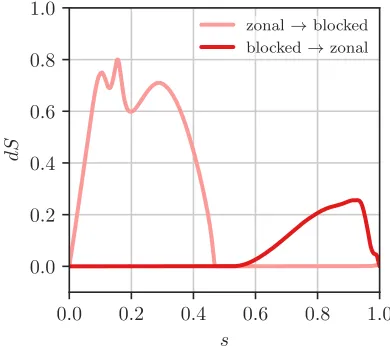
FIG. 2. Action density along the transition trajectories be-tween the zonal and the blocked configuration, wheresis the arclength parameter along the transition. As clearly visible, the transition towards the blocked state occurs at higher ac-tion, making the blocked state relatively more stable.
C. Instantons for stochastic partial differential equations
Many systems of interest in physical applications have continuous spatial variables, i.e. do not fit the framework
of equation (1). Instead, they are stochasticpartial dif-ferential equations (SPDEs). Applying the algorithm of section II A to stochastic processes in infinite-dimensional spaces is nevertheless largely done in practice. The math-ematical foundation is less clear in this case, though, and a few comments are in order.
A stochastic partial differential equation, even in the simplest case of additive Gaussian noise, is possibly ill-posed. Consider for example
∂tU =B(U) +√ε η(x, t), (38)
where U : [0, T]×Rd → Rm and η denotes temporal white noise. If the noise is also not smooth in space, for example if it is white-in-space as well,Eη(x, t)η(x0, t0) =
δ(t−t0)δ(x
−x; ), it is a non-trivial undertaking to make sense of possible non-linear terms in the drift, B(U), especially if the spatial dimension is higher than one. Recent mathematical breakthroughs18specify a rigorous renormalization procedure in specific cases. In regards to LDT, the main concern is whether this renormalization procedure subsists in the limitε→0. For example, in19, it was discussed for the stochastic Allen-Cahn equation (e.g.B(U) =U−U3+κ∂2
xU) in 2 or 3 spatial dimensions,
[image:8.612.78.273.399.572.2]assumed one,
ST(φ) = (RT
0 k∂tφ−B(φ)k2L2dt , if the integral converges,
∞ otherwise,
(39) wherek · kL2 denotes theL2-norm in the spatial
compo-nents. In the following, we will consider SPDE examples, but no longer dwell upon the mathematical intricacies, instead assuming that (39) is valid.
If the rate function takes the form (39), all arguments put forward in the finite dimensional case can be trans-ferred to the SPDE situation, and a corresponding al-gorithm can be constructed. In particular, a gradient descent of the form introduced in section II is still fea-sible, with gradients of vectors replaced by functional derivatives of the corresponding operators. Therefore, equation (31) to compute the descent direction for the SPDE (38) becomes
dk =θk0+ (DφB(φ))>θk, (40)
whereA> is theL2-adjoint of the (differential) operator
Aand Dφ the functional derivative. Consider for exam-ple Burgers equation with periodic boundary conditions, where
B(U) =ν∂2
xU−U ∂xU . (41)
ThenDφB(φ) is the operator
DφB(φ) =ν∂x2−(∂xU)−U ∂x (42)
such that
(DφB(φ))>=ν∂x2+U ∂x. (43)
Recall that we can still computeθ∗, i.e. the minimizer of the inner constrained optimization problem (27) via
θ∗(φ) =µ−1φ0−B(φ) =µ−1φ0−ν∂x2φ+φ∂xφ , (44)
where the last equality holds for the Burgers example with spatio-temporal white noise.
In practice, equation (40) has to be rewritten in order to be practical for the SPDE case, because the involved high spatial derivatives come with Courant-Friedrichs-Levy (CFL20) stability conditions that limit the time-step of the descent, and therefore the convergence rate of the scheme. A detailed discussion of tricks and opti-mizations for the SPDE case is given in16.
D. Example: The stochastic Burgers-Huxley equation
As example for a nonlinear SPDE, we consider the stochastic Burgers-Huxley model,
∂tu+αu∂xu−κ∂x2u=f(u) +
√
εη(x, t), x∈[0,1], (45)
where α > 0 determines the strength of the nonlinear advection term, κ > 0 is the diffusion constant, and
0.0 0.2 0.4 0.6 0.8 1.0
s
0.0 0.2 0.4 0.6 0.8 1.0
[image:9.612.325.561.55.199.2]x
FIG. 3. Maximum likelihood transition pathway of the bi-stable Burgers-Huxley model, transitioning fromu =−1 to u = 1. The transition happens as Allen-Cahn like nucle-ation, but the critical nucleus forms as steepening, asymmet-ric shock-wave. The saddle-point, denoting the critical nu-cleus of the transition, is marked by a dashed line.
the boundary conditions are periodic. The field η(x, t) is spatio-temporal white noise. Forf(u) = 0, this equa-tion is the stochastic Burgers equaequa-tion, arising in com-pressible gas dynamics, traffic flows, and as test-bed for turbulence. With the inclusion of a double-well reaction termf(u) = u−u3, the equation becomes metastable, with two spatially homogeneous stable fixed points at
u=−1 andu= 1. The spatially homogeneous solution
u= 0 is a fixed point as well, but depending on the size ofκmight not be a saddle point with a single unstable direction. Instead, for small enoughκ, we expect Allen-Cahn like nucleation dynamics, but the nucleation must happen as a Burgers-like steepening shock wave. Indeed, as figure 3 shows, this intuition is confirmed by the nu-merics: The creation of the nucleus happens in a spatially asymmetric way, and the nucleating seed travels in space. The spatial resolution for the numerical computation is
Nx= 256, while the temporal resolution isNs= 100.
III. RARE EVENT ALGORITHMS FOR EXPECTATIONS AND EXTREME EVENTS
In this section, instead, we will concentrate on situa-tions where it is indeed feasible to solve the minimization problem by integrating the coupled pair of equations of motion, or instanton equations, to obtain the large de-viation minimizer. As we will see, if applicable, this ap-proach comes with a couple of advantages of both the-oretical and numerical nature. In this section we will therefore first review the class of algorithms based on solving Hamilton’s equations in section III A, that can be used to compute instantons for expectations domi-nated by extreme events. Examples are shown in sec-tion III B applying this algorithm to a system with multi-plicative Gaussian noise, and furthermore in section III C demonstrating the use in an infinite dimensional system, with the additional complication of degenerate forcing (i.e. non-invertible noise covariance matrix). We discuss connections to other fields in section III D and numer-ical details in section III E. A geometric variant of the numerical scheme is introduced in section III F, and im-plemented for an example case in section III G.
A. Instantons for expectations and extreme events
For the stochastic processXε
t of equation (1),
dXtε=b(Xtε)dt+
√
εσ dWt,
consider the random variableF(Xε
T), whereF :Rd →R.
This random variable, also termed the “observable”, acts only on the final configuration of the process. We are in-terested in estimating the tail scaling of its probability density, i.e. in quantifying the likelihood of extreme val-ues of the observable. For example, assume that Xε
t is
a stochastic model describing the interaction of predator and prey in a habitat (cf. section III B). We set out to find the probability of observing an abundance of prey. We might additionally be interested in the most likely amount of predators at this unusual configuration, and the historic development into this event. Or we have a stochastic description of waves (cf. section III C), and are interested in the probability of observing high amplitude waves. Additionally we might ask for the most likely shape of the wave at the moment of extreme elevation, or possibly identify the evolution into the extreme wave event to analyze it for possible mechanisms leading to the amplification.
From the discussion in section I we understand that in the limit ε → 0, the probability of observing the event
F(Xε
T) =z, subject toX0ε=x, fulfills
P(z)exp(−ε−1 inf
φ∈Cz
ST(φ)), (46)
where Cz = {φ∈ AC([0, T],Rd) | φ(0) = x, F(φ(T)) = z}, i.e. the set of continuous trajectories starting and x
that observe the event. Let
I(z) = inf
φ∈Cz
ST(φ), (47)
and define
I∗(λ) = inf
φ∈C(ST(φ)−λF(φ(T))), (48)
withC ={φ∈AC([0, T],Rd)| φ(0) =x}. Here, mini-mization is not constrained at the final point, i.e.C de-scribes the set of continuous trajectories starting at x
regardless of their final point. We can then rewrite
I∗(λ) = inf
φ∈C(ST(φ)−λF(φ(T)))
= inf
z∈Rφinf∈Cz
(ST(φ)−λF(φ(T)))
= inf
z∈R( infφ∈Cz
ST(φ)−λz)
= inf
z∈R(I(z)−λz).
so thatI∗(λ) is the Fenchel-Legendre transform ofI(z). This connection allows us to solve the minimization prob-lem (48) instead of the original probprob-lem (47). The same form can be obtained by considering λ as a Lagrange multiplier to enforce the constraint on the final point.
In terms of Hamilton’s principle, the variations of the argument of the infimum in equation (48) with respect to
φgets one additional term that only applies at the final point, so that the Hamilton’s equations become
( ˙
φ=∇θH(φ, θ) φ(0) =x
˙
θ=−∇φH(φ, θ) θ(T) =−λ∇F(φ(T)). (49)
The difference with Hamilton’s equations of the problem discussed in section II
( ˙
φ=∇θH(φ, θ) φ(0) =x, F(φ(T)) =z
˙
θ=−∇φH(φ, θ) (no boundary conditions) (50)
appears minuscule, but is profound: The φ-equation in (50) has to be solved with initialand final condition, and therefore necessitates shooting methods which are inefficient in high dimension (hence the alternative ap-proach we took in section II). For (49), on the other hand, the equations for bothφandθhave exactly one boundary condition each. It is natural to integrate theφ-equation forward in time, starting at x, while integrating the θ -equation backward in time, starting at −λ∇F(φ(T)). This direction of integration is the only sensible one in the first place: Due to the conjugate momentum equation containing the term−(∇b(φ))>, a numerical integration forward in time would be numerically unstable or even ill-posed. An algorithm to find the instanton in this case then consists of the following steps: Starting from the
k-th guessφk(t) for the instanton trajectory,
(i) solve the equation
˙
θ=−∇φH(φk, θ), θ(T) =−λF(φk(T)) (51)
(ii) solve the equation
˙
φ=∇θ(φ, θ), φ(0) =x (52)
forward in time to obtain the next guessφk+1,
(iii) iterate until convergence.
The convergence properties, stability and possible im-provements of this algorithm are discussed in sec-tion III D. Considering the dual problem (48) instead of the original one (47) comes at a price: Instead of choos-ing directly the valuezof the observable, instead we pre-scribe its dual λ, and obtain the corresponding value of
za posteriori. In other words, we loose the capability of computing the instanton for a specific observable z. In practice, this is usually not a problem, even though the mapz(λ) is not available in general: Typically one is in-terested in the complete distribution ofP(z), and there-fore producing instantons for a whole range ofλsimilarly covers a whole range ofz. Alternatively, a self-correcting version of the algorithm is easily implemented, where λ
is adjusted on-the-fly to achieve the desired outcomez. Note thatI∗(λ) is nothing but the limit of the scaled cumulant generating function of the random variable
F(Xε T), i.e.
I∗(λ) = lim
ε→0εlogEexp(ε
−1λF(Xε
T)). (53)
In this interpretation, we could call the instanton solv-ing (49) also the instanton correspondsolv-ing to the expec-tation
Eexp(ε−1λF(XTε)) (54)
in the limit ε → 0. It is similarly possible to define observables not only on the final point of the trajectory, but for example of the form
F({Xtε}) = Z T
0
f(Xtε)dt or F({Xtε}) = Z T
0h
g(Xtε), dWi
(55) and perform similar arguments, leading to additional drift terms in the conjugate momentum equation.
Finally, while the above arguments rigorously hold un-der suitable conditions in the limitε→0, it is common to loosen conditions on the stochastic process and consider the case ε fixed, but λ → ∞. The intuition is that for largeλonly extreme events of the process are considered, and a large deviation principle might hold for the observ-able even for finite noise. One can then write down ana priori large deviation principle for the random variable
F(Xε
T) and compute the instanton for large values ofλto
probe the tail of the probability to observe the event. It is in this sense that this approach can be considered as in-stantons forextreme events. They are commonly used in practice, for example in fluid dynamics, where an equiv-alent algorithm has been introduced by Chernykh and Stepanov21, which was applied to compute instantons for the Burgers22,23, Navier-Stokes24, and KPZ equations25 as well as the integrated current of the periodic diffusion equation26,27.
0.0 0.1 0.2 0.3 0.4 0.1
0.2 0.3 0.4
0.5 T=10
0.0 0.1 0.2 0.3 0.4 0.1
0.2 0.3 0.4
[image:11.612.319.560.54.352.2]0.5 T=1
FIG. 4. Occurrence of extreme concentration of prey in the Lotka-Volterra model. The streamlines are showing the de-terministic flow field. The heat-map shows the logarithm of a histogram of all trajectories starting at the fixed point that reacha(T) = 0.35 (regardless of b(T)). The white line de-picts the instanton for the expectationEexp(−λa(T)). Even for finiteε, the sample trajectories clearly cluster around the instanton. Shown are two different event times,T = 10 (top) andT = 1 (bottom).
B. Example: Extreme concentration of prey in the Lotka-Volterra model
The Lotka-Volterra system, or predator-prey system, is frequently used in biology as the simplest description of the interaction of two species, one of which preys on the other. In its typical form, it is considered without any fluctuations, but as it can be understood as continuous limit of a network of reactions, it is clear how a noise term can be derived as chemical Langevin equation.
the stoichiometric reaction network
A−→α A+A (reproduction of prey) (56a)
A+B−→β B+B (predation) (56b)
B−→ ∅γ (death of predator) (56c)
∅−→δ A (migration of prey) (56d)
∅−→δ B (migration of predator) . (56e)
Each of these is to be understood as a Poisson process with ratesαtoδ. The first three are standard in Lotka-Volterra, the last two are added to model migration of both species from neighboring habitats towards the con-sidered location. This prevents degeneracy of the forcing at extinct population levels and the difficulty of absorb-ing boundary conditions.
Under the assumption that the typical populationsN
are sufficiently large, ε = N−1 → 0, one can obtain a limiting behavior of the mean concentrations, and supple-ment it with Gaussian noise consistent with the central limit theorem around this mean. The resulting model, often termed chemical Langevin equation28, that corre-sponds to the reaction network (56), then is
(
da= (−βab+αa+δ)dt+√ε√βab+αa+δ dWa, db= (βab−γb+δ)dt+√ε√βab+γb+δ dWb,
(57) wherea, bare functions from [0, T] intoR+, denoting the concentration of predator and prey in the habitat. The stochastic fluctuations are white-in-time Gaussian and zero mean, but notably multiplicative. Note that while this noise term chosen to be consistent with a central limit theorem for N → ∞, it is actually not true that this approximation is valid for large deviations as well. In general, the LDP is sensitive to the non-Gaussian na-ture of the stochastic process defined in (56), which has Poisson statistics. We explain how to treat such non-Gaussian systems correctly in section IV, while here, for simplicity, we are considering the multiplicative Gaussian SDE (57) as given.
We choose the interaction rates α, β, γ, and δ in a way that there exists a unique fixed point (¯a,¯b) at which concentrations of predators and prey are in equilibrium. Concretely, we takeα= 1,β= 5,γ= 1,δ= 0.1. Chang-ing these parameters can produce more complicated at-tractors, such as limit cycles, which we will not investi-gate here. Instead, we are interested in the question of how unlikely high concentrations of prey develop on dif-ferent time framesT when the system starts at the fixed point (¯a,¯b). For that reason, we choose F(a, b) =a(T), i.e. condition on high values ofa(T), regardless ofb(T).
Since this is the first time we encounter multiplicative noise, a few comments are in order. For a system of the form
dXtε=b(Xtε)dt+
√
εσ(Xtε)dWt, (58)
witha(x) = (σσ>)(x), the Hamiltonian is
H(φ, θ) =hb(φ), θi+12hθ, a(φ)θi, (59)
so that an additional term enters the equation for the conjugate momentum,
˙
θ=−∇φH(φ, θ) =−(∇b(φ))>θ+hθ,∇φa(φ)θi, (60)
where the last term is to be understood as (hθ,∇φa(φ)θi)i = Pj,kθj∇φiajkθk. Consequently, the instanton equations for the (stochastic) Lotka-Volterra model are
˙
a=−βab+αa+δ+ (βab+αa+δ)θa
˙
b=βab−γb+δ+ (βab+γb+δ)θb
˙
θa =−(α−βb)θa−βbθb+1
2((α+βb)θ 2
a+βbθ2b)
˙
θb =βaθa−(−γ+βa)θb+12(βaθ2
a+ (γ+βa)θb2),
(61) which have to be solved with the boundary conditions (a(0), b(0)) = (¯a,¯b) and (θa(T), θb(T)) =−λ∇F(a, b) = (−λ,0).
Figure 4 shows the result of applying the algorithm of section III A to this system, and comparing to Monte-Carlo sampling. Here, two different transition times are chosen,T = 1 andT = 10. For T = 10, the system has enough time to explore around the fixed point, but it is obvious that the last portion of the excursion, before it hits a(T) = 0.35, clusters around the instanton trajec-tory. In particular, theb-coordinate at whicha = 0.35 is attained seems to be predicted reasonably well. For
T= 1, instead, the transition trajectory needs to follow a different route, and the endpointa= 0.35 will most likely be attained at higher concentration of predators. Some points, such as (a, b) = (0.25,0.3), are almost never vis-ited forT = 10, but are very likely underT = 1, which is correctly predicted by the instanton computation. Note that the heat-map depicting the empiric probability den-sity in figure 4 has a logarithmic color-map for the tails to remain visible. Deviations from the optimal path are therefore very unlikely indeed.
Parameters for T = 1 are ∆t = 10−2, ε = 0.005 and
λ= 0.4209, and for T = 10 are ∆t = 10−2, ε = 0.004, andλ= 0.2106. Roughly 5·106trajectories were sampled for the Monte-Carlo estimate.
C. Example: Extreme amplitudes in the Korteweg-de Vries equation
Consider for the fieldu(x, t) : [0,2π]×[0, T]→Rthe stochastic partial differential equation
∂tu+u∂xu+κ∂x3u−ν∂2xu=η(x, t), u(x, t= 0) = 0,
(62) with periodic boundary conditions in space, and x ∈
−π −π/2 0 π/2 π x
0 5
10 t= 0.0
t= 0.25
t= 0.5
t= 0.75
[image:13.612.58.299.54.201.2]t=T = 1
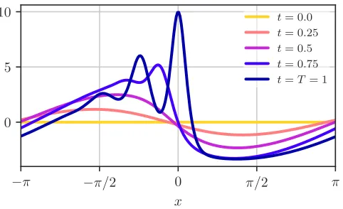
FIG. 5. Evolution of the Korteweg-de Vries instanton into a large amplitude at the final time T = 1, starting from rest and forcing only the largest Fourier mode of the system.
through the forcingη and energy dissipation through a diffusion term with viscosity ν. For the forcing, we de-mand that, in Fourier space,
Eηkˆ (t)ˆηq(t0) =εδ(t−t0) ˆχq−k, (63)
where ˆχ :Z →R is the forcing spectrum and ˆηk is the
k-th mode of the Fourier transform ofη.
Intuitively, for a ˆχk with compact support only for smallk, the forcingη(x, t) inserts energy on large scales, and the nonlinearity transfers those to smaller scales, on which dispersion and dissipation act on them. We are interested how this nonlinear cascading effect produces waves of extreme amplitude. To this effect, we choose an observable
F(u(x, T)) = (φ∆? u)(x, T), (64)
with φ∆(x) = Aexp −x2/∆2
, and ? denoting spatial convolution. For small ∆, this observable selects high amplitudes in close proximity tox= 0, i.e. at the center of the domain, and therefore generates high wave eleva-tions at this position. As forcing spectrum, we want
χk= (
1 if|k|= 1
0 otherwise, (65)
which inserts energy only into the largest mode of the sys-tem. This is the first time we considerdegenerateforcing, in that only a subset of the available degrees of freedom are forced, or, equivalently, the noise covariance matrixa
of (1) is not invertible. This poses practical problems for algorithms based on global minimization discussed in sec-tion II, where heavy use is made of either thea-norm, or
θis expressed asθ=a−1( ˙φ
−b(φ)). For these algorithms, the inverse has to be replaced by the pseudo-inverse (see section 3.4 of1), and the degenerate forcing introduces additional stiff constraints for the unforced modes, as those effectively behave deterministically (and thus are attained with infinite action if they deviate from the de-terministic behavior). For the Hamilton’s equations, and
the algorithm discussed in this section, the noise corre-lation is never inverted, and degenerate forcing can be treated without extra effort.
The instanton equations corresponding to the posed problem are
(
∂tu+u∂xu+κ∂3
xu−ν∂2xu=χ ? θ, u(x, t= 0) = 0, ∂tθ+u∂xθ+κ∂3
xθ+ν∂x2θ= 0, θ(x, t=T) =−λφ∆(x),
(66) where χ(x) is the inverse Fourier transform of the forc-ing spectrum. The instanton computed by solvforc-ing equa-tions (66) is depicted in figure 5. It is clearly visible that a high final amplitude around x = 0 is achieved by a combination of non-linear advection and dispersion. Ad-ditionally, the final configuration clearly contains Fourier modes different from|k| = 1, implying that indeed the non-linearity cascaded energy into higher modes in a way to optimize the final amplitude. Note also that because of ∆1, we are merely demanding a large amplitude at
x= 0, but leave the rest of the wave form unconstrained. The elevation profile in the rest of the domain is chosen in a most likely manner, and the curves shown in figure 5 can be interpreted as the prototypical way of forming the considered amplitude. The model parameters areT = 1, ∆ = 10−1, α=κ= 4·10−2, λ= 1, andA= 0.25. The numerical parameters are Nx = 256, Nt = 1000, and ∆t= 10−3.
D. Connections to optimal control
It is instructive to formulate the optimization prob-lem (46) in the language of optimal control29: We are interested in finding theoptimal control p: [0, T]→Rd such that forX ∈Rd, the system
˙
X(t) =b(X(t)) +p(t), X(0) =x , (67)
has the desired outcome, F(X(T)) = z. We penalize large values ofpby choosing
J(p) =12 Z T
0 |
p(t)|2dt (68)
as cost function. In other words, we are searching for the optimal noise realizationpto drive the system into a final state where F(X(T)) = z. To obtain a mini-mization procedure that honors the constraints given by the observable and equation (67), we introduce Lagrange multipliers ξ ∈ [0, T]×Rd and λ ∈ R, such that we attempt to minimize
E(p) = 1 2
Z T
0 |
p(t)|2dt+λF(X(T))
+ Z T
0 h
Its total variation is given by
δE(p) =hp−ξ, δpi+hX˙−b(X)−p, δξi+hX(0)−X, δξ(0)i
+λh∇F(X(T)), δX(T)i+h−ξ˙−(∇b(X))>ξ, δXi
+hξ(T), δX(T)i − hξ(0), δX(0)i.
We can read of the desired conditions to fulfill the con-straints as
( ˙
X =b(X) +p, X(0) =x
˙
ξ=−(b(X))>ξ, ξ(T) =
−λ∇F(X(T)), (69)
and the gradient of the cost functionalE(p) with respect to the controlpis then given as
δE(p)
δp =p−ξ . (70)
We immediately identify that the conjugate momentum
θ is the variable ξ in optimal control, often termed the adjoint variable. Second we realize that the forward and adjoint equations are identical to the instanton equations. Therefore, the iterative algorithm given in section III A is nothing but a gradient descent for the cost functional
E(p), with step length 1. This not only answer questions about (local) convergence of the algorithm of section II A, but furthermore allows to improve stability and order of convergence of the algorithm. First, it is almost always necessary to adjust the step size for each iteration ac-cording to a line search strategy to achieve convergence. Second, one might consider pre-conditioning, to allow for faster convergence. Lastly, the computation of the descent direction −δE/δp from equation (70) allows to construct higher order optimization algorithms, such as nonlinear conjugate gradient or quasi-Newton methods.
Note that, similar to the argument above, for practical reasons we choose to not consider variations with respect to λ, and instead consider λ ∈ R given a priori to es-tablish a mapping λ(z) from z(λ) = F(X∗(T)), where
X∗(T) depends on λthrough the boundary condition of the adjoint equation (69).
E. Improvements and implementation considerations
A few remarks are in order to point out possible im-provements and implementation concerns when solving Hamilton’s equations.
• While solving a global minimization problem as in-troduced in section II necessitates a complicated procedure to compute descent directions, the so-lution of Hamilton’s equations put forward in this section usually comes at a much lower implemen-tation cost: Given a stochastic problem at hand, one likely has already available an efficient solver of the forward equation, just replacing stochastic noise with a function of the conjugate momentum. The backward equation (auxiliary equation, adjoint
equation), on the other hand, is often available as well for professional software packages, usually from automatic differentiation, in order to quan-tify the uncertainty from the adjoint field ξ. In this case, a computation of the instanton might be achieved in a truly “black-box” form, where the it-erative solution of the Hamilton’s equations can be achieved without modifying the original software.
• The mutual dependency of the forward and back-ward equations necessitates in principle that the whole trajectory is stored in its entirety. While this is usually feasible for finite-dimensional problems, it quickly becomes prohibitive in terms of memory requirement when talking about SPDEs in many di-mensions, where usually the storage requirements are chosen to be of the order of magnitude of a single state of the field variables, and not a contin-uous trajectory. In optimal control, this restriction is usually overcome viacheckpointing mechanisms, where one does not save to memory a complete tra-jectory, but instead only retains checkpoints, from which subsequent states can be deduced. In its most efficient form, this checkpointing can be im-plemented in a recursive manner, leading generally to memory requirements ofO(logNt) instead of the naiveO(Nt), whereNtis the number of discretiza-tion points in time. Some details of the applicadiscretiza-tion of this method to instanton computations is laid out in30.
• The nature of the conjugate momentum as adjoint variable, as discussed in section III D, highlights its adjointness to the main field variable. Would one discretize the action, and consider forward and backward equation as their discrete variation, this state of affairs would necessitate the usage of a spe-cial temporal integration scheme for the numerical solution of the adjoint equation, namely a tempo-ral integration scheme that is adjoint to the for-ward scheme. Some time integration schemes (such as the forward Euler scheme) have the property of being self-adjoint, and thus can be used for both equations. The failure to use a correct pair of in-tegration schemes generally results in the failure to converge to the minimum of the cost function.
A more detailed discussion of implementation concerns of this technique in the infinite-dimensional case, specif-ically with the application to fluid mechanics, is given in24,30.
F. Geometric version of the Hamilton’s equations
−20 −10 0 10 20
x −1.0
−0.5 0.0 0.5 1.0 1.5
u
(
x,
t
=
0)
geometric
T= 1000
T= 100
T= 10
−20 −10 −0.05
0.00
[image:15.612.55.300.54.211.2]0.05
FIG. 6. Comparison of the final condition of the instan-ton, u(x, t = 0), conditioning on extreme gradients in the origin, for the geometric parametrization and physical time parametrizations for varyingT. As visible in the inset, only forT = 1000, secondary extrema disappear.
this is needed to calculate expectations with respect to the invariant measure of the process, assuming it exists. For algorithms based on the minimum action method (MAM)14, the additional complication the minimization over T > 0 introduces is resolved by invoking Mauper-tuis principle and focusing on the computation of the geometric minimizer, i.e. realizing that the minimizing trajectory can be computed without explicit reference to its parametrization.
For algorithms based on the Hamilton’s equation, sim-ilar ideas and extensions exists31: Instead of solving the original Hamilton’s equations (16), we can choose a reparametrizations(t), and consider Hamilton’s equa-tions in this parameter,
(
φ0 =µ∇θH(φ, θ)
θ0=µ
∇φH(φ, θ), (71)
where the prime denotes derivatives with respect to s
and µ = dt/ds. Now, as pointed out in section II A, µ
can be interpreted as Lagrange multiplier enforcing the Hamiltonian constraint, and is available as
µ= kφ 0
k2 ∼
hφ0,∇θHi ∼
= kφ 0
ka
kb(φ)ka
, (72)
where the much simpler second form only holds for Gaus-sian additive noise of the form (1) (compare section II A).
G. Example: Extreme gradients of the stochastic Burgers equation
As an example, following31, consider for the field
u(x, t) : [−L/2, L/2] ×[−T,0] → R the stochastic Burger’s equation,
∂tu+u∂xu−ν∂2xu=η(x, t), u(x, t=−T) = 0, (73)
with periodic boundary conditions in space. Here, we consider a noise termη that is white in time, but has a finite correlation length in space,
Eη(x, t)η(x0, t0) =εδ(t−t0)χ(x−x0), (74)
and we prescribe the specific correlation in Fourier space of
ˆ
χ(k) =k2exp(
−k2/2)
H(kc− |k|),
whereH denotes the Heaviside step function. In effect, the forcing correlation has the shape of a “Mexican hat” function, with cut-off wave numberkc. Effectively, equa-tion (73) can be considered as a test-bed for turbulence, where energy is inserted on large scales due to the forcing, and then cascades to smaller scales via the nonlinearity, where it dissipates. We focus on events that lead to a strong negative gradient at the final time, t = 0, and therefore choose an observable
F(u(x,0)) = (φ∆? ∂xu)(x,0), (75)
where, identically to the KdV-case in (64),φ∆ mollifies on scales ∆, so that here we concentrate on high gradients at the origin.
In order to probe for events on the invariant mea-sure of (73), we want to consider the limit T → ∞, and therefore need to either consider extremely large time intervals T, or alternatively employ the geomet-ric variant of the Hamiltonian formalism as proposed in (71), where the norm is induced by the covarianceχ(x), i.e. kvk =hv, χ−1(x)vi1/2 on its support. For technical details, see31. Given this setup, figure 6 compares the fi-nal condition of the instanton between finite timesT and the limitT → ∞ obtained in the geometric formalism. It demonstrates how, for choices T = 10 or T = 100, unphysical secondary maxima are present (compare in-set of figure 6), that disappear in the infinite time case, and withT = 1000. Similarly, one can look at the value of the HamiltonianH(u, p), which necessarily disappears for large T, limT→∞H = 0, and consider the quantity max(|H|) along the instanton trajectory as measure of the numerical error of the discretization. In this metric, the geometric variant for the same number of discretiza-tion points in time, is roughly 104 times more accurate than the naive parametrization with physical time31.
IV. GENERALIZATIONS TO THE NON-GAUSSIAN CASE
above form, as can be guessed from the fact that both MAM-style global minimization of section II and the al-gorithms based on the solution of Hamilton’s equations of section III are written in terms of a generic large devia-tion Hamiltonian. In this secdevia-tion, we therefore intend to broaden the scope by demonstrating how more generic large deviation Hamiltonians are obtained, and corre-sponding instantons can be computed with the above algorithms. In particular, the Gaussianity of the un-derlying stochastic process is reflected in the fact that the Hamiltonian is quadratic in its conjugate momen-tum. Other processes, most notably those that result from limits of continuous time Markov jump processes (MJPs), generally lead to a non-quadratic Hamiltonian.
A. Large deviation principles as WKB approximation
Consider a homogeneous continuous time Markov jump process Xt, t ∈ [0, T], with state space E. The process is completely characterized by its generator L, which allows us to write down its backward Kolmogorov equation (BKE) as
∂tf+Lf = 0, f(T) =φ (76) for
f(T−t, n) =Enφ(Xt), (77) where n ∈ E, f : [0, T]× E → R, and φ: E → R. For concreteness, consider as a state space a counting space
E =ZN+ forN ∈N different species, where individuals of each species can interact viaR∈Nindependent Pois-son processes, manipulating the number of individuals of each species. For each of theRdifferent interactions, the number of individuals changes from n to n+νr, where
νr ∈ZN, with a rate ˜ar(n), r ∈ {1, . . . , R}. Then, the
corresponding generator reads
(Lf)(n) =
R X
r=1 ˜
ar(n) (f(n+νr)−f(n)). (78)
Rescaling this into new variablesx=n/M, whereM is a typical number of individuals, we can expand inε=M−1 to obtain a large deviation principle in the limit of many individuals. To this end, consider the generator in the rescaled variables,
(Lεf)(x) = R X
r=1
ar(x) (f(x+ενr)−f(x)), (79)
where ar is defined on the rescaled variables. We now evaluate this rescaled generator onto a function of the form exp(ε−1g(x)) and rescale time withεappropriately. This corresponds to a WKB approximation of the BKE, or equivalently to the method of Feng and Kurtz34 (com-pare also35), and yields
∂tg(x) +
R X
r=1
ar(x)eε−1(g(x+ενr)−g(x))
= 0, (80)
0 25 50 75 100 125 150
a
0 1 2 3
b
[image:16.612.320.561.55.201.2]relaxation dynamics instanton
FIG. 7. Instanton for the non-Gaussian genetic switch. The arrows denote the direction of the deterministic flow, the red solid line depicts the minimizer, the red dashed line the relax-ation path from the saddle. Red dots are located at the fixed points (stable and unstable). The whole figure is a zoom into the uphill region, the other stable fixed point is far up the upper left corner.
which can be expanded, to leading order inε, into
∂tg(x) +
R X
r=1
ar(x)ehνr,∇g(x)i−1= 0. (81)
Equation (81) can be interpreted as Hamilton-Jacobi equation
∂tg(x) +H(x,∇g(x)) = 0, (82)
with
H(x, θ) =
R X
r=1
ar(x)ehνr,θi−1. (83)
The Hamiltonian (83) is precisely the large deviation Hamiltonian in that the large deviation rate function is the time integral of its Fenchel-Legendre transform. The Hamiltonian (83) is furthermore a prime example of a non-quadratic Hamiltonian.
Note that applying the same method to the generator of the SDE (1),
(Lεf)(x) =hb(x),∇if(x) +ε
2
d X
i,j=1
aij∇i∇jf(x) (84)
recovers exactly the expected Hamiltonian (17) for the leading order inε.
B. Example: Genetic switch
want to consider a simplified model of a genetic switch based on a model discussed in36: Inside a bacterium, plasmids contain genes that encode two different pro-teins, A and B. Each protein is able to form polymers that inhibit the production of the other protein, respec-tively. In the emerging situation, the cell may exist in a state close to one of two fixed points: Either protein
A dominates, and inhibits the production of proteinB, while the production of A remains high. Alternatively, proteinB dominates, and inhibits the production of A. Rarely, fluctuations may arise that push the system from one fixed point to the other.
We choose to model this system by describing the con-centrations of proteinsA andB bya∈R+ andb∈R+, respectively. There are four reactions in total, namely production and degradation of A and B, leading to the reaction network
∅ pA(b)
−−−→A (production ofA) (85a)
∅ pB(a)
−−−−→B (production ofB) (85b)
A−−−−→ ∅dA(a) (degradation ofA) (85c)
B dB(b)
−−−→ ∅ (degradation ofB) (85d)
with rates
pA(b) =C/(1 +b3), pB(a) =D/(1 +a),
dA(a) =a, dB(b) =b . (86)
The corresponding large deviation Hamiltonian, using equation (81), is thus
H(a, b, θa, θb) = C 1 +b3(e
θa−1) +a(e−θa−1)
+ D
1 +a(e
θb−1) +b(e−θb−1). (87)
The minimizer for this setup, as well as the relaxation paths from the saddle, are depicted in figure 7. They are computed by implementing the algorithm presented in section II A for the Hamiltonian (87) for the transition between the two fixed points. The model parameters here are chosen to beC= 156 and D= 30.
V. SYSTEMS WITH RANDOM PARAMETERS AND EXTREME EVENTS
Up to now, all discussions in the previous sections con-cerned sample path large deviations, where a stochastic process realizes a rare event almost surely by following a trajectory that minimizes the corresponding action func-tional. In this section, we are focusing on a related, but different setup of a dynamical system with random pa-rameters. Given a distribution of the random parame-ters, we want to reason about probabilities to observe certain events, and again characterize the rare ones by
dominating configurations of parameters. To this effect, consider foru: [0, T]→Rd the dynamical system
∂tu=b(u, θ), u(t= 0) =u0(θ), (88)
whereθ∈Ω⊆RM is the set of M random real param-eters, distributed according to a measure µ. Since the initial conditions and the drift of equation (88) depend on the random parameters, the solution is a random vari-able, denoted byu(·, θ). We can then try to quantify the probability of an observable exceeding a thresholdz∈R, for example at the final time, or integrated over time, or as temporal maximum, i.e.
PT(z) =P(F(θ)≥z), F(θ) =
f(u(T, θ)) or RT
0 f(u(t, θ))dt or max
0≤t≤Tf(u(t, θ)).
(89)
A. Large deviations for systems with random parameters
Indeed, if in the limit of large z this probability be-comes small, limz→∞PT(z) = 0, then under some ad-ditional assumptions on F : Ω → R we have a large deviation principle as a contraction principle of the form
PT(z)exp(− min
θ∈Ω(z)I(θ)), (90)
in the limitz→ ∞, where the set Ω(z)⊆Ω is the set of permissible random parameters,
Ω(z) ={θ∈Ω|F(θ)≥z}, (91)
and the rate function I(θ) is obtained as the Legendre transform of the cumulant generating function ofθ,
I(θ) = max
η (hη, θi −S(η)), (92)
for
S(η) = logEexphη, θi= log Z
Ω
exphη, θidµ(θ). (93)
The minimizer ofI(θ) in Ω(z), i.e.
θ∗(z) = argmin
θ∈Ω(z)
I(θ), (94)