An improved closed loop stability related measure for finite precision digital controller realizations

[6] H. Ito, “Overlapping decomposition for multirate decentralized control,” in Preprints 8th IFAC/IFORS/IMACS/IFIP Symp. Large Scale Systems: Theory and Applications, vol. 1, Patras, Greece, 1980, pp. 259–264. [7] K. Malinowski and M. Singh, “Controllability and observability of

ex-panded systems with overlapping decompositions,” Automatica, vol. 21, pp. 203–208, 1985.

[8] J. M. Rossell, “Contribution to decentralized control of large-scale sys-tems via overlapping models,” Ph.D. dissertation (in Spanish), Tech. Univ. Catalunya, Barcelona, Spain, 1998.

[9] D. D. ˇSiljak, Decentralized Control of Complex Systems. New York: Academic, 1991.

[10] D. D. ˇSiljak, S. M. Mladenovic´, and S. Stankovic´, “Overlapping decen-tralized observation and control of a platoon of vehicles,” in Proc. Amer. Control Conf., San Diego, CA, 1999, pp. 4522–4526.

[11] E. D. Sontag, Mathematical Control Theory. New York: Springer-Verlag, 1990.

[12] S. S. Stankovic´, S. Mladenovíˇc, and D. D. ˇSiljak, “Headway control of a platoon of vehicles based on the inclusion principle,” in Complex Dynamic Systems with Incomplete Information. Aachen, Germany: Shaker Verlag, 1998, pp. 153–167.

[13] S. S. Stankovic´, X. B. Chen, and D. D. ˇSiljak, “Stochastic inclusion prin-ciple applied to decentralized control automatic generation control,” Int. J. Control, vol. 72, no. 3, pp. 276–288, 1999.

[14] S. S. Stankovic´ and D. D. ˇSiljak, “Contractibility of overlapping decen-tralized control,” in Proc. Amer. Control Conf., Chicago, IL, 2000, pp. 811–818.

An Improved Closed-Loop Stability Related Measure for Finite-Precision Digital Controller Realizations

J. Wu, S. Chen, G. Li, R. H. Istepanian, and J. Chu

Abstract—The pole-sensitivity approach is employed to investigate the stability issue of the discrete-time control system, where a digital controller, implemented with finite word length (FWL), is used. A new stability related measure is derived, which is more accurate in estimating the closed-loop stability robustness of an FWL implemented controller than some existing measures for the pole-sensitivity analysis. This improved stability measure thus provides a better criterion to find the optimal realizations for a generic controller structure that includes output-feedback and observer-based con-trollers. A numerical example is used to verify the theoretical analysis and to illustrate the design procedure.

Index Terms—Closed-loop stability, digital controller, finite word length, optimization.

I. INTRODUCTION

The current controller design methodology often assumes that the controller is implemented exactly, even though in reality a control law

Manuscript received May 15, 2000; revised October 5, 2000 and January 30, 2001. Recommended by Associate Editor T. Chen. The work of the first two authors was supported by the UK Royal Society under a KC Wong fellowship (RL/ART/CN/XFI/KCW/11949).

J. Wu and J. Chu are with the National Laboratory of Industrial Control Tech-nology, Zhejiang University, Hangzhou, 310027, P. R. China.

S. Chen is with the Department of Electronics and Computer Sci-ence, University of Southampton, Southampton SO17 1BJ, U.K. (e-mail: [email protected]).

G. Li is with the School of Electrical and Electronic Engineering, Nanyang Technological University, Singapore.

R. H. Istepanian is with the Department of Electronic and Computer Engi-neering, Brunel University, Uxbridge, Middlesex UB8 3PH, UK.

[image:1.612.324.532.62.203.2]

Publisher Item Identifier S 0018-9286(01)06599-0.

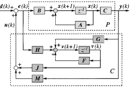
Fig. 1. Discrete-time closed-loop system with a generic digital controller.

can only be realized in finite precision. It is well-known that a designed stable control system may achieve a lower than predicted performance or even become unstable when the controller is implemented with a finite-precision device. It has been noted that a controller design can be implemented with different realizations and that the FWL effect on the closed-loop stability depends on the controller realization structure. This property can be utilized to select controller realization in order to improve the robustness of closed-loop stability under controller pertur-bations. Currently, two approaches exist for determining the optimal controller realizations under different criteria, namely pole-sensitivity measures [1]–[5] and complex stability radius measures [6], [7].

In the first approach, the pole sensitivity measures based on a 2-norm [2] and a 1-norm [3] are used to quantify the FWL effect, leading to a nonconvex and nonsmooth optimization problem in finding an optimal FWL controller realization. Efficient global optimization techniques to solve for this optimization problem are readily available [4], [5], [8]. Fialho and Georgiou [7] used the complex stability radius measure to formulate an optimal FWL controller realization problem that can be represented as a specialH1norm minimization problem and solved for with the method of linear matrix inequality [9], [10]. In this second approach, the FWL perturbations are assumed to be complex-valued. Although this assumption is somewhat artificial, the approach has cer-tain attractive features and requires further investigation.

The contribution of this note is twofold. First, a generic con-troller structure is considered that includes output-feedback and observer-based controllers. Second, adopting the pole-sensitivity approach, a new stability related measure is proposed for the unified controller structure and an optimization procedure is developed to find the optimal controller realization that maximizes this new measure. Through theoretical analysis and numerical results, it is shown that this improved measure is less conservative in estimating the FWL closed-loop stability robustness of a controller realization than the existing pole-sensitivity measures of [2], [3].

II. PROBLEMFORMULATION

Consider the discrete-time closed-loop control system depicted in Fig. 1, where the linear time-invariant plantP is described by

x(k + 1) = Ax(k) + Be(k)

y(k) = Cx(k) (1)

which is completely state controllable and observable with

A 2 Rn2n_{,B 2 R}n2p _{and C 2 R}q2n_{; and the digital}

con-trollerC is described by

v(k + 1) = Fv(k) + Gy(k) + He(k)

u(k) = Jv(k) + My(k) (2)

with F 2 Rm2m,G 2 Rm2q, J 2 Rp2m, M 2 Rp2q and

H 2 Rm2p_{. The output-feedback and observer-based controllers can}

be unified in this general structure:C is an output-feedback controller whenH = 0; a full-order observer-based controller when F = A 0

GC, M = 0 and H = B; a reduced-order observer-based controller,

otherwise [11], [12].

Assume that a realization(F0; G0; J0; M0; H0) of C has been

designed. It is well-known that the realizations ofC are not unique. All the realizations ofC form the realization set

S= (F; G; J; M; H): F = T1 01_F

0T; G = T01G0;

J = J0T; M = M0; H = T01H0 (3)

whereT 2 Rm2m is any real-valued nonsingular matrix, called a similarity transformation. Letw_F = Vec(F), where Vec(1) denotes the column stacking operator. The vectorswF ,wG,wG ,wJ,wJ ,

wM,wM ,wHandwH are similarly defined. Denote

w = w1

.. .

wN 1

= wF

wG

wJ

wM

wH

and w01=

wF

wG

wJ

wM

wH

(4)

whereN = (m + p)(m+ q)+ mp. We also refer to w as a realization ofC. The stability of the closed-loop system in Fig. 1 depends on the eigenvalues of the matrix

A(w) = _{GC + HMC F + HJ}A + BMC BJ

= _{0 T}I 001 A(w0) _{0 T}I 0 : (5)

All the different realizationsw have the same set of closed-loop poles if they are implemented with infinite precision. Since the closed-loop system is designed to be stable, the eigenvalues

i A(w)

= i A(w0) < 1; 8 i 2 f1; . . . ; m + ng: (6) When aw is implemented with a fixed-point processor, it is per-turbed intow + 1w due to the FWL effect. Each element of 1w is bounded by6=2,

k1wkmax=1 max

i2f1; ...; Ngj1wij =2: (7)

The value of is determined as follows. For a fixed point processor ofBsbits, letBs = Bi+ Bf, where2B is the smallest normaliza-tion factor that makes the absolute value of each element of20B w no larger than 1. Thus,B_iare bits needed for the integer part of a number andBf are bits for implementing the fractional part of a number. It is easy to see

= 20B _{: (8)}

With the perturbation1w, _i(A(w)) is moved to _i(A(w + 1w)). If an eigenvalue of A(w + 1w) is outside the open unit disk, the closed-loop system, designed to be stable, becomes unstable with an FWL implementedw. It is, therefore, critical to know when the FWL error will cause the closed-loop instability. This ultimately means that we would like to know the largest open “sphere” in the controller per-turbation space, within which the closed-loop remains stable. The size or radius of this “sphere” is defined by [6]

0(w)= inf k1wk1 max: A(w + 1w) is unstable : (9) From the definition of0(w), it is obvious that

Proposition 1: A(w + 1w) is stable if k1wkmax< 0(w).

The larger0(w) is, the larger FWL error the closed-loop stability

can tolerate. LetB_sminbe the smallest word length that, when used to

implementw, can guarantee the closed-loop stability. Bmin_s is gener-ally unknown. An estimate ofBmin_s can be obtained by

^ Bmin

s0 = Bi+ Int [0 log2(0(w))] 0 1 (10) where the integerInt[x] x. It can easily be seen that the closed-loop system remains stable ifw is implemented with a fixed-point processor of ^B_s0min. As0(w) is a function of the controller realization w, an

optimal realization can be found that maximizes₀(w). The diffi-culty however is that computing the value of0(w) is an unsolved

open problem. A practical solution is to consider a lower bound of the stability measure0(w) in some sense, which is computationally

tractable. Obviously, the closer such a lower bound is to0(w), the

less conservative the estimation will be. The pole sensitivity measures [2], [3] can be regarded as such lower bounds.

III. A NEWFWL STABILITYRELATEDMEASURE

Roughly speaking, how easily the FWL error 1w can cause a stable control system to become unstable is determined by how close

ji(A(w))j are to 1 and how sensitive they are to the controller

parameter perturbations. We propose the following FWL stability related measure1

1I(w)=1 min i2f1; ...; m+ng

1 0 i A(w)

i(w) (11)

with

i(w)1=

X=F; G; J; M; H

(wX) @ i_@wA(w) X

1

(12)

where, for a vectorx 2 Cs, the 1-normkxk1is defined as

kxk1=1 s

i=1

jxij (13)

and the indicator function(x) is given by

(x) = 0; if x is a zero vector_{1; otherwise.} (14)

Defining a perturbation subset to the controller realizationw

P(w)= 1w: 1 i A(w + 1w) 0 i A(w)

k1wkmaxi(w); 8 i (15)

we have the following proposition, the proof of which is straightfor-ward.

Proposition 2: A(w + 1w) is stable if 1w 2 P(w) and k1wkmax < 1I(w).

Remarks: The requirement for1w 2 P(w) is not too restricted. In practice, we will only be interested in those1w that lie in the bounded region:Q(w)1= f1w: (1w) < 0(w)g, i.e., those 1w that will

not cause the closed-loop instability. Similar to [5] it can be shown that

P(w) exists and at least a large part of Q(w) is covered by P(w).

Define

(P(w)) 1= inf

1w =2P(w)k1wkmax: (16)

Corollary 1: 1I(w) 0(w) if (P(w)) > 0(w).

It can be seen that_1I(w) is a lower bound of ₀(w), provided that

0(w) is small enough. The assumption of small 0(w) is generally

valid, and most of digital control systems do have a small stability ro-bustness, especially when fast sampling is applied. In practice, it is very difficult to verify the sufficient condition(P(w)) > 0(w), as this

would require to know0(w). However, the conditions for Proposition

2 are verifiable.

The stability related measure1I(w) is computationally tractable,

as it can be shown that

@ i A(w)

@F = [ 0 I ]Li(w) 0

I (17)

@ i A(w)

@G = [ 0 I ]Li(w) CT

0 (18)

@ i A(w)

@J = [ BT HT]Li(w) 0

I (19)

@ i A(w)

@M = [ BT HT]Li(w) CT

0 (20)

@ i A(w)

@H = [ 0 I ]Li(w)

CT_MT

JT (21)

withT denoting the transpose operator and

Li(w) = Re 3

i A(w) y3i A(w) xTi A(w)

i A(w)

(22)

wherexi(A(w)) and yi(A(w)) are the right and reciprocal left

eigen-vectors related to thei(A(w)), respectively, 3 denotes the conjugate

operation andRe[1] the real part. Similar to (10), an estimate of B_smin can be provided with1I(w) by

^ Bmin

s1I = Bi+ Int [0 log2(1I(w))] 0 1: (23)

Provided that the conditions of Proposition 2 and Corollary 1 are met,

^ Bmin

s1I ^Bs0min Bsmin. Unlike ^Bmins0 , however, ^Bs1Imincan be

com-puted easily.

An existing stability related measure, which is also computationally tractable, is defined as [3]

1(w)=1 min i2f1; ...; m+ng

1 0 i A(w)

i(w) (24)

with

i(w)=1

X=F; G; J; M; H

(wX) @i_@wA(w) X

1

: (25)

An estimate ofB_sminis provided with1(w) by

^

Bs1min= Bi+ Int [0 log2(1(w))] 0 1: (26) The key difference between1I(w) and 1(w) is that the former

considers the sensitivity ofji(A(w))j while the latter considers the

sensitivity ofi(A(w)). It is well known that the stability of a linear

discrete-time system depends only on the moduli of its eigenvalues. As

1(w) includes the unnecessary eigenvalue arguments in

considera-tion, it is reasonable to believe that1(w) is conservative in

compar-ison with1I(w). This can strictly be verified. Noting

@ i A(w)

@wj

= Re 3

i A(w) @i_@wA(w)

j i A(w) (27)

one has

@ i A(w)

@wj

3

i A(w) @i_@wA(w) j

i A(w) =

@i A(w)

@wj (28)

which means that i(w) i(w). We conclude that 1(w)

1I(w) and ^Bmins1 ^Bs1Imin. Notice that1I(w) is also superior in this

sense than another measure based on a 2-norm [2] called₂(w), since

it has been shown that under the similar conditions2(w) 1(w)

[3].

IV. OPTIMIZATIONPROCEDURE

As different realizationsw yield different values of 1I(w), it is of

practical importance to find awoptthat maximizes1I(w), since the

controller implemented withwoptcan tolerate a maximum FWL error. This optimal realization problem is formally defined as

= max1

w2S1I(w): (29)

Given w0, 8 i 2 f1; . . . ; m + ng, partition xi(A(w0)) and

yi(A(w0))

xi A(w0) = xi; 1 A(w0)

xi; 2 A(w0)

yi A(w0) =

yi; 1 A(w0)

yi; 2 A(w0)

(30)

where xi; 1(A(w0)), yi; 1(A(w0)) 2 Cn and xi; 2(A(w0)),

yi; 2(A(w0)) 2 Cm. It is easily seen from (5) that

xi A(w) = xi; 1 A(w0)

T01_x

i; 2 A(w0)

yi A(w) =

yi; 1 A(w0)

TT_y

i; 2 A(w0)

: (31)

From (17)–(21), we have

@ i A(w)

@F = TTLi; 2; 2(w0)T0T (32) @ i A(w)

@G = TTLi; 2; 1(w0)CT (33)

@ i A(w)

@J = BTLi; 1; 2(w0)+HT0Li; 2; 2(w0) T0T (34) @ i A(w)

@M = BTLi; 1; 1(w0)+HT0Li; 2; 1(w0) C (35)

@ i A(w)

@H = TT Li; 2; 1(w0)CTMT0+Li; 2; 2(w0)JT0 (36)

where

Li; j; l(w0)=Re 3

i A(w0) y3i; j A(w0) xTi; l A(w0)

i A(w0) ;

j; l = 1; 2: (37)

Define the following cost function:

f(T)=1 min

i2f1; ...; m+ng

1 0 i A(w0)

i(w) = 1I(w): (38)

The optimal realization problem (29) can then be posed as the following optimization problem:

=1 max f(T): (39)

Although f(T) is nonsmooth and nonconvex, efficient global op-timization methods exist for solving for this kind of opop-timization problem. The adaptive simulated annealing (ASA) [8] is such an algorithm and is adopted in this study to search for a true global optimumTopt of the problem (39). With Topt, we can obtain the optimal realizationwopt.

V. ANILLUSTRATIVEEXAMPLE

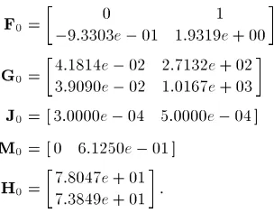
A numerical example is used to illustrate the design procedure and verify the theoretical results given in Section III. The plant model used is a modification of the plant studied in [2] which was a single-input–single-output (SISO) system. We have added one more output that is the first state in the original plant model. The state-space model of this modified plant is given by (40), shown at the bottom of the page. The closed-loop poles as given in [2] were used in design, and the designed reduced-order observer-based controller obtained using a standard design procedure [12] had the form

F0= _{09:3303e 0 01 1:9319e + 00}0 1

G0= 4:1814e 0 02 2:7132e + 02_{3:9090e 0 02 1:0167e + 03}

J0= [ 3:0000e 0 04 5:0000e 0 04 ]

M0= [ 0 6:1250e 0 01 ]

H0= 7:8047e + 01_{7:3849e + 01} :

With this initial controller realizationw0, the corresponding transi-tion matrixA(w₀) was formed using (5), from which the poles and the eigenvectors of the ideal closed-loop system were computed. The op-timization problem (39) was then formed withT 2 R222. The ASA algorithm was used to find aTopt, which was

Topt= 1:4714e + 01 3:2071e + 01_{1:3588e + 01 3:0531e + 01} :

FromTopt, the corresponding optimal controller realizationwoptwas determined

Fopt= _{02:9047e 0 02 9:4511e 0 01}9:8677e 0 01 1:4943e 0 02

Gopt= 1:7066e 0 03 01:8080e + 03_{5:2084e 0 04 8:3794e + 02}

Jopt= [ 1:1208e 0 02 2:4887e 0 02 ]

Mopt= [ 0 6:1250e 0 01 ]

Hopt= 1:0691e + 00_{1:9430e + 00} :

For the initial and optimal controller realizations, the true minimal bit lengthsBmin_s that can guarantee the closed-loop stability were also determined using a computer simulation method. Table I compares the values of the two stability related measures, corresponding estimated

TABLE I

COMPARISON OF THETWOSTABILITYRELATEDMEASURES, CORRESPONDING

[image:4.612.89.241.184.302.2]

ESTIMATEDMINIMUMBITLENGTHS ANDTRUEMINIMUMBITLENGTHS FOR THETWOREDUCED-ORDEROBSERVER-BASEDCONTROLLERREALIZATIONS

Fig. 2. Comparison of unit impulse response for the infinite-precision controller implementationw with those for the two 22-bit implemented controller realizationsw and w .

Fig. 3. Comparison of unit impulse response for the infinite-precision controller implementationw with those for the two 21-bit implemented controller realizationsw and w .

minimum bit lengths and true minimum bit lengths for the initial and optimal controller realizations. The results clearly show that the new measure1Iis much less conservative than the existing measure1in estimating the true minimum bit length.

A =

3:2439e 0 01 04:5451e + 00 04:0535e + 00 02:7003e 0 03 0 1:4518e 0 01 4:9477e 0 01 04:6945e 0 01 03:1274e 0 04 0 1:6814e 0 02 1:6491e 0 01 9:6681e 0 01 02:2114e 0 05 0 1:1889e 0 03 1:8209e 0 02 1:9829e 0 01 1:0000e + 00 0 6:1301e 0 05 1:2609e 0 03 1:9930e 0 02 2:0000e 0 01 1

B =

1:4518e 0 01 1:6814e 0 02 1:1889e 0 03 6:1301e 0 05 2:4979e 0 06

[image:4.612.320.535.353.496.2]

We also computed the unit impulse response of the closed-loop control system when the controllers were the infinite-precision implementedw0 and various FWL implemented realizations. Notice that any realizationw 2 S, implemented in infinite precision, will achieve the exact performance of the infinite-precision implemented

w0, which is the designed controller performance. For this reason, the

infinite-precision implementedw0is referred to as the ideal controller realizationwideal. Figs. 2 and 3 compares the unit impulse response of the first plant outputy1(k) for the ideal controller widealwith those of various 22-bit and 21-bit implemented realizations, respectively. It can be seen that the closed-loop became unstable with a 21-bit implemented controller realization w0. However, the closed-loop system remained stable with the 21-bit implementedw_opt.

VI. CONCLUSION

We have applied the pole-sensitivity approach to address the sta-bility issue of the closed-loop discrete-time control system where a digital controller is implemented with a fixed-point processor. A new FWL closed-loop stability related measure has been derived. It has been shown that this improved measure is a less conservative lower bound of the computationally intractable true stability measure than other ex-isting measures for the pole-sensitivity method. As this new measure is a function of the controller realization, it can be used as a cost function for obtaining an optimal controller realization that maximizes the pro-posed measure. An efficient optimization strategy has been developed based on the ASA algorithm for optimizing a unified controller struc-ture which includes output-feedback and observer-based controllers.

REFERENCES

[1] M. Gevers and G. Li, Parameterizations in Control, Estimation and Fil-tering Problems: Accuracy Aspects. London, U.K.: Springer-Verlag, 1993.

[2] G. Li, “On the structure of digital controllers with finite word length consideration,” IEEE Trans. Automat. Contr., vol. 43, pp. 689–693, May 1998.

[3] R. H. Istepanian, G. Li, J. Wu, and J. Chu, “Analysis of sensitivity mea-sures of finite-precision digital controller structures with closed-loop stability bounds,” IEE Proc. Control Theory Applications, vol. 145, no. 5, pp. 472–478, 1998.

[4] S. Chen, J. Wu, R. H. Istepanian, and J. Chu, “Optimizing stability bounds of finite-precision PID controller structures,” IEEE Trans. Au-tomat. Contr., vol. 44, pp. 2149–2153, Nov. 1999.

[5] J. Wu, S. Chen, G. Li, and J. Chu, “Optimal finite-precision state-es-timate feedback controller realization of discrete-time systems,” IEEE Trans. Automat. Contr., vol. 45, pp. 1550–1554, Aug. 2000.

[6] I. J. Fialho and T. T. Georgiou, “On stability and performance of sampled data systems subject to word length constraint,” IEEE Trans. Automat. Contr., vol. 39, pp. 2476–2481, Dec. 1994.

[7] , “Optimal finite wordlength digital controller realization,” in Proc. Amer. Control Conf., San Diego, CA, June 2–4, 1999, pp. 4326–4327. [8] S. Chen and B. L. Luk, “Adaptive simulated annealing for optimization

in signal processing applications,” Signal Processing, vol. 79, no. 1, pp. 117–128, 1999.

[9] S. Boyd, L. EI Ghaoui, E. Feron, and V. Balakrishnan, Linear Matrix Inequalities in System and Control Theory. Philadelphia, PA: SIAM, 1994.

[10] R. E. Skelton, T. Iwasaki, and K. M. Grigoriadid, A Unified Algebraic Approach to Linear Control Design. London, U.K.: Taylor and Francis, 1998.

[11] T. Kailath, Linear Systems. Upper Saddle River, NJ: Prentice-Hall, 1980.

[12] J. O’Reilly, Observers for Linear Systems. New York: Academic, 1983.

[13] S. Chen, J. Wu, and G. Li, “Two approaches based on pole sensitivity and stability radius measures for finite precision digital controller real-izations,” Syst. Control Lett., 2000, submitted for publication.

Risk-Sensitive Decision-Theoretic Diagnosis

Mark A. Shayman and Emmanuel Fernandez-Gaucherand

Abstract—We consider the problem of determining the optimal sequence of tests for the discovery of a faulty component, where there is a random cost associated with testing a component. Our work is motivated by applications in telecommunications networks, e.g., location and isolation of faults (or in-truders) in IP networks. A novel feature in our approach is that a risk-sen-sitive performance criterion is used in order to rank different competing schedules. Risk-sensitivity is incorporated through the use of an exponen-tial utility function, and hence optimal schedules attain a trade-off between minimal expected costs and, e.g., a low variance about the achievable ex-pected costs. We characterize optimal schedules both when the testing se-quence is not subject to precedence constraints, and when it is subject to such constraints, given by an arbitrary partial order. For the case with precedence constraints, we show that our models can be analyzed via mod-ular decompositions, as studied by Monma and Sidney

I. INTRODUCTION

The motivation for the work presented here comes from the problem of fault management for communication networks. An important el-ement in many approaches to fault managel-ement is sequential testing [19]. Based on available network management data, a set of compo-nents (hardware or software) is identified as containing the potential root cause of the failure. Then the suspect components are tested se-quentially until the defective component is identified. For the resulting scheduling problem, it is typically assumed that there is a single faulty component [the mutually exclusive faults (MEF) case], that the proba-bility of componenti being faulty is a known value pi, and that there is a random costCiassociated with testing it, and the goal is to minimize the expected sum of the testing costs. Under these assumptions, clas-sical results apply and indicate that it is optimal to test in order of in-creasing ratiosE[Ci]=pi. This is sometimes referred to as the “C over

p rule.” There is a large literature on this problem and its extension to

the case where there are precedence constraints on the testing sequence. See, e.g., [5], [35], [15], [26], [7], [11], [17], [1], [32], [32], [36], [16], and [24]. Analogous results are available on the problem in which the assumption of mutually exclusive faults is replaced by the assumption of independent faults, and a sequence of components are tested until the first faulty component is discovered at which time testing stops. This problem is referred to as the independent faults (INF) problem. See, e.g., [5], [27], [10], [22], [21], [13], [34], [23], and [28]. The “C overp” rule has been applied in network fault management in, e.g., [19], [3]. In the diagnosis problems we consider, a test either identifies a faulty component or eliminates it from suspicion. Diagnosis prob-lems in which tests reveal only partial information concerning faults are considered in [8].

In the above approaches, the objective is to minimize the average sum of the testing costs. This may make sense for diagnostic problems that will be repeated many times under the same conditions—i.e., with the same model—such as the diagnosis of engine failures in a particular

Manuscript received May 1, 2000; revised January 28, 2001. Recommended by Associate Editor Q. Zhang. This work was supported in part by the National Science Foundation under Grant ECS-9626399, and in part by the Laboratory for Telecommunications Science under DoD Contract MDA90497C3015.

M. A. Shayman is with the Department of Electrical and Computer Engi-neering and Institute for Systems Research, University of Maryland, College Park, MD 20742 USA (e-mail: [email protected]).

E. Fernandez-Gaucherand is with the Department of Electrical and Computer Engineering and Computer Science, University of Cincinnati, Cincinnati, OH 45221 USA (e-mail: [email protected]).