Optimal finite precision state estimate feedback controller realizations of discrete time systems

Optimal Finite-Precision State-Estimate Feedback Controller Realizations of Discrete-Time Systems

Jun Wu, Sheng Chen, Gang Li, and Jian Chu

Abstract—This paper investigates the stability issue of a discrete-time

control system, where a state-estimate feedback controller (SEFC), digitally implemented with a fixed-point format, is used. A tractable closed-loop sta-bility related measure is derived with finite-word-length (FWL) implemen-tation consideration of the controller. The optimal realizations of the SEFC are defined as those that maximize this measure and can be shown as the solutions of a nonlinear programming problem. A sophisticated optimiza-tion strategy is presented to provide an efficient method for solving this problem, and a numerical example is given to illustrate the design proce-dure.

Index Terms—Finite word length, optimization, stability, state-estimate

feedback controller.

I. INTRODUCTION

The recent advances in digital control system design methods have led to a need for the efficient and accurate implementation of con-trollers with orders higher than that of the traditional PID controller. Al-though the number of controller implementations using floating-point processors is increasing due to their reduced price, for reasons of cost, simplicity, speed, memory space, and ease-of-programming, the use of fixed-point processors is more desirable for many industrial and consumer applications. The “robustness” of closed-loop stability under controller parameter perturbations is a critical issue in fixed-point im-plementations. It is well known that a designed, stable, closed-loop system may become unstable when the “infinite-precision” controller is implemented using a fixed-point processor due to finite-word-length (FWL) effects.

Many studies have investigated digital controller realizations with FWL considerations [1]–[5]. The first FWL stability measure was pro-posed in 1994 [3]. However, computing the value of this measure ex-plicitly is still an unsolved open problem. Recently, two tractable FWL stability related measures have been derived, and the design procedures for searching for optimal FWL controller realizations have been de-veloped [4]–[7]. In all of the above-mentioned works, controllers are output feedback controllers (OFC’s). It is well known that there is an-other class of controllers, namely, state-estimate feedback controllers (SEFC’s) [8]. The SEFC design is the product of a direct synthesis and design approach for linear control systems that combines modern state-space methods and observer theory. It also provides a unified for-mulation for single-input single-output and multi-input multi-output systems. The design of SEFC’s is more transparent and simpler than the design of OFC’s. Li and Gevers [9] studied the sensitivity and the roundoff noise gain of the closed-loop system transfer function with an FWL implemented SEFC. However, few studies to date investi-gate the effects of FWL implementation on the closed-loop stability for SEFC’s.

Manuscript received June 1, 1999; revised October 21, 1999. Recommended by Associate Editor, T. Chen. The work of S. Chen was supported in part by the UKEPSRC under Grant GR/M16894.

J. Wu and J. Chu are with the National Laboratory of Industrial Control Tech-nology, Zhejiang University, Hangzhou, 310027, China.

S. Chen is with the Department of Electronics and Computer Sci-ence, University of Southampton, Southampton SO17 1BJ, U.K. (e-mail: [email protected]).

G. Li is with the School of Electrical and Electronic Engineering, Nanyang Technological University, Singapore.

Publisher Item Identifier S 0018-9286(00)04222-7.

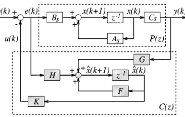
Fig. 1. Block diagram of the closed-loop system with state-estimate feedback controller.

This paper addresses the stability issues of FWL SEFC’s. We derive a tractable measure that quantifies the “robustness” of the closed-loop stability under the controller parameter perturbations, and develop an optimization procedure to search for the optimal controller realizations that maximize the defined measure. The paper is organized as follows. Section II is devoted to formulating the problem to be dealt with and establishing necessary notations. A stability related measure that can be computed easily for a given SEFC realization is given in Section III. The optimal controller realization problem is also defined in this section. In Section IV, the optimization framework for obtaining the optimal FWL controller realization is presented. A numerical example is given in Section V to demonstrate the design procedure and the ef-fectiveness of the proposed optimization method. Some concluding re-marks are given in Section VI.

II. NOTATIONS ANDPROBLEMSTATEMENT

Consider the discrete-time closed-loop system with an SEFC, as shown in Fig. 1. The discrete-time plantP (z), which is assumed to be strictly proper, is represented as

x(k + 1) = Asx(k) + Bse(k)

y(k) = Cs x(k) (1)

withAs 2 Rn2n,Bs 2 Rn2p, andCs2 Rq2n. The discrete-time SEFCC(z) is given by

^x(k + 1) = F ^x(k) + Gy(k) + He(k)

u(k) = K^x(k) (2)

whereF 2 Rn2n,H 2 Rn2p, the control gainK 2 Rp2n, and the observer gainG 2 Rn2q. The representation or realization for a givenC(z) is not unique. In fact, if (F0,H0,K0,G0) is a realization ofC(z), all the realizations of C(z) form a realization set

SC= (F; H; K; G): F = T1 01F0T; H = T01H0;

K = K0T; G = T01_{G0 (3)}

whereT is any real-valued nonsingular matrix, called a similarity trans-formation. Define

w = w1 w2 .. . wN

1 =

Vec(F ) Vec(H) Vec(K) Vec(G)

; w0=1

Vec(F0) Vec(H0) Vec(K0) Vec(G0)

(4)

whereVec(1) denotes the column stacking operator and N = n2+ n(2p + q). Let (A, B, C, D) denote the state-space description of the closed-loop system. It is easy to see that

A(w) = _GCsAs _{F 0 HK}0BsK

= In_{0n T}0n₀₁ A(w0) In_0n 0n_T : (5)

Although different controller realizations yield different A, the closed-loop poles or the eigenvalues ofA, denoted as fig, remain the same; i.e.,i = i(A(w)) = i(A(w0)), i 2 f1; 2; 1 1 1 ; 2ng. In the controller design,(F , H, K, G) will have been chosen to make the closed-loop system stable and, therefore,jij < 1, 8 i.

When a controller realization w is implemented in fixed-point format, it is perturbed into

w + 1w = w1

.. . wN

+ 1w1

.. . 1wN

(6)

due to the FWL effects. Each element of1w is bounded:

(1w)=1 max

i2f1; 111; Ngj1wij 2: (7)

For a fixed-point processor ofBsbits

= 20(B 0B ) ₍₈₎

whereBwis an integer and2B is a “normalization” factor to make the absolute value of each element of20B w no larger than 1. With the perturbation1w, i(A(w)) is moved to i(A(w + 1w)), which may be outside the unit circle. Thus, the closed-loop system designed to be stable may become unstable with an FWL-implemented controller realizationw.

It is, therefore, critical to know when the FWL error will cause the closed-loop system to become unstable. This means to compute the following stability measure [3]

0(w)= inf (1w): A(w + 1w) is unstable :1 (9)

The larger0(w) is, the bigger FWL error the closed-loop stability can tolerate. LetB_sminbe the smallest word length that, when used to implementw, can guarantee the closed-loop stability. Except in simu-lation,B_sminis unknown. An estimate ofB_smincan be provided by

^ Bmin

s0 = Int[0 log2(0(w))] 0 1 + Bw (10) whereInt[x] rounds x to the nearest integer with Int[x] x. From (7)–(10), it can be seen that the closed-loop system is stable whenw is implemented with a fixed-point processor of at least ^Bmin_s0 bits. More-over, as the stability measure0(w) is a function of the controller re-alizationw, we can search for an “optimal” realization that maximizes 0(w):

wopt= arg max

w2S 0(w): (11)

The difficulty with this approach is that computing explicitly the value of0(w) is still an unsolved open problem. Thus, the stability measure 0(w) and the optimization procedure (11) have very limited practical value. An alternative measure that can not only quantify the FWL ef-fects on stability robustness but can also be computed easily must be sought.

III. A TRACTABLESTABILITYRELATEDMEASURE

Roughly speaking, how easily the FWL error 1w can cause a stable control system to become unstable is determined by how close

i(A(w)) are to the unit circle and how sensitive they are to the controller parameter perturbations. Let us consider the following stability related measure:

1(w)=1 min i2f1; 111; 2ng

1 0 ji(A(w))j N

j=1 @i @w_{j w}

(12)

where1 0 ji(A(w))j is called the stability margin of the ith eigen-value. Defining

P(w)= 1w: ji(A(w + 1w))j 0 ji(A(w))j1

(1w) N

j=1 @i

@w_{j w} ; 8 i (13)

we have the following proposition, the proof of which is straightfor-ward.

Proposition 1: A(w + 1w) is stable if 1w 2 P(w) and

(1w) < 1(w).

Remarks: The requirement for1w 2 P(w) is not over-restricted.

In practice, we will only be interested in those 1w that lie in the bounded region:Q(w)= f1w: (1w) < 0(w)g, i.e., those 1w1 that will not cause the closed-loop instability. Since@l=@wjis con-tinuous

l A(w + 1w)

= l A(w) +

N

j=1 C @l @wjdwj

= l A(w) + N

j=1

Re @l

@w_{j a} + i Im @@wl_{j b}

1 1wj (14)

whereC is the oriented segment from w to w + 1w, ajandbjare some points onC. Hence

l A(w + 1w) 0 l A(w)

N

j=1

Re @_@wl

j a + i Im @ l

@w_{j b} 1wj : (15)

Now, let us compare N

j=1

Re @_@wl

j a + i Im @

l

@w_{j b} 1wj

with (1w)

N

j=1 @l

@w_{j w} : (16)

Note that all of theN real-valued items j@l=@wjjwj are in alignment; while theN complex-valued items

Re @l

@w_{j a} + i Im @@wl_{j b} 1wj

are generally out of alignment. Moreover, j1wjj (1w), Re[@l=@wj] and Im[@l=@wj] are differentiable. Thus, a rather large positive exists such that 8 1w 2 f1w: (1w) g

N

j=1

Re @_@wl

j a + i Im @ l

@w_{j b} 1wj

(1w) N

j=1 @l

The above analysis shows thatP(w) exists and at least a large part of Q(w) is covered by P(w).

Generally speaking, there is no rigorous relationship between0(w) and1(w), but 1(w) is connected with a lower bound of 0(w) in some manners. Define

(P(w))=1 inf

1w =2P(w)(1w): (18)

Proposition 2: 1(w) 0(w) if (P(w)) > 0(w).

Proof: From the definition of (P(w)) and the

condi-tion (P(w)) > 0(w), a 1w 2 P(w) exists such that 0(w) = (1w) and A(w + 1w) is unstable. It follows from Proposition 1 that0(w) 1(w).

From Proposition 2, it can be seen that1(w) can be considered as a lower bound of0(w), provided that 0(w) is small enough. The assumption of small0(w) is not too restricted, as it does not make much sense to study the FWL effects on the closed-loop stability for those situations where the closed-loop systems have a very large sta-bility robustness. Most digital control systems do have a small stasta-bility robustness, especially when fast sampling is applied.

To compute1(w), one needs f@i=@wjg, which can be calculated with the following theorem. A proof of this theorem can be found in [4].

Theorem 1: LetA = M0+ M1XM22 Rm2mbe diagonalisable whereX 2 Rl2r, andM0,M1, andM2are independent ofX with proper dimensions. Denotefig = fi(A)g as its eigenvalues. Let xi be a right eigenvector ofA corresponding to the eigenvalue i. Denote Mx= [x1 x2 ; 1 1 1 ; xm] and My= [y1 y2 ; 1 1 1 ; ym] = M0H

x , whereH denotes the transpose and conjugate operation and yiis called the reciprocal left eigenvector corresponding toi. Then

@i

@X =

@i @x11 ; 1 1 1 ;

@i @x1r ..

. ; 1 1 1 ; ... @i

@xl1 ; 1 1 1 ; @i @xlr

= MT

1yi3xTi M2T (19)

where the superscriptT denotes the transpose operator and 3 the con-jugate operation.

Without confusion, we usexiandyito denote the right and recip-rocal left eigenvectors related toi(A(w)), respectively. A(w) can be arranged in the following equivalent forms:

A(w) = _GCsAs 0BsK_0HK + 0n_In F [ 0n In] (20)

A(w) = _GCsAs 0BsK_F + 0n_In H[ 0n 0K ] (21)

A(w) = _GCsAs 0n_F + 0Bs_0H K[ 0n In] (22)

A(w) = As_{0n F 0 HK}0BsK + 0n_In G[ Cs 0n]: (23)

Applying Theorem 1, we obtain @i

@F = [ 0n In]y3ixTi 0n

In (24)

@i

@H = [ 0n In]y3ixTi 0n

0KT (25)

@i

@K = [ 0BsT 0HT] y3ixTi 0n_In (26) @i

@G = [ 0n In]y3ixTi C T s

0n : (27)

For a complex-valued matrixM 2 Cl2r with elementsmij, define a norm ofM as

kMkS=1 l i=1

r

j=1

jmijj: (28)

Then N

j=1 @i

@wj = @@wi _S

= @_@Fi S

+ @_@Hi S

+ @_@Ki S

+ @_@Gi S

: (29)

For a given controller realizationw, the smallest word length B_smin can be estimated with1(w) using the following:

^ Bmin

s1 = Int[0 log2(1(w))] 0 1 + Bw: (30) More importantly, as1(w) is tractable, one can estimate the optimal controller realizations defined in (11) with

^

wopt= arg max

w2S 1(w) (31)

which will be discussed in the next section.

IV. OPTIMIZATIONPROCEDURE

With the computationally tractable stability related measure1(w), we now present a practical optimization procedure to search for an optimal controller realizationwopt^ defined in (31).1 _{Assume that an} initial controller realization (F0, H0, K0, G0) has been provided. For example, the observer gainG0 is obtained using some observer design method with given observer poles, the state-feedback gain K0is obtained using some state-feedback design method with given closed-loop poles, F0 = As 0 G0Cs and H0 = Bs. Let f0i, i = 1; 1 1 1 ; 2ng be the eigenvalues of A(w0), and x0i and y0i be the right and reciprocal left eigenvectors corresponding to 0i, respectively. Partitionx0iandy0i into

x0i= x0i(1)

x0i(2) ; x0i(1); x0i(2) 2 C

n ₍₃₂₎

and

y0i= y0i(1)

y0i(2) ; y0i(1); y0i(2) 2 C

n ₍₃₃₎

respectively. Letw be a controller realization transformed from w0 withT . It is easy to see from (5) that

xi= In_{0n T}0n₀₁ x0i= x0i(1)

T01_x0i(2) (34)

is a right eigenvector ofA(w) corresponding to the same eigenvalue, and

yi= In 0n 0n TT y0i=

y0i(1)

TT_y0i(2) (35)

is the corresponding reciprocal left eigenvector. Substituting (34) and (35) into (24)–(27) yields

@i

@F = TTy30i(2)xT0i(2)T0T (36)

@i

@H = 0 TTy30i(2)x0iT(2)K0T (37)

@i

@K = 0 BTsy30i(1) + H0Ty30i(2) xT0i(2)T0T (38) 1_{In the sequel, by an optimal realization we mean a solution to (31) rather}

@i

@G = TTy0i3(2)xT0i(1)CsT: (39)

We can define (31) in an alternative way:

= _max1

w2S 1(w)

= min T 2R det(T )6=0

max i2f1; 111; 2ng

N

j=1 @i @w_{j w} 1 0 j0ij

= min T 2R det(T )6=0

max i2f1; 111; 2ng

1 @i

@F _S+ @@Hi _S+ @@Ki _S+ @@Gi _S

1 0 j0ij (40)

which means that finding an optimal realization of the SEFC is equiv-alent to obtaining a similarity transformation that is a solution to the following nonlinear optimization problem:

Topt= arg min T 2R det(T )6=0

f(T ) (41)

with the cost function

f(T )=1 max i2f1; 111; 2ng

@i

@F _S+ @

i

@H _S+ @

i

@K _S+ @

i @G _S

1 0 j0ij :

(42)

To find aTopt, we will adopt an iterative optimization procedure to generate a sequencefT0,T1,T2; 1 1 1g, which converges to Topt.

The optimization (41) is constrained. Define= fT 2 R1 n2n: det(T ) = 0g. As is only a manifold in Rn2n_{, starting from aT0 =2} , it is rare for an iterative sequence fTig to move into . Thus, in the iterative procedure, the constraintdet(T ) 6= 0 can practically be ignored, leading to an unconstrained optimization problem:

~ = min

T 2R f(T ): (43)

The possible pitfall of violating the constraint can readily be avoided by the following measure. As the inverse ofT is required in the com-putation off(T ), it is obtained using the singular value (SV) decom-position. If an SV ofT is too small, T is almost singular and a small perturbationInis added toT so that T + In =2 . This small per-turbation, which is rarely needed, will not affect the convergence of the iterative procedure.

Because the cost functionf(T ) is nonsmooth and nonconvex, opti-mization must be based on a direct search without the aid of cost func-tion derivatives. The convenfunc-tional optimizafunc-tion methods for this kind of problem, such as Rosenbrock and Simplex algorithms [10], [11], generally can only find a local minimum. Although the choice of ini-tial realization will not affect the closed-loop eigenvalues, the eigen-value sensitivities@i=@w, 8 i depend on the chosen initial realiza-tion. Thus, for differentw0, the shape of the cost functionf(T ) will change, giving rise to a different degree of difficulty in the optimization procedure. It is therefore important to use an efficient, and preferably global, optimization method. We adopt a global optimization strategy based on the adaptive simulated annealing (ASA) [12], [13] to search for a true global optimumwopt^ .

V. ILLUSTRATIVEEXAMPLE

This section presents a numerical example to illustrate the design procedure and how the proposed optimization approach can be used effectively to search for the optimal FWL realization of SEFC’s. This example was taken from [9]. The discrete-time plantP (z) was given by

As=

2:758 200e + 0 02:534 177e + 0 7:755 853e 0 1

1 0 0

0 1 0

Bs= 1 0 0

Cs= [ 2:200 000e 0 3 4:400 000e 0 3 2:200 000e 0 3 ]:

The initial realization of the controllerC(z) was chosen to be

F0=

2:497 941e + 0 03:054 695e + 0 5:153 264e01 7:776 040e01 04:447 920e01 02:223 960e01 01:801 490e01 6:397 019e01 01:801 490e01

H0= 1 0 0

K0= [ 4:761 000e 0 1 08:183 439e 0 1 3:505 623e 0 1 ]

G0=

1:182 995e + 2 1:010 891e + 2 8:188 593e + 1

:

The corresponding transition matrixA(w0) was formed, from which the poles and eigenvectorsf0j,x0j,y0j,j = 1; 1 1 1 ; 6g of the ideal closed-loop system were computed.

The ASA algorithm was used to search for anToptby solving the optimization problem (41), and it produced the following solution:

Topt=

02:492 226e + 2 08:436 334e + 1 2:500 780e + 2 01:712 397e + 2 06:278 793e + 1 2:126 909e + 2 09:225 780e + 1 03:503 457e + 1 1:704 995e + 2

:

This gave rise to the optimal FWL controller realizationwopt^ :

Fopt=

7:273 562e01 01:063 087e01 1:577 498e01 01:906 839e01 6:591 385e01 2:312 892e01 7:272 022e02 03:150 339e02 4:865 053e01

Hopt=

05:926 328e 0 2 1:743 758e 0 1 3:763 549e 0 3

Kopt= [ 01:086 402e + 1 01:065 065e + 0 4:778 530e + 0 ]

Gopt=

01:558 451e 0 3 6:013 747e 0 2 4:917 847e 0 1

:

TABLE I

COMPARISON OF STABILITY RELATED

MEASURES, ESTIMATEDMINIMUMBITLENGTHS ANDTRUEMINIMUMBIT LENGTHS FOR THEINITIAL ANDOPTIMALCONTROLLERREALIZATIONS

minimum bit lengths for the initial and optimal controller realizations. It can be seen that, for this example, the optimization achieved an im-provement by a factor of 30 on the closed-loop stability related measure and an 8-bit reduction in the required minimum bit length.

VI. CONCLUSIONS

In this paper, we have presented an approach to address the stability issues of the closed-loop discrete-time system where a state-estimate feedback controller is implemented with a fixed-point processor. An FWL closed-loop stability related measure has been derived, which is computationally tractable. As this measure is a function of the con-troller realization; the optimal realization problem of state-estimate feedback controllers is to find a realization that maximizes this mea-sure. It has been shown that this optimal realization problem can be interpreted as a nonlinear programming problem. An efficient global optimization strategy based on the ASA algorithm has been adopted to solve this nonsmooth and nonconvex optimization problem.

REFERENCES

[1] P. Moroney, A. S. Willsky, and P. K. Houpt, “The digital implementation of control compensators: The coefficient wordlength issue,” IEEE Trans.

Automat. Contr., vol. AC-25, pp. 621–630, Aug. 1980.

[2] M. Gevers and G. Li, Parameterizations in Control, Estimation and

Fil-tering Problems: Accuracy Aspects. London: Springer Verlag, 1993. [3] I. J. Fialho and T. T. Georgiou, “On stability and performance of sampled

data systems subject to word length constraint,” IEEE Trans. Automat.

Contr., vol. 39, pp. 2476–2481, Dec. 1994.

[4] G. Li, “On the structure of digital controllers with finite word length con-sideration,” IEEE Trans. Automat. Contr., vol. 43, pp. 689–693, 1998. [5] R. H. Istepanian, G. Li, J. Wu, and J. Chu, “Analysis of sensitivity

mea-sures of finite-precision digital controller structures with closed-loop stability bounds,” Proc. Inst. Elect. Eng. Contr. Th. Applicat., vol. 145, no. 5, pp. 472–478, 1998.

[6] S. Chen, J. Wu, R. H. Istepanian, and J. Chu, “Optimizing stability bounds of finite-precision PID controller structures,” IEEE Trans.

Au-tomat. Contr., vol. 44, pp. 2149–2153, Nov. 1999.

[7] R. H. Istepanian, J. Wu, J. F. Whidborne, J. Yan, and S. E. Salcudean, “Finite-word-length stability issues of teleoperation motion-scaling con-trol system,” in Proc. UKACC Contr.’98, Swansea, UK, Sept. 1–4, 1998, pp. 1676–1681.

[8] T. Kailath, Linear Systems. Englewood Cliffs, NJ: Prentice-Hall, 1980. [9] G. Li and M. Gevers, “Optimal finite precision implementation of a state-estimate feedback controller,” IEEE Trans. Circuits Syst., vol. 37, pp. 1487–1498, 1990.

[10] G. S. G. Beveridge and R. S. Schechter, Optimization: Theory and

Prac-tice. New York: McGraw-Hill, 1970.

[11] L. C. W. Dixon, Nonlinear Optimization. London: English Universi-ties Press, 1972.

[12] L. Ingber, “Simulated annealing: Practice versus theory,” Math. Comput.

Model., vol. 18, no. 11, pp. 29–57, 1993.

[13] S. Chen and B. L. Luk, “Adaptive simulated annealing for optimization in signal processing applications,” Signal Process., vol. 79, no. 1, pp. 117–128, 1999.

Practical Stability and Stabilization Luc Moreau and Dirk Aeyels

Abstract—We present a practical stability result for dynamical systems

depending on a small parameter. This result is applied to a practical sta-bility analysis of fast time-varying systems studied in averaging theory, and of highly oscillatory systems studied by Sussmann and Liu. Furthermore, the problem of practically stabilizing control affine systems with drift is discussed.

Index Terms—Approximation methods, Lie algebras, stability, time-varying systems.

I. INTRODUCTION

In the present note, dynamical systems that depend on a small pa-rameter are studied from the viewpoint of continuity of solutions.

Consider a system that depends on a small parameter" > 0

_x = f"_{(t; x) (1)}

and a system

_x = g(t; x) (2)

with the assumption that trajectories of (1) converge—uniformly on compact time intervals—to trajectories of (2) as" # 0.

A particular example is given by fast time-varying systems studied in averaging theory

_x = f t_"; x : (3)

It is well known that, under appropriate technical conditions, there ex-ists an associated averaged system

_x = fav(x) (4)

such that trajectories of (3) converge—uniformly on compact time in-tervals—to trajectories of (4) as" # 0.

Teel et al. [1] have proven that, under appropriate technical condi-tions, if the origin of the averaged system (4) is a globally asymptot-ically stable equilibrium point, then the fast time-varying system (3) is practically stable. Their proof is based on advanced Lyapunov tech-niques.

In the present note, it is recognized that this practical stability re-sult is of a topological nature, that it is a consequence of the conver-gence property of solutions: we prove the general result that, under ap-propriate technical conditions, if the origin of system (2) is a globally uniformly asymptotically stable equilibrium point, then system (1) is practically stable. This approach provides an alternative proof for the practical stability result [1] mentioned above, and extends it to a larger class of systems: it is not only applicable to fast time-varying systems as in averaging theory, but also, for example, to highly oscillatory sys-tems studied by Sussmann and Liu [2]. This latter application is useful for control purposes. Indeed, it leads to a practical stabilization algo-rithm for a class of control affine systems with drift.

An outline of this note is as follows. Section II introduces some notations and hypotheses. Section III introduces a notion of practical

Manuscript received April 8, 1999; revised November 29, 1999. Recom-mended by Associate Editor, W. Lin. The work of L. Moreau was supported by BOF Grant 011D0696 of the Ghent University.

The authors are with the SYSTeMS Group, Ghent University, Technolo-giepark 9, 9052 Zwijnaarde, Belgium (e-mail: [email protected]).

Publisher Item Identifier S 0018-9286(00)06078-5.