By Kien-Tsoi T.E. Tjin-Kam-Jet
Master’s thesis University of Twente
March 2009
Graduation committee:
Chairman: Dr. ir. Djoerd Hiemstra
1st coordinator: Pavel V. Serdyukov, Msc.
- i -
Abstract
Centralized Web search has difficulties with crawling and indexing the Visible Web. The Invisible Web is estimated to contain much more content, and this content is even more difficult to crawl.
- iii -
Preface
During my Final Project, I was still on the board of the classical student choir of the Twente University. My last project as a member of the board involved co-organizing a one-day event where everybody could rehearse, relax and have fun, and give a public performance on stage in the evening. This project received the Student Union Culture prize, which is a very nice way to end my membership of the board, and my time as a student.
While looking for a suitable Final Project, I was leaning towards a project that involved Database technology and Natural Language Processing. A logical step was to discuss my plans with my study advisor, Djoerd Hiemstra. I found his suggestion for doing a Final Project on distributed Web search very appealing and so he became my supervisor. Soon, it became apparent that I should pursue a different direction in the name of Machine Learning, which I first had to become more acquainted with. This field is very interesting, although it would not have been that interesting were it not for the discussions I had with a fellow student, Edwin de Jong.
Working on this research project was very inspiring, not just because of the topic, but also because of the open and friendly research environment.
I would like to thank my supervisors for their guidance and valuable input in my research. I would also like to thank Ander de Keijzer, for providing me with an account on his fast machine. I would also like to express my gratitude to everyone who gave me advice and useful comments, especially, Robin Aly, my fellow lab rats, and Wolter Siemons. Special thanks to my girlfriend, who supported me throughout this project.
- v -
Contents
1 Introduction ... 1
1.1 Motivation...1
1.1.1 Search Aspects...1
1.1.2 Web Search Issues ...1
1.1.3 Metasearch ...2
1.2 Research Focus ...2
1.3 Research Questions ...3
1.4 Thesis Outline ...4
2 Ranking in Information Retrieval ... 5
2.1 Introduction...5
2.2 Term Weighting; an Example...5
2.3 Distributed Collection Statistics ...6
2.4 Learning to Rank ...7
2.4.1 Discriminant Functions ...7
2.4.2 Linear Support Vector Machines ...8
2.4.3 Non-Linear Separable Data...10
2.4.4 Non-Linear Support Vector Machine ...11
3 Related Work on Result Merging ... 13
3.1 Introduction...13
3.2 Merging Strategies ...13
3.2.1 Normalizing Scores ...13
3.2.2 Clustering Techniques...14
3.2.3 Combining Evidence ...14
3.2.4 Regression Models...15
3.2.5 Experts and Voting ...16
3.2.6 Download and Rank ...16
3.2.7 Learning to Rank...16
3.3 Uncooperative Environments...16
3.4 Summary ...17
4 Research Methodology ... 19
4.1 Dataset...19
4.1.1 Creating Subcollections and their Result Pages...19
4.1.2 Selection Policies ...22
4.2 SVM Models for Result Merging...23
4.2.1 Features ...23
4.2.2 Preference Pair Constraints ...24
4.2.3 Preference-SVM Labeling ...25
- vi -
4.2.5 Model Settings ...26
4.3 External Influences...27
4.3.1 Number of Result Lists...27
4.3.2 Subcollection Size...28
4.3.3 Search Engine Selection Policy ...28
4.4 Evaluation ...28
4.4.1 Evaluating SVM Models ...28
4.4.2 Evaluating Retrieval Performance ...29
5 Results ... 31
5.1 Preliminary Test Results...31
5.2 Centralized Baseline Performance ...32
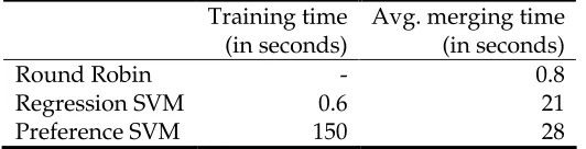
5.3 Training Time and Merging Time ...32
5.4 Important Features ...33
5.5 RR & SVM Performance...33
6 Discussion... 41
6.1 More on the Results...41
6.2 Kernels and Overfitting...41
6.3 Similar Regression and RR Behavior ...42
6.4 Efficient Result Set Selection...42
6.5 LMAP...43
6.6 Preference-SVM ...43
7 Conclusion ... 45
8 Future Work ... 47
9 Bibliography... 49
- 1 -
Chapter 1
Introduction
Finding relevant information on the Web is becoming more important and increasingly more challenging. This chapter exposes the problems with the current state of Web search and introduces a potential solution.
1.1 Motivation
1.1.1 Search Aspects
Every day millions of people all over the world use search engines. A search engine can only provide relevant results if it already has some information about the Web. It obtains this information by downloading Web content. Then, it orders this information, for instance, by means of an inverted file [2], to facilitate quick retrieval of relevant results. Finally, users must somehow be allowed to search within this knowledge. These search aspects are typically referred to as: 1) crawling (a structured way of collecting Web content), 2) indexing (ordering the content for efficient and quick retrieval), and 3) searching.
1.1.2 Web Search Issues
Dominant search engines such as Google, Yahoo!, and Live Search, control all search aspects and store their index in a centralized manner. Even though they use multiple machines to crawl, index, and search the Web, these search engines are still called centralized because; first, they control all search aspects (from one location); second, their machines have complete access to their crawled Web statistics, allowing them to build a true global (centralized) index, as opposed to building many (decentralized) local indices, one for each machine that crawled a piece of the Web. Limitations regarding the centralized index paradigm will be discussed next.
1.1.3 Metasearch
Metasearch, a form of distributed Web search, potentially solves the problems outlined in the previous section. A metasearch system contains multiple search engines and at least one search broker. Each search engine indexes a distinct part of the Web whereas the broker mediates between the user and these different search engines. At query time, the user sends a query to the broker, upon which the broker chooses the best search engines and forwards this query to these engines. Each search engine retrieves its most relevant results and sends these results to the broker. The broker merges these results into one result list and presents this to the user. Generally, the broker only controls the way the search engines are selected and the way their results are merged, it has no control over the internals of each search engine.
We propose a solution where specifically as many as possible Web hosts index their own content and thus become a (small) search engine. The key benefits of this approach include no or less crawling, as all or most servers index their own local content; more Web coverage; and more specialized search engines: these can be thought of as indexing structured data which would otherwise be hidden (e.g., inside the Deep Web), or which are specialized in finding relevant documents about a certain topic.
Before metasearch can be made operational, Callan [9] identified three major problems which must be solved first:
1. Resource description: describing the contents of each database;
2. Resource selection: given an information need and a set of resource descriptions,
a decision must be made about which databases to search; and,
3. Result merging: integrating the ranked lists returned by each database into a single, coherent ranked list.
A resource description is often some kind of an excerpt of a database’s index; it informs about the (estimated) number of different words in the index and how frequent these words appear in (some part of) the database.
A selection method is for example to treat each resource as one very large document and then to select that document with the highest query-term occurrence.
Simple methods for merging results are for instance to concatenate all results serially, or
to combine the results in a Round Robin1 (RR) fashion.
This research project is part of a bigger project on distributed Web search at the Twente University and focuses on the third problem of result merging.
1.2 Research Focus
This research aims at improving the efficiency and the performance of result merging methods. When a query is issued, we tackle the efficiency problems by restricting ourselves to use information only from the returned result pages, instead of downloading the documents either partially or completely. The simplest method using only such information is RR merging.
The problem of result merging can be viewed as that of re-ranking a set of ranked results. Ranking often involves combining multiple “sources of information” (e.g., the
length of a document, the frequency of a word, the amount of similar terms in the query and the title, etcetera), which we call features. Not all features contribute equally to the result; they are often weighted.
Manual weighting becomes infeasible when dealing with many information sources. With enough computing resources and training data, techniques from the field of Machine Learning (ML) allow us to learn these weights automatically.
ML techniques are often used for classification and regression tasks. Nallapati [24], classifies documents as relevant or irrelevant. Others, [5, 13, 16, 18], classify pairs of documents (preference pairs), thereby indicating which document is more preferred (relevant) than the other. Finally, some researchers [26, 33] use regression to estimate global document ranks.
The Support Vector Machine (SVM) [39], a particular ML-technique, can be used for both classification and regression. It was shown that the SVM (trained on partial preference rankings) could be used to optimize the performance of a broker system and it even outperformed Google [18].
We will use the term preference-SVM to refer to the case where a classification model is trained on preference-pairs; and we will use the term regression-SVM to refer to the case where a regression model is trained on single training instances, not on pairs.
1.3 Research Questions
The main question this research will answer is:
Q1. Which of RR-merging, preference-SVM, and regression-SVM is recommended and why?
For efficiency reasons, the solution to the result merging task is restricted at query-time: we are only allowed to download the result lists from a search engine, not the actual documents. However, since the broker first selects a number of search engines before merging their results, it must have some information about which engines are most capable of answering the query. We assume that this information is also available at query-time. Thinking in term of features, the next question is:
Q2. Using only information from the result lists and the broker’s selection mechanism, what are suitable features to use for result merging, and what are their weights?
It might happen that the broker selects a sub-optimal set of search engines, where, for example, the set contains too few engines that return relevant results. Ideally, the result merging strategies should produce a good ranking even with a sub-optimal set of search engines. This brings us to our next question:
Q3. How vulnerable are the merging strategies to external influences like the number of result lists to merge, or the quality of the result lists?
Efficiency is gained by not downloading documents at query time. However, a more concrete indication of efficiency would be desired. The final question is:
1.4 Thesis Outline
The following chapter introduces the ranking problem in Information Retrieval; it shows how features are generally used and aggregated in order to derive a ranking. Then, it introduces a specific approach for solving the ranking problem, called Learning to Rank, where it formally introduces the Support Vector Machine.
- 5 -
Chapter 2
Ranking in Information Retrieval
Introduces necessary concepts to build upon and improve state-of-the-art ranking in IR.
2.1 Introduction
Information Retrieval concerns itself with the situation where a user, having some information need, performs queries on a collection of documents to find a set of relevant documents where the most relevant ones are ranked highest [15].
Traditionally, in (an) Information Retrieval (engine), documents are represented as a Bag of Words (BW) where the meaning of the document is simply seen as the collection of words it contains. This representation discards properties such as the structure of the text, word order, and much more. Furthermore, words in the document are often stemmed and this is optionally followed by removal of stop-words (e.g., non-content bearing words such as a, the, who), creating a bag of index terms. Likewise, the same pre-processing can also be applied to the user’s query. Retrieval based on index terms fundamentally assumes that the semantics of the document and of the user information need can be expressed by sets of index terms [2].
Having representations of both query and document, the next step is to determine which documents are more likely to be more relevant to a given query. Today, almost all IR systems compute a single numeric score indicating how well a document matches the query. This is the result of aggregating values of features related to the document and/or the query terms. For example, term frequency, document frequency and document length are the main features used in many prominent (BW-based) IR models such as the Vector Space Model (VSM) [31], the Okapi BM25 probabilistic model [30] and language models [12, 20, 28]. To illustrate how features contribute to the computation of relevancy, an example will be discussed in the following section using the VSM.
2.2 Term Weighting; an Example
In the VSM, documents and queries are represented as feature vectors of terms that occur within the collection. The value of each element (feature) within the vector is called the (term) weight and is generally closely related to the term’s frequency (TF) within the document.
Let us start with a simplified example. Imagine a salad recipe (i.e., a document) containing the four terms cabbage, tomato, fried, and bacon with term frequencies 3, 4, 2, and 5 respectively. Let us assume that our whole collection of documents contains only
these four terms and that we put these features in the above order. This (i-th) document d
)
5
,
2
,
4
,
3
(
=
id
r
Queries can also be represented in the same way. For instance, the query q for fried bacon would be represented as:
)
1
,
1
,
0
,
0
(
=
q
r
In the VSM, it is instructive to view both the documents and the queries as points (vectors) in a multidimensional space; the feature-values (or term weights) are the coordinates, and each feature is a different dimension. The intuition is that documents residing near the query can be seen as more relevant than documents that are farther away. Notice how the VSM does not define relevancy as a binary “yes” or “no”. Instead, it specifies a distance between two objects where a shorter distance is assumed to imply higher similarity (and in this case, higher relevancy). The standard way of measuring the distance between these vectors is by taking the cosine of the angle between the object’s vectors (Equation 2.1). As a result, similar objects will have a cosine similarity (sim for short) of one, while orthogonal objects (having no terms in common) will have a cosine of zero.
∑
∑
∑
= j j D j j Q j D j j Q i i i W W W W D Q sim 2 , 2 , , , ) , ( (2.1)Of course, some terms may be more helpful than others may when determining the relevancy of a document to a given query. Terms appearing in only a few documents are more useful (in discriminating those few documents from other documents) than terms occurring in many documents across the collection. Weighting terms with their Inverse Document Frequency (IDF) is one way of indicating their discriminative power. The IDF of term ti is simply the ratio N / ni, where N is the total number of documents in the
collection and ni is the number of documents in which term ti occurs. This form of
combining TF with IDF is called TF.IDF weighting.
2.3 Distributed Collection Statistics
Collection statistics such as TF and IDF play a non-trivial role in discriminating relevant from irrelevant documents. TF.IDF somewhat samples the (importance of the) content of a web page. Other statistics such as PageRank [25], measure the quality and popularity of a web page. Note that for these statistics to achieve good performance, the collection information should be as complete as possible.
Whereas centralized IR has the luxury of gathering all crawled collection statistics at a central location, distributed IR simply cannot. If a search broker would gather all collection statistics of all remote search engines, besides almost becoming centralized IR, it would also involve huge amounts of bandwidth, definitely even more than centralized IR.
To minimize the network bandwidth consumption, the broker’s problem of obtaining
representative collection statistics should be solved for instance by using highly
search engines in their probability of returning most relevant results. QBS is also useful for result merging as can be seen in Chapter 3.
2.4 Learning to Rank
IR models with few parameters, such as the Okapi BM25, allowed researchers to hand-tune the model. However, fine-tuning features by hand becomes impossible when using many more features. Fortunately, with the recent availability of large standardized test
corpora1 and cheap computing resources, fine-tuning the features automatically has
become possible.
Given a set of examples, the idea of Learning to Rank is to find those characteristics that can distinguish the good ones from the bad ones. Based on those characteristics, we should subsequently be able to predict whether new examples are good or bad.
Learning to Rank (LETOR) is a new and popular topic, both in Machine Learning (ML) and in Information Retrieval. In LETOR, the ranking problem is often formulated as a classification problem. We distinguish two subcategories: one (point-wise), a single document is classified as either relevant or not relevant; two (pair-wise), a pair of documents is classified, indicating which of the two documents is more preferred.
Close attention will be paid to the Support Vector machine (SVM) [39], which enjoys much popularity and is often reported with successful results. SVMs are a family of linear discriminant functions and are used for both classification and regression. A fact about SVMs is that they always find a global solution in contrast to neural networks, where many local minima usually exist [8].
Using point-wise classification, Nallapati [24] showed that SVMs are on par with state-of-the-art language models. A number of studies experimented with pair-wise classification, for instance [5, 13, 16, 18].
An SVM model is trained on some data sample S = {(xt, rt)| xt∈ℝn, rt∈Y}, where xt is an
n-dimensional feature vector2 representing instance t, and rt is the assigned label. We
distinguish between classification if Y is a finite unordered set (nominal scale), and between regression if Y is a metric space, for example, the set of real numbers. The following subsections are mainly intended to give you an idea of what a support vector machine is and what it does.
2.4.1 Discriminant Functions
The simplest classifier is a linear classifier. A linear binary classification can formerly be written as sign(f: X ⊆ ℝn → ℝ), with X a set of n-dimensional input data. So, each
element x∈X receives a positive label if f(x) ≥ 0, and a negative label otherwise. In linear classification, f(x) should be linear. For instance, it could be written as the dot product of the weight vector and the input vector, plus a constant:
f(x) = 〈w, x〉 + b
1 A collection of many documents and queries; for each query a number documents are judged by a group of people as being relevant or not relevant.
We must learn the right values of the parameters (w, b), since these control our decision rule. In Figure 2.1, the thick line is a separating hyperplane as it separates the two classes x and o. It can also be seen that there are many possible separating hyperplanes. However, we want the hyperplane with the best generalizability, so that when given unseen data, it will most often produce the right classification.
Figure 2.1: A two-dimensional space containing two linearly separable classes
A hyperplane could be chosen with the biggest distance to its surrounding data points. The distance from the closest point to the hyperplane is called the margin and so this hyperplane is called the maximal margin hyperplane.
2.4.2 Linear Support Vector Machines
Any hyperplane can be written as the set of points X satisfying 〈w, xt〉 + b = 0. Here, w is
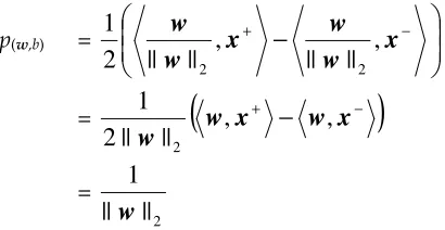
the hyperplane’s normal vector, that is, it is perpendicular to the hyperplane. We want to choose (w, b) such as to maximize the margin p(w,b) between the farthest possible parallel
hyperplanes that still separate the data (see the dashed lines parallel to the hyperplane in Figure 2.1).
The canonical hyperplane is obtained by scaling (w, b) so that for the nearest point |〈w,x〉 + b| = 1 holds. Note that, if the data is linearly separable, the distance between the two parallel hyperplanes is 2. The margin is given by:
p(w,b) =
−
−+
x
w
w
x
w
w
,
||
||
,
||
||
2
1
2 2
=
(
w
x
+−
w
x
−)
w
||
,
,
||
2
1
2= 2
||
||
[image:16.595.199.404.633.739.2]We can maximize the margin by minimizing the Euclidean norm
w
2. One of the reasons to prefer a maximal margin is the underlying assumption that both training and test data are drawn from the same distribution. Therefore, we could reasonably assume that a test point would be near a training example. If every test point is a maximum distance r≥ 0 away from a training point, then all test points will be classified correctly if we have a margin p(w,b) > r.When given a linearly separable data set S = {(x1, r1)… (xk, rk)}, the (canonical) hyperplane
(w, b) that solves the primal optimization problem
minimizew,b
2
1
2
w
, (2.2)with rt (〈w, xt〉 + b) ≥ 1, t = 1… k.
will be a maximal margin hyperplane with margin p(w,b) =
2
||
||
1
w
.In practice, researchers will often work on the dual representation1, a Lagrange formulation of the problem. The reasons for doing this are two-fold. First, the constraints in (2.2) will be replaced by constraints on the Lagrange multipliers themselves. Second, the optimization problem can be expressed as dot products of its input vectors, such as in Equation 2.3. This makes it possible to apply the kernel trick, allowing us to train non-linear SVMs.
The dual optimization problem is a maximization problem:
maximize W(αααα) =
∑
∑
= =
−
k i k j i j i j i j ii
r
r
1 , 1
,
2
1
x
x
α
α
α
, (2.3)with
0
1
=
∑
= k i i ir
α
,0
≥
i
α
, i = 1..kNote that there is a Lagrange multiplier αi for each training point. In the solution, the points for which αi > 0 lie on (one of) the hyperplanes and are called support vectors, as they ‘support’ the hyperplane. All other training points have αi = 0.
Given a solution αααα` to the optimization problem and given a new data point x, the choice which class to assign to x is obtained by taking its dot product with all the support
vectors (remember that the αi for the non-support vectors is zero anyway):
+
=
∑
=`
,
`
sgn
)
(
' 1b
f
s sv i i ii
x
x
x
α
γ
where
b` =
2
)
,
(
min
)
,
(
max
ri=−1w`
x
i+
ri=1w`
x
i−
w` =
∑
=
k
i
i i i
r
1
`
x
α
2.4.3 Non-Linear Separable Data
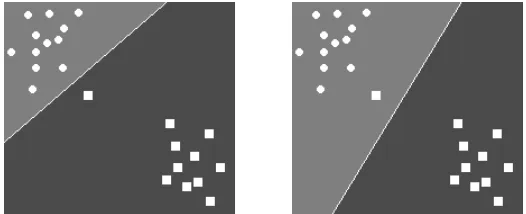
Up until now, we have been assuming (noise free) linearly separable data, in which case it makes sense to choose a maximal margin classifier. As can be seen in Figure 2.2, a maximal margin classifier is not always the best option if the data contains noise (in this case, the noise is in the form of an outlier).
With non-linear separable data, a classification such as in Figure 2.3 will never be found by a maximal margin classifier because the constraint in Equation 2.2, that all data points should be classified correctly, is too strict.
Figure 2.2: The left figure shows a maximal margin classification. The right figure has one misclassification, but is probably more desired. Based on similar figures in Wellens [43].
Figure 2.3: This classification cannot be made by our current maximal margin classifier because the data is not linearly separable. Based on similar figures in Wellens [43].
As can be seen in Figures 2.2 and 2.3, by allowing some errors, we can still make desired linear classifications. The constraints should somehow be relaxed. That is why Cortes and Vapnik [14] introduced positive slack variables:
0
≥
t
ξ
, t = 1 ... kwhich result in the following (weaker) constraints:
[image:18.595.166.429.305.412.2] [image:18.595.237.357.455.565.2]Each training instance gets a slack variable in such a way that the constraint is satisfied. Because of allowing classification errors, the margin would become infinite. Thus, the optimization problem should be modified to include a penalty for each error:
minimizew,b
2
1
2
w
+ C∑
=
k
t t 1
ξ
(2.4)with rt (〈w, xt〉 + b) ≥ 1 - ξt,
ξt≥ 0, t = 1 … k
Here, C is a user-specified parameter and should be greater than 0. A bigger C means higher penalty on classification errors. Note that this algorithm will usually not result in a maximal margin classifier, which is why this is called a soft margin classifier.
The dual of Equation 2.4 is given by:
maximize W(αααα) =
∑
∑
= =
−
k i k j i j i j i j ii
r
r
1 , 1
,
2
1
x
x
α
α
α
, (2.5)with
0
1
=
∑
= k i i ir
α
,0
≥
≥
iC
α
, i = 1..kwhich is very similar to that of the maximal margin SVM in Equation 2.3.
2.4.4 Non-Linear Support Vector Machine
Perhaps the biggest showpiece of the SVM is that it can project the data points to some higher dimensional feature space and find a linear (soft margin) classification; usually corresponding to a non-linear classification in the input space. Kernels are used as the projection mechanism. Furthermore, kernels allow computational tractability when working in high or infinite-dimensional spaces.
Definition 1 (Kernel). A kernel is a function K, such that for all x, y∈X⊆ℝn
)
(
),
(
)
,
(
x
y
=
Φ
x
Φ
y
K
,where Φ is a projection from input space X to feature space H.
Substituting the dot product for a kernel in Equation 2.5 yields the following optimization problem:
maximize W(αααα) =
∑
∑
= =
−
k i k j i j i j i j ii
r
r
K
1 , 1
)
,
(
2
1
x
x
α
α
α
, (2.6)with
0
1
=
∑
= k i i ir
α
,0
≥
≥
iIt is possible to encode extra a-priori knowledge in a kernel such that it can be used as a similarity measure. Even though kernels may differ, they should often be able (if they work well) to find roughly the same regularities in the given training data. This does not imply that it does not matter what kernel you use.
Next, the concept of the capacity of a learning machine, that is, its ability to learn any training set without error, will be explained by means of an example taken from Burges’ tutorial on SVMs [8]. A machine with too much capacity is like a botanist with a photographic memory who, when presented with a new tree, concludes that is not a tree because it has a different number of leaves from anything she has seen before; a machine with too little capacity is like the botanist’s lazy brother, who declares that if it’s green, it’s a tree. Neither can generalize well.
Intuitively, the use of a kernel will often be in accordance with increasing the capacity of the classifier.
When using SVMs for classification, two parameters must be specified: the trade-off
parameter C, and the kernel. However, depending on the kernel, some additional
parameters may have to be specified.
Examples of kernels:
1. Linear kernel:
K
(
x
,
y
)
=
x
,
y
2. Homogeneous polynomial kernels:
K
(
x
,
y
)
=
x
,
y
d3. Inhomogeneous polynomial kernels:
K
(
x
,
y
)
=
(
x
,
y
+
c
)
d4. Gaussian radial basis function (RBF) kernel:
K
(
x
,
y
)
=
exp
(
−
γ
x
−
y
2)
The linear kernel requires no additional parameters. The homogeneous polynomial
kernel has one additional parameter d. The inhomogeneous polynomial kernel has two
- 13 -
Chapter 3
Related Work on Result Merging
3.1 Introduction
The task of merging multiple result lists into a single ranked list is called result merging [33]. The result-lists are usually obtained by sending the same information need (often
the same query) to N different (remote) search engines. There are no restrictions on the
overlap-rates between the document collections of the different search engines, nor are there any restrictions on what ranking functions should be used.
The problem of result merging is not new and it has been a major open problem in distributed IR since around 1994 [33, 35].
Many terms have been used to refer to the problem of result merging, for example, data-, collection-, results-, information-fusion, and query-combination. Query combination is a more restricted definition of result merging. Particularly, it addresses the effect of merging result lists of different formulations of the same information problem to the same search engine [6]. This can be seen as a variant of query expansion where instead of producing a longer query, a set of N similar queries is produced. This set of N queries is sent to the same IR system and the resulting N result lists are then combined by, for example, using the weighted sum of the similarity scores.
Round Robin (RR) merging was briefly mentioned in Chapter 1. Because of its simplicity, it is often used as a baseline for merging experiments. RR merging is defined as follows: given n result lists L1,L2…Ln, take the first result r1 from each list Li as the first n results,
then, take the second result r2 from each list as the next n results, and so on. RR merging
produces a list: L1r1,L2r1…Lnr1, L1r2,L2r2…Lnr2, L1r3,L2r3…Lnr3, etcetera.
Often, the rank of the results is the only feature used when doing RR merging. The assumption is that all result lists have an equal distribution of relevant documents and that most relevant documents are ranked highest. However, any additional information about the relevant document distributions of the servers can be used to rank the servers. Having these two features, the rank of both the server and its results, RR will not blindly pick the next best result from a random server; it will pick the next best result from the next best server.
3.2 Merging Strategies
3.2.1 Normalizing Scores
Search engines supplied numeric scores indicating how well the document matched the query, which enabled raw score merging. However, document scores from different search engines may often not be directly comparable. Normalizing statistics such as Inverse Document Frequency (IDF) could be a solution. The idea is that normalizing would achieve the same performance as when all different collections were combined in one global collection and then queried. Normalizing document scores entails significant communication and computational costs when collections are distributed across a wide-area network. Therefore, instead of normalizing the scores, one could weight them. Weights could be based on the document’s score and/or the collection ranking information. Callan et al. showed that the performance of weighted score merging was as effective as normalized score merging, the other two approaches were significantly worse.
3.2.2 Clustering Techniques
Also around 1995, Voorhees et al. [42] developed two merging strategies that are independent of the IR-model of the different search engines. They defined the collection fusion problem as finding the values λ1 ... λc, that maximize
∑
==
c i iN
1λ
and(
)
1 t c t I Q t
F
λ
∑
=Here, N is the desired amount of documents to be retrieved, FIQ(x) models the relevant
document distribution of search engine I for query Q given x, the amount of documents
to be retrieved. In practice, FIQ is not known and must be approximated. Their first
strategy models relevant document distributions; the k most similar queries are used to
learn a model of the relevant document distribution for each search engine I. These
models are then used in a maximization procedure to learn the values λi. They use the
VSM to compute similarities between queries. Their second strategy creates query clusters based on the amount of common documents retrieved, and assigns weights to these clusters. At query time, the most similar cluster to the query is selected from each search engine. Each cluster’s weight, relative to the sum of all retrieved weights, determines the amount of documents to be retrieved from each search engine. Both strategies only determine the amount of documents to retrieve from each search engine. A total ordering on the result set is imposed either in a Round Robin fashion, or by
chance: to select the document for rank r, a search engine is chosen by rolling a C-faced
die that is biased by the number of documents still to be picked from each of the C search
engines. The next document from that search engine is placed at rank r and removed from further consideration.
They show that these fusion techniques can approximate the performance of a single collection run at the ranks that will be of interest to the user.
3.2.3 Combining Evidence
In 2001, Rasolofo et al. [29] experimented with a current news metasearcher using low cost merging methods. They noted important differences between their news meta-searcher and a metameta-searcher of conventional search engines, one of which is:
Their main merging approach was based on document scores, called raw-score merging. However, it was not practical since the document scores were seldom reported and they would not be comparable anyway due to differences in indexing and retrieval strategies used by the servers.
Therefore, they employed a generic scoring function that returns comparable scores
based on various document fields (such as, title, summary, or date). For each document i
belonging to collection j for the query Q, they compute a weight, denoted wij as follows:
2 2 q
LF
NQW
i i ij
L
w
+
=
here, NQWi is the number of query words appearing in the processed field of the
document i, Lq is the length (number of words) of the query, and LFi is the length of the
processed field of document i.
They define several merging alternatives:
• their first alternative, which is also their baseline, is to apply RR merging based
only on the ranks defined by the servers, denoted simply as RR;
• their second alternative is to first compute a score for each document using the
XX field with their generic scoring function, and then adopt the raw-score merging approach. They denoted this alternative as SM-XX;
• their last alternative is to re-rank the results of each server using their generic scoring function, and then use the RR merging. This is denoted as RR-XX.
The scores are based on a combination of easily extractable information from result lists like: rank, title, summary, date. Additionally, they included estimated server usefulness and estimated collection statistics. Their best merging scheme (a raw-score merge based on a combination of estimated server usefulness, title and summary score) worked almost as well as merging based on downloading and rescoring the actual news articles.
3.2.4 Regression Models
result list. Once all remote result lists have been complemented with estimated document scores, they proceed just as Si and Callan [33] to map search-engine-specific document scores onto the centralized sample index’s document scores. Paltoglou et al. show that their algorithm outperforms Si and Callan’s regression method.
3.2.5 Experts and Voting
The merging strategies discussed so far are capable of merging results pages of search engines with varying degrees of collection overlap: they can be used even if there is no collection overlap.
Other merging strategies were developed specifically for cases with 100% collection overlap, that is, for search engines indexing exactly the same document collection. The intuition is that when every search engine is viewed as an expert, combining their different opinions would yield better results. Shokouhi [32] showed that combining these expert opinions often perform significantly better than the single best performing (expert) search engine.
Voting mechanisms are also used as a means to merge result lists. However, in order for voting mechanisms to work, the search engines should have some degree of collection overlap. One popular voting mechanism is the Borda Count [1]. The Borda Count assigns points to results as follows: for each search engine, the top ranked result is given c points; the second ranked result is given c-1 points, and so on. If there are some results left unranked by the search engine, the remaining points are divided evenly among the unranked results. The combined results are ranked in descending order of total points.
3.2.6 Download and Rank
Inquirus [21] follows an (extremely) impractical approach to result merging as it downloads the documents returned by the remote search engines and then re-ranks those documents; all of this happens at query-time.
Completely downloading the documents allows for more advanced operations such as better duplicate detection, better ranking, filtering of false results, etcetera. The negative aspects of this approach are higher bandwidth usage and longer delays in obtaining result pages.
3.2.7 Learning to Rank
As noted in Chapter 2, learning to rank is a popular topic in IR. Many researchers applied Machine Learning (ML) techniques to the problem of ranking, but, to the author’s knowledge, only Joachims [18] applied SVMs to the problem of result merging. Joachims argues that clickthrough data is a rich source of “relevance-judgments” and that it can easily be obtained at practically no costs. The judgment is not a hard classification but a partial pairwise preference-judgment, indicating that one document is preferred over the other. Joachims first describes a modified SVM learning algorithm, SVMlight [17], which allows this preference data to be used as training data. He reported
that his algorithm improved the performance of a broker system and outperformed Google.
3.3 Uncooperative Environments
taken into account. When a search engine provides false data to the broker, the distributed IR system is said to operate in an uncooperative environment. In cooperative environments, all search engines provide faithful data to the search broker, and there can also be some form of centralized coordination of the search engines. For instance, the amount of collection overlap between the search engine, and their ranking algorithm(s) could be specified beforehand.
We maintain that the threat of uncooperative environments is always present. Suppose
that the search engines want to be found, that is, they want to be used by the broker. One
may argue that search engines, in an ideal case when a broker is able to detect and penalize unfaithful search engines, will never tamper with their collection statistics. However, in a not-so-ideal case, there is (much) incentive to provide false data.
Also note that, even in the ideal case, the case that search engines never tamper with their statistics holds only if there is one search broker; with competing brokers, incentives will again arise to hinder the competing search broker.
As for now, dealing with uncooperative environments remains an open problem. This research assumes operation in an uncooperative environment. For this reason, amongst others, we have restricted our selves to use only information from the result pages from the search engines, thus ignoring any meta-data that a search engine might provide.
3.4 Summary
Recall our research focus from Chapter 1: improving the efficiency and performance of result merging methods. For sake of query-time efficiency, we restricted ourselves to use information only from the result pages, more specifically, information that is generally accessible to the user.
In addition, we argued in Section 3.3 that any information other than what a user normally sees, such as raw-document-scores, should be regarded as biased and potentially misleading. Furthermore, Callan et al. (see Section 3.2.1) discourage the use of raw-document-scores for result merging unless they are weighted. However, weighting can entail significant amounts of computational and communication costs.
Finally, downloading documents for whatever reason is an additional cost that we want to avoid as much as possible.
Regarding our research, many of the strategies in Section 3.2 are not applicable. We do not download any document; we cannot normalize document scores, as we do not have these; and, we cannot use voting mechanisms, as there is no collection overlap in our scenario.
We restricted ourselves to using information only from result pages and from the broker’s selection mechanism. Results of search engines have a rank, a title, a snippet, and a URL; therefore, applicable strategies for result merging are the RR merge and ML methods such as (pairwise) classification and regression.
- 19 -
Chapter 4
Research Methodology
This chapter explains how the merging methods were implemented, tested, and evaluated.
4.1 Dataset
Our experiments were conducted using the TREC WT10g corpus, which was created in 2000 [4]. The WT10g is a carefully engineered selection of the larger 100-GB VLC2 collection, which is a truncated Internet Archive Web-crawl from February 1997. The WT10g collection was devised to be broadly representative of Web data in general; to contain many inter-server links; to contain all available pages from a set of servers; to contain an interesting set of metadata; and to contain few binary, duplicate or non-English documents.
A test collection also requires a set of queries and relevance judgments. The WT10g collection has human-made relevance judgments for 100 ad hoc relevance topics (used
for querying). These judgments were based on pooling1 and were classified as irrelevant,
relevant or highly relevant. The topics were reverse engineered by NIST from the log files of web search engines; they include the original Web query in the title field. Topics 451-500 include a number of misspelled words whereas topics 501-550 do not.
Although the WT10g corpus is a multi-purpose test collection for Web retrieval experiments, it was not necessarily created for Distributed Information Retrieval. The result merging experiments require result pages from different search engines which index different documents. The WT10g collection does not include any form of result pages so these had to be created first.
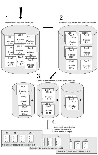
The MonetDB/XQUERY database system has the capability to create result pages with each result having a rank, title, snippet and URL. A number of steps had to be taken in order to create an environment where a number of search engines index disjoint (but not necessarily covering) subsets of the whole WT10g document collection. Each of these steps will be explained in the next subsection.
4.1.1 Creating Subcollections and their Result Pages
The MonetDB/XQUERY retrieval platform requires its data to be valid XML. Thus, the first step was to convert all WT10g data into valid XML. Therefore, a script was used that: 1) discarded the HTML comments, scripts, and all but the title and anchor HTML-tags; 2) truncated URLs ending in “/index....” at the index-portion; 3) glued consecutive sentences shorter than 20 characters together and split sentences longer than 160
1 A pool of documents is created from the top N documents submitted by TREC participants.
characters; finally, 4) in the case that a document did not have a title, a title was created from the first sentence of the document.
The documents (web pages) in the original WT10g corpus were randomly distributed over several file chunks. It is assumed that the pages of a website are highly related to each other and that they most often reside on the same web server. This led to the second step of re-grouping the documents by their IP-address, which resulted in XML-documents containing all web pages of a single server. We will refer to these newly created documents as ip-split documents.
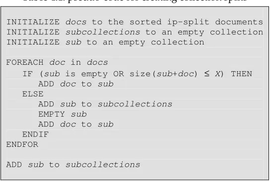
The third step is to create subcollections from these ip-split documents. A simple set of rules was used to create these subcollections. First, the ip-split documents were sorted by their file size. Then, each ip-split document ipdoc was added to a subcollection if the
combined size would not exceed a specified size of X MB. Otherwise, a new
subcollection was made containing ipdoc. Note that an ip-split document bigger than X
[image:28.595.162.435.336.519.2]MB was not split. In pseudo-code:
Table 4.1: pseudo-code for creating collection splits
INITIALIZE docs to the sorted ip-split documents INITIALIZE subcollections to an empty collection INITIALIZE sub to an empty collection
FOREACH doc in docs
IF (sub is empty OR size(sub+doc) ≤ X) THEN ADD doc to sub
ELSE
ADD sub to subcollections
EMPTY sub
ADD doc to sub
ENDIF ENDFOR
ADD sub to subcollections
A number of subcollections were made based on a 100MB and 500MB split. Splitting the WT10g collections in chunks of roughly 100MB resulted in 79 subcollections. Similarly, splitting in chunks of 500MB resulted in 15 subcollections.
The fourth and final step indexes each subcollection by a (separate) search engine, and queries the search engine to get the result lists (with a maximum of 50 results) needed for the result merging experiments.
The MonetDB/XQUERY database system was used to make separate indices for each subcollection. In addition, each query was issued twice; first using the OKAPI BM25 IR-model, and then using the Normalized Log-Likelihood Ratio (NLLR) IR-model.
Figure 4.1: simulating the creation of result pages in a distributed environment
Summarizing, after performing all these steps, the following data sets were created:
• 79 subcollections (of +/- 100MB), each subcollection containing:
o 100 different result pages created with the OKAPI IR-model
o 100 different result pages created with the NLLR IR-model
• 15 subcollections (of +/- 500MB), each subcollection containing:
o 100 different result pages created with the OKAPI IR-model
4.1.2 Selection Policies
When doing result merging, it is not the intention to merge all the results from all search
engines; otherwise, one could as well have used a centralized index1. This means that a
selection must be made about which search engines to use for merging. The selection can affect the results of the merging experiments; it is very likely that a random selection and one based on the best performing search engines for a particular query would yield significantly different merging results.
This raises the question for a suitable measure of a search engine’s performance. Let us pay closer attention to the well-known Average Precision (AP) measure [41]. For a given query, the equation for the AP of a ranked result list is:
AP =
documents
relevant
of
number
rank
R
rank
P
N
rank
∑
=
•
1
)
(
)
(
where N is the number of retrieved results, P(x) gives the precision2 at rank x, and the binary function R(x) is 1 if the result at rank x is relevant or 0 otherwise. The AP can take as output values any value between zero and one. The Mean Average Precision (MAP) is obtained by averaging over multiple queries’ AP.
[image:30.595.183.420.447.606.2]
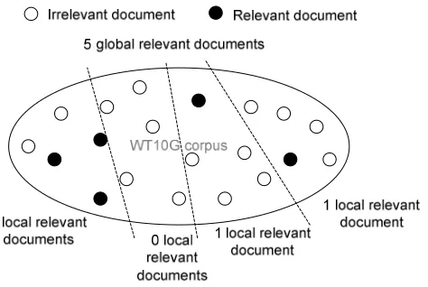
The WT10g relevance judgments contain a list of relevant documents per query; call these the global relevant documents. The WT10g collection is divided into several subcollections and we will refer to the number of relevant documents in such a collection as the local relevant documents. Figure 4.2 gives a simple example.
Figure 4.2: global versus local relevant documents.
Thus, for a given subcollection, the AP measure can be calculated by using either the global or the local relevant documents. The terms LAP, GAP, LMAP, and GMAP will be used to refer to local or global AP or MAP.
1 Under the following assumptions: first, a centralized IR system should perform at least as
good as a Distributed IR (DIR) system, since it has complete knowledge of the collection. Second, many search engines in a DIR environment contribute no relevant results.
2 The precision is defined as the number of relevant documents retrieved (at rank x), divided
Other ways of selecting search engines are random selection and selection based on the
engine’s merit, the number of relevant documents it contains. Keep in mind that these are
not performance measures.
4.2 SVM Models for Result Merging
An SVM model is affected by its training data and by its parameters. Sections 4.2.1 up to 4.2.4 explain how the results were converted to training data. Section 4.2.5 explains which parts of this data were actually used for training the SVM models, and how the parameters were varied.
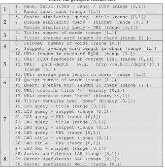
4.2.1 Features
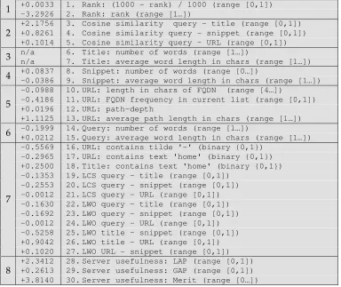
[image:31.595.132.467.329.670.2]SVM models are trained with labeled feature-vectors; these were extracted from the result lists for each query. Table 4.2 lists the thirty features used in our experiments; the range of each feature-value is given in the parenthesis at the end of the line.
Table 4.2: grouped feature list
1. Rank: ratio (1000 - rank) / 1000 (range [0,1])
1 2. Rank: local rank (range [1…])
3. Cosine similarity query - title (range [0,1]) 4. Cosine similarity query - snippet (range [0,1])
2
5. Cosine similarity query - URL (range [0,1]) 6. Title: number of words (range [1…])
3 7. Title: average word length in chars (range [1…])
8. Snippet: number of words (range [0…])
4 9. Snippet: average word length in chars (range [1…])
10.URL: length in chars of FQDN (range [4…])
11.URL: FQDN frequency in current list (range [0,1]) 12.URL: path-depth (e.g. http://a.b.c./depth=1/…)
(range [0…])
5
13.URL: average path length in chars (range [1…]) 14.Query: number of words (range [1…])
6 15.Query: average word length in chars (range [1…])
16.URL: contains tilde '~' (binary {0,1}) 17.URL: contains text 'home' (binary {0,1}) 18.Title: contains text 'home' (binary {0,1}) 19.LCS query - title (range [0,1])
20.LCS query - snippet (range [0,1]) 21.LCS query - URL (range [0,1]) 22.LWO query - title (range [0,1]) 23.LWO query - snippet (range [0,1]) 24.LWO query - URL (range [0,1]) 25.LWO title - snippet (range [0,1]) 26.LWO title - URL (range [0,1])
7
27.LWO URL - snippet (range [0,1]) 28.Server usefulness: LAP (range [0,1]) 29.Server usefulness: GAP (range [0,1])
8
30.Server usefulness: Merit (range [0…])
LCS(A,B) detects the biggest unaltered proportion of A that also appears exactly the same way in B. LWO(A,B) is almost similar to LCS, but it allows for noise. For example,
let A denote the text “using ranking SVM in IR” and let B denote “using Machine Learning
techniques for ranking in IR”. The LCS similarity between A and B is low (0.4), while we would expect otherwise. The LWO similarity does capture this apparent resemblance of A and B, yielding an LWO of 0.8. The pseudo code for LCS and LWO can be found in the Appendix A and B. The last three features are intended as a simple measure of the coherence of a result; do the title, snippet, and URL somewhat resemble each other?
Having extracted the feature vectors, we can now label them. A label is simply a digit and is placed at the start of each feature-vector. First, the concept of preference pair constraints will be explained, and then the appropriate labelings will be discussed for both the preference-SVM and regression-SVM.
4.2.2 Preference Pair Constraints
[image:32.595.148.449.369.535.2]Clickthrough data is a cheap source of relative relevance judgments and is used to create preference pair constraints. These constraints are used for training an SVM model (which should optimize the rankings of a search engine). Consider the result list in Table 4.3.
Table 4.3: example result list
1. Cattery Lopend Vuur
http://www.xs4all.nl/~bengaal 2. Supreme Show "Club Row" Stands
http://www.cityscape.co.uk/users/ja49/supclub.html 3. Tejas Bengal Cats
http://www.io.com/~tejas 4. Tejas Cattery
http://www.io.com/~tejas/whatis.htm 5. Nerd World : CATS
http://search.nerdworld.com/nw460.html
Suppose we are using clickthrough data and that a user actually clicked on results 1, 3, and 5. Joachims [18] argues that it is not possible to infer that results 1, 3, and 5 are relevant on an absolute scale; however, it is plausible to infer that result 3 is more relevant than result 2 with a probability higher than random. Assuming that the user scanned the ranking from top to bottom, he must have observed result 2 before clicking on 3, making a decision not to click on it. In other words, the search engine should have ranked result 3 higher than 2, and result 5 higher than 2 and 4. Denoting the ranking preferred by the user with r*, we get the following (partial and potentially noisy) preference constraints:
result3 <r* result2 result5 <r* result2 (4.1)
result5 <r* result4
and is based on superficial information supplied by the search engine (for example, ranks, titles, snippets, and URLs). Even if a result is judged more relevant (because a user clicked on it, but not on a higher ranked result), it does not mean than the result is
actually relevant. TREC judgments are absolute; a team of people have actually read the
entire document and rated that document as being irrelevant, relevant, or highly relevant. This brings us to the second difference: clickthrough data is “binary” (a result is either clicked on, or not) whereas TREC judgments are ternary.
Using TREC relevance judgments, consider again the result list in Table 4.3, where results 1, 3, and 5 are relevant, and where result 4 is highly relevant. The search engine should have ranked those results as follows: 4, 1, 3, 5, 2. The constraints are:
result3 <r* result2 result5 <r* result2 result4 <r* result1 (4.2) result4 <r* result2
result4 <r* result3
A final note on the use of preference pairs: Joachims states that for each clicked result, he adds fifty additional constraints indicating that it should be ranked higher than a random other result in the result set. The rationale is that those constraints should hold for the optimal ranking in most cases and they should both stabilize the learning result and keep the learned ranking function close to the original ranking function.
His result set consisted of 500 results. Since our result set consists of only 250 results, we used thirty instead of fifty additional constraints.
4.2.3 Preference-SVM Labeling
SVMlight automatically creates the constraints based on the labels of the training data. An
additional feature ‘qid’ is used to restrict the generation of the constraints; SVMlight
considers any two instances for a preference pair constraint only if they have equal ‘qid’ values. Such preference pairs are interpreted as follows: the instance with a higher label value should be ranked higher than the other one. For example: we could extract the feature-vectors from the results of Table 4.3, and label them as follows:
0 qid:1 (feature-vector for result 2) 1 qid:1 (feature-vector for result 3) 0 qid:2 (feature-vector for result 1) 0 qid:2 (feature-vector for result 2) 0 qid:2 (feature-vector for result 3) 1 qid:2 (feature-vector for result 4) 0 qid:3 (feature-vector for result 2) 1 qid:3 (feature-vector for result 5)
In the example, we see four instances having a ‘qid’ of two. If we create all possible pairs from these four instances, then those pairs with unequal labels are the preference constraints. Verify for yourself that the appropriate constraints (4.2) can be created based on the labels in the example above.
4.2.4 Regression-SVM Labeling
With regression-SVM, we aim to train a model that, given a feature-vector, will output a global (artificial) rank. We want this rank to reflect the knowledge obtained from both the TREC relevance judgments and from the rankings of the search engines. However, the TREC judgments should have a higher impact on the learned ranking function. For instance, if a highly relevant result (according to the TREC judgment) was ranked lowest by some search engine, then we certainly want our new ranking function to rank that result somewhere near the top.
From irrelevant to highly relevant, we denote the TREC judgments as 1, 2, and 3. We created the labels of the training instances by multiplying the instance’s relevance judgment by 1000, and then deducting its rank. This label, a global artificial rank, reflects the knowledge obtained from the TREC judgments and from the rankings of the search engines, while ensuring that the TREC judgments have a higher impact.
4.2.5 Model Settings
Preliminaries: Data Preparation & Feature Selection
Our training data consists of a subset of the results that were created in Section 4.1. Several subsets, or data chunks, could be used for training, for example, we could use the results of one search engine, or of three, or all, as our training data.
We used the result pages from the 100MB or the 500MB collection splits, indexed with either the NLLR or the OKAPI IR-models. We trained on the results of 1, 4, 7, 10 or 15 search engines, and we used the following policies to select the search engines: LAP, GAP, random, and merit.
When training on data from more than one search engine, we first applied a RR merge. Unfortunately, as the amount of training samples increased, so did the time required to train the SVM models. Therefore, we decided to merge no more than 250 results in a RR-fashion. Due to the large amount of time needed for training SVM models, we did not experiment with all the possible combinations using the OKAPI IR-model.
We divided our thirty features into eight feature groups (see the feature list, Table 4.2). Since we could not be certain whether some feature actually introduced noise or not, we did a simple feature selection experiment. In this experiment, we repeatedly trained a model while only changing one of the feature groups. That is, for each data chunk, we trained both a regression- and a preference-SVM model using either: all feature groups, or, each combination of seven out of all eight groups. A linear kernel was used in these preliminary experiments.
The preliminary experiments give an indication of the optimal data settings for learning a good SVM model, that is, they roughly indicate which data chunks and feature groups are best for either regression or preference SVM learning. Part of these results is shown in Chapter 5, Section 5.1.
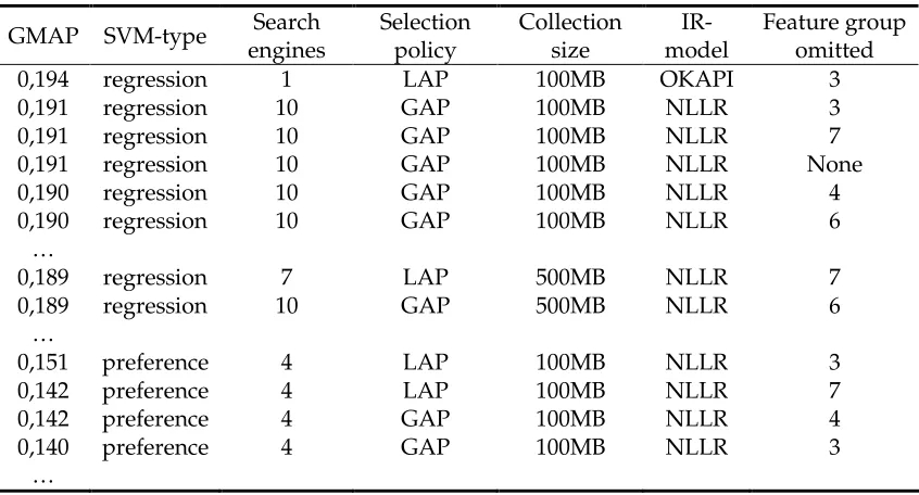
At first, we wanted to optimize the SVM parameters for the top three data settings, which are listed below:
• Regression: 100MB, OKAPI, 1 search engine, LAP, all features except group 3
• Regression: 100MB, NLLR, 10 search engines, GAP, all features except group 3
However, since there is only data from the 100MB split and since only regression models seem to perform best, we decided to use the following additional data settings, the best 500MB data setting and the two best settings for the preference-SVM:
• Regression: 500MB, NLLR, 7 search engines, LAP, all features except group 7
• Preference: 100MB, NLLR, 4 search engines, LAP, all features except group 3
• Preference: 100MB, NLLR, 4 search engines, LAP, all features except group 7
SVM Parameter Optimization
One parameter, which always applies, is the complexity factor C. This determines the trade-off between minimizing model error on the training data and minimizing model complexity. Its purpose is to avoid overfitting and underfitting. Overfitting occurs when the model performs well on the training data but does poorly on held-aside test data. Underfitting occurs when the model performs poorly on both training and test data. Another parameter is the kernel. Depending on the type of kernel used, additional kernel parameters must be specified1. Finally, in case SVM regression is used, an additional parameter epsilon must be specified; its purpose is to penalize large errors and neglect small ones.
For our experiments, we varied the C parameter from two to the power of 2.5, 2, 1.75,
-1.5, -1, 3, and 6. We used both a linear kernel and a Radial Basis Function (RBF) kernel. The gamma parameter for the RBF kernel was varied from four to the power of -1, 0, 1, 2, and 3. Finally, in the case of training regression models, the epsilon parameter was varied from five to the power of 0.5, 1, 1.5, 2, and 2.5.
Summarizing, the preliminary tests concluded that four data chunks were suitable for training regression models: for each chunk, we supplied 210 different parameter-combinations to the SVM algorithm. This resulted in 210 regression models: 35 with a linear kernel and 165 models with an RBF kernel. For each of the other two data chunks, we created 42 preference models: seven with a linear kernel and thirty-five with an RBF kernel.
We do not expect all 924 (4 x 210 and 2 x 42) models to generalize well, and we will discuss the evaluation of the SVM models in Section 4.4.1.
4.3 External Influences
We set out to analyze the effects of other variables, which we assumed to have great influence on the merging performance of our strategies.
4.3.1 Number of Result Lists
Merging more result lists inherently enhances recall. How this affects precision is hard to
say. For example, with RR merging, precision is very much affected by the quality of a
result list: it really matters that the first few results in each list are relevant. In many lists however, the first result is not relevant (that is, there are many lists of low quality) and no result list consists of only relevant results. Assuming that each time the list with the highest quality is selected next, then, as more result lists are being merged, precision will most likely increase until some optimum is reached, and then start to decrease.
By varying the amount of lists to be merged from 2, 3, 4, 5, 7, 10 and 15, we measured the precision-stability of each merging algorithm.
4.3.2 Subcollection Size
As the size of the subcollections increases, the number of the subcollections decreases. This has one major impact: the subcollection’s collection statistics are directly affected, influencing the IR-model’s performance and thus influencing the quality of the result pages.
A minor effect is that, as the size of the subcollections increases, the proportion of documents included in the search increases when the number of result lists to merge stays the same. For example, when merging 15 result lists, we are searching 100% of the documents if we use our 500MB collection split consisting of 15 subcollections.
4.3.3 Search Engine Selection Policy
Section 4.1.2 explained that Local/Global (Mean) Average Precision can be used as performance-based selection policies. In addition, two non-performance-based selection policies were explained: random selection and merit-based selection. We measured the effects of these six selection policies on the merging performance.
4.4 Evaluation
4.4.1 Evaluating SVM Models
We want to find out which model is the most robust model: that is, the one that produces
the highest GMAP as often as possible regardless of external influences: the resource selection policy used, the amount of search engines merged, and the size of the search engine’s document collection.
First, we split the result pages from each search engine for each query in two parts: the results of the odd queries for training and the results of the even queries for testing. However, not all results of all odd queries were used for training and not all results of all even queries were used for testing; instead, several data chunks were used. As discussed earlier in Section 4.2.5, six data chunks were selected: four chunks, each for training 210 regression models; and two chunks, each for training 42 preference models. The models were tr