Jian Feng
1, Lianyang Zou
1and Tianzhu Nan
21College of Computer Science and Technology, Xi’an University of Science and Technology, Xi’an, China 2Xi’an Fenghuo Software Technology Co., Ltd., Xi’an, China
A Phishing Webpage Detection Method
Based on Stacked Autoencoder and
Correlation Coefficients
Phishing is a kind of cyber-attack that targets naive online users by tricking them into revealing sensitive information. There are many anti-phishing solutions proposed to date, such as blacklist or whitelist, heuris-tic-based and machine learning-based methods. How-ever, online users are still being trapped into revealing sensitive information in phishing websites. In this pa-per, we propose a novel phishing webpage detection model, based on features that are extracted from URL, source codes of HTML, and the third-party services to represent the basic characters of phishing webpages, which uses a deep learning method – Stacked Auto-encoder (SAE) to detect phishing webpages. To make features in the same order of magnitude, three kinds of normalization methods are adopted. In particular, a method to calculate correlation coefficients between weight matrixes of SAE is proposed to determine opti-mal width of hidden layers, which shows high compu-tational efficiency and feasibility. Based on the testing of a set of phishing and benign webpages, the model using SAE achieves the best performance when com-pared to other algorithms such as Naive Bayes (NB), Support Vector Machine (SVM), Convolutional Neu-ral Networks (CNN), and Recurrent NeuNeu-ral Networks (RNN). It indicates that the proposed detection model is promising and can be applied effectively to phishing detection.
ACM CCS (2012) Classification: Security and privacy → Software and application security → Web applica-tion security
Keywords: phishing, deep learning, correlation coef-ficient
1. Introduction
Phishing refers to a kind of cyber-attack that uses social engineering, technical camouflage and other means of attack methods, by send-ing fraudulent spam, real-time communication messages, etc., to trick users into clicking on fake phishing pages, in order to entice users to disclose sensitive information such as personal-ly identifiable data and financial accounts. The Anti-Phishing Working Group (APWG) reports that the total number of phishing attacks in the first quarter of 2018 is a 46% increase over the last quarter of 2017 [1]. The continued growth of phishing attacks has had a huge negative im-pact on the healthy development of the Internet and has become one of the most serious securi-ty threats on the Internet.
Researchers have proposed a series of de-tection methods for phishing webpage, in-cluding blacklist-based detection methods, heuristic-based detection methods, visual sim-ilarity-based detection methods, and machine learning-based detection methods. Among them, machine learning-based detection meth-ods have achieved good detection results. How-ever, with speeding up of phishing webpage up-date and increasing of the complexity of feature data, traditional phishing detection technology still needs continuous improvement.
order to better detect phishing pages, a novel detection model for phishing webpages based on deep learning is proposed in this paper. Af-ter summarizing the existing research results, a detection model for phishing webpages is pro-posed. The model extracts the significant fea-tures of phishing webpages based on analyzing a large number of the latest phishing samples, and proposes a deep learning-based method that combines Stacked Autoencoder (SAE) with Softmax by a combination of unsupervised and supervised learning modes. Hence, in training of model parameters, a method for determining the width of hidden layers based on correlation coefficient is proposed, which effectively im-proves the training efficiency.
The main contributions in this paper are sum-marized as follows:
● To characterize phishing pages in all direc-tions and at multiple levels. Based on the analysis of phishing webpages, construct-ing 52-dimensional feature vectors for phishing webpage detection from struc-tural and lexical features of URL, Whois and DNS information, and source codes of HTML.
● To construct a phishing webpage detection model SSM (SAE-Softmax model), which is based on SAE and uses Softmax regres-sion model to make the classification. ● To determine the width of hidden layers
by correlation calculation between weight matrices of SAE, so that the width of hid-den layers can be effectively adjusted. The remaining sections of this paper are orga-nized as follows: Section II shows the related works. Background work for Autoencoder (AE) is shown in Section III. Section IV shows the implementation of SSM. Section V describes the datasets and the comparative experiments. Finally, Section VI draws the conclusion and provides some implications for future work on phishing detection.
2. Related Works
2.1. Traditional Detection Methods
At present, the mainstream phishing webpage detection methods mainly include four catego-ries.
1. Backlist-based detection methods simply
match information such as URLs, which are easily implemented and have no false positives, but cannot identify phishing pag-es which are not listed on the blacklist [2].
2. Heuristic-based detection methods
de-sign and implement heuristic rules based on the similarity between phishing pages. Typical detection systems include CAN-TINA+ [3], etc. These methods can detect most unreported phishing websites in real time, but the premise is that the statistical features of phishing pages are unique and fuzzy matching technologies are adopted, so the false positive rate is high.
3. Visual similarity-based detection
meth-ods convert the webpages to be detected into pictures and then compare the fea-ture vectors of the tested webpage and the targeting webpage by image processing technologies. A typical method is EMD al-gorithm proposed in [4]. This type of tech-nology is powerless for phishing webpages which are not visually similar to the target-ing webpage.
4. Machine learning-based detection
meth-ods treat the phishing webpage detection as classification or clustering problem and then use the corresponding machine learn-ing algorithms to construct the detection models. The clustering method first divides the webpage dataset into several clusters, and then distinguishes the phishing web-pages and the normal webweb-pages by marking the clusters [5]. The classification method constructs classification rules or classifiers based on the features of the labeled web-pages and then maps unknown webweb-pages to one of the given categories [6]. Although machine learning-based methods have good adaptability and extensibility, and the detection accuracy is high, tradition-al machine learning methods are shtradition-allow level algorithms, and the ability to express complex functions is limited in the case of finite samples and computational units. The generalization ability of complex clas-sification problems is limited.
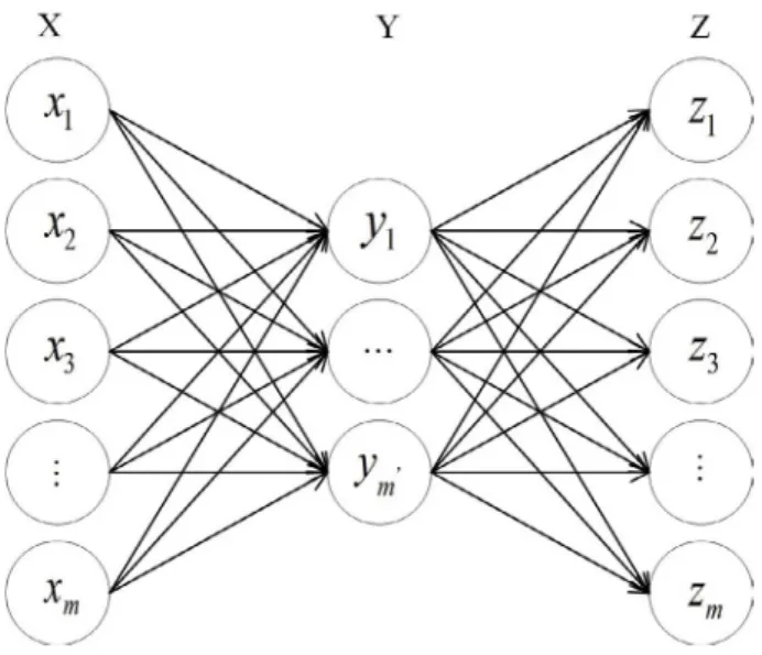
Considering a dataset X with n samples and m features, the output of encoder Y represents the reduced representation of X and the decoder is tuned to reconstruct the original X to Z from the encoder's representation Y by minimizing the difference between X and Z, as illustrated in Figure 1. Y is the real outcome, which rep-resents potential structure and characteristics of X. Specifically, the encoder is a function f that maps X to its hidden representation Y.
Figure 1. Diagram of the autoencoder.
The process is formulated as:
Y f X= ( )=S WX bf( + X) (1)
where Sf is a nonlinear activation function and
if it is an identity function, AE will do linear projection. The encoder is parameterized by a weight matrix W and a bias vector bX ∈ Rn.
The decoder function g maps hidden represen-tation Y back to a reconstruction Z:
Z g Y= ( )=S W'X bg( + Y) (2) where Sg is activation function of the decoder,
typically either the identity (yielding linear re-construction) or a sigmoid. The decoder's pa-rameters are biased vector bY and weight ma-trix W', where W' is the inverse matrix of W. In this paper, we only explore the case of the tied weights when W'=W T.
Training an AE involves finding parameters ( ,W b bX, )Y
θ = that minimize the reconstruc-2.2. Deep Learning-Based Methods
In 2006, Hinton et al. proposed deep learning theory and then several deep learning models such as Deep Belief Network (DBN), AE, Con-volutional Neural Networks (CNN), and Recur-rent Neural Networks (RNN) were proposed. It has demonstrated state of the art performance in many applications such as speech recogni-tion, natural language processing, etc. In recent years, researchers have applied deep learning to phishing webpage detection. For example, the literature [7-9] mentions applications of deep learning to analyze URLs, and the difference is that they use different methods, namely RNN, Denoising Autoencoder (DAE) and CNN, re-spectively. Instead of manually extracting the features, all these researches learned represen-tations from URL in different ways. On the other hand, there are some researches which focus on the texts on webpages and try to use new methods to learn new features represents phishing webpages. For example, in [10], fea-tures were extracted for phishing and benign webpages and classified using a Deep Belief Network-based detection model, while in [10], a series of semantic features were extracted through word2vec and used to describe the fea-tures of phishing webpages. Although all these solutions could classify the phishing websites precisely, they fail to use traditional phishing characters sufficiently. Following these suc-cesses, we propose a new model based on deep learning to solve the problem of webpage phish-ing detection by SAE and manually extracted statistical features, such as known stealing in-formation and third-party services.
3. Background
3.1. AE
order to better detect phishing pages, a novel detection model for phishing webpages based on deep learning is proposed in this paper. Af-ter summarizing the existing research results, a detection model for phishing webpages is pro-posed. The model extracts the significant fea-tures of phishing webpages based on analyzing a large number of the latest phishing samples, and proposes a deep learning-based method that combines Stacked Autoencoder (SAE) with Softmax by a combination of unsupervised and supervised learning modes. Hence, in training of model parameters, a method for determining the width of hidden layers based on correlation coefficient is proposed, which effectively im-proves the training efficiency.
The main contributions in this paper are sum-marized as follows:
● To characterize phishing pages in all direc-tions and at multiple levels. Based on the analysis of phishing webpages, construct-ing 52-dimensional feature vectors for phishing webpage detection from struc-tural and lexical features of URL, Whois and DNS information, and source codes of HTML.
● To construct a phishing webpage detection model SSM (SAE-Softmax model), which is based on SAE and uses Softmax regres-sion model to make the classification. ● To determine the width of hidden layers
by correlation calculation between weight matrices of SAE, so that the width of hid-den layers can be effectively adjusted. The remaining sections of this paper are orga-nized as follows: Section II shows the related works. Background work for Autoencoder (AE) is shown in Section III. Section IV shows the implementation of SSM. Section V describes the datasets and the comparative experiments. Finally, Section VI draws the conclusion and provides some implications for future work on phishing detection.
2. Related Works
2.1. Traditional Detection Methods
At present, the mainstream phishing webpage detection methods mainly include four catego-ries.
1. Backlist-based detection methods simply
match information such as URLs, which are easily implemented and have no false positives, but cannot identify phishing pag-es which are not listed on the blacklist [2].
2. Heuristic-based detection methods
de-sign and implement heuristic rules based on the similarity between phishing pages. Typical detection systems include CAN-TINA+ [3], etc. These methods can detect most unreported phishing websites in real time, but the premise is that the statistical features of phishing pages are unique and fuzzy matching technologies are adopted, so the false positive rate is high.
3. Visual similarity-based detection
meth-ods convert the webpages to be detected into pictures and then compare the fea-ture vectors of the tested webpage and the targeting webpage by image processing technologies. A typical method is EMD al-gorithm proposed in [4]. This type of tech-nology is powerless for phishing webpages which are not visually similar to the target-ing webpage.
4. Machine learning-based detection
meth-ods treat the phishing webpage detection as classification or clustering problem and then use the corresponding machine learn-ing algorithms to construct the detection models. The clustering method first divides the webpage dataset into several clusters, and then distinguishes the phishing web-pages and the normal webweb-pages by marking the clusters [5]. The classification method constructs classification rules or classifiers based on the features of the labeled web-pages and then maps unknown webweb-pages to one of the given categories [6]. Although machine learning-based methods have good adaptability and extensibility, and the detection accuracy is high, tradition-al machine learning methods are shtradition-allow level algorithms, and the ability to express complex functions is limited in the case of finite samples and computational units. The generalization ability of complex clas-sification problems is limited.
Considering a dataset X with n samples and m features, the output of encoder Y represents the reduced representation of X and the decoder is tuned to reconstruct the original X to Z from the encoder's representation Y by minimizing the difference between X and Z, as illustrated in Figure 1. Y is the real outcome, which rep-resents potential structure and characteristics of X. Specifically, the encoder is a function f that maps X to its hidden representation Y.
Figure 1. Diagram of the autoencoder.
The process is formulated as:
Y f X= ( )=S WX bf( + X) (1)
where Sf is a nonlinear activation function and
if it is an identity function, AE will do linear projection. The encoder is parameterized by a weight matrix W and a bias vector bX ∈ Rn.
The decoder function g maps hidden represen-tation Y back to a reconstruction Z:
Z g Y= ( )=S W'X bg( + Y) (2) where Sg is activation function of the decoder,
typically either the identity (yielding linear re-construction) or a sigmoid. The decoder's pa-rameters are biased vector bY and weight ma-trix W', where W' is the inverse matrix of W. In this paper, we only explore the case of the tied weights when W'=W T.
Training an AE involves finding parameters ( ,W b bX, )Y
θ = that minimize the reconstruc-2.2. Deep Learning-Based Methods
In 2006, Hinton et al. proposed deep learning theory and then several deep learning models such as Deep Belief Network (DBN), AE, Con-volutional Neural Networks (CNN), and Recur-rent Neural Networks (RNN) were proposed. It has demonstrated state of the art performance in many applications such as speech recogni-tion, natural language processing, etc. In recent years, researchers have applied deep learning to phishing webpage detection. For example, the literature [7-9] mentions applications of deep learning to analyze URLs, and the difference is that they use different methods, namely RNN, Denoising Autoencoder (DAE) and CNN, re-spectively. Instead of manually extracting the features, all these researches learned represen-tations from URL in different ways. On the other hand, there are some researches which focus on the texts on webpages and try to use new methods to learn new features represents phishing webpages. For example, in [10], fea-tures were extracted for phishing and benign webpages and classified using a Deep Belief Network-based detection model, while in [10], a series of semantic features were extracted through word2vec and used to describe the fea-tures of phishing webpages. Although all these solutions could classify the phishing websites precisely, they fail to use traditional phishing characters sufficiently. Following these suc-cesses, we propose a new model based on deep learning to solve the problem of webpage phish-ing detection by SAE and manually extracted statistical features, such as known stealing in-formation and third-party services.
3. Background
3.1. AE
tion loss on X and Z, the objective function is given as:
θ =min ( , ) min ( , ( ( )))θ L X Z = θ L X g f X . (3) For linear reconstruction, the reconstruction loss (L1) is generally calculated by the squared
error:
2 2
1
1 1
( ) n i i n i ( ( ))i
i i
L θ x z x g f x
= =
=
∑
− =∑
− (4)For nonlinear reconstruction, the reconstruction loss (L2) is generally from cross-entropy:
[
]
2
1
( ) n ilog( ) (1i i)log(1 i)
i
L θ x y x y
=
= −
∑
+ − − (5)where xi∈ X, zi∈ Z and yi∈ Y.
In SAE, the weight matrix W and the offset b are adjusted layer-by-layer by stochastic gradi-ent descgradi-ent:
W ←W−η ∂L X Z( , )∂W (6)
b← −b η ∂L X Z( , )b
∂ (7)
where η is the learning rate.
3.2. SAE
AE contains only one hidden layer, which is a shallow learning model. The limitation of the shallow learning model is that the ability to rep-resent complex functions is limited in the case of finite samples and computational units, and its generalization ability is constrained for com-plex problems. A major advantage of AE is that it is easy to be stacked for generating different
levels of new features to represent original ones by adding hidden layers. After training to get the first AE, take its hidden layer as input, use the same method to train the second AE, and then train to get multiple AEs. Multiple AEs are stacked together to form an SAE model. The training process of SAE is shown in Figure 2. For an SAE with totally H hidden layers, the process of encoding is:
Y f= H(⋅⋅⋅ ⋅⋅⋅fi( f X1( ))) (8)
where fi is the encoding function of layer i. The
corresponding decoding function is:
Z g= H(⋅⋅⋅ ⋅⋅⋅gi( g Y1( ))) (9) where gi is the decoding function of layer i and
the SAE can be trained by a greedy layer-wise feed-forward approach.
Finally, SAE is combined with Softmax to construct SSM model. The features learned by SAE are used as input to the Softmax classifier to obtain the final classification result.
4. Proposed Methodology
4.1. Problem Setting and Systematic Design
Our goal is to classify a given webpage as ma-licious or not. We do this by formulating the problem as a binary classification task. Consid-er a set of N webpages, {(P1, L1), ..., (Pi, Li),
..., (PN, LN)}, where i = 1, ..., N, Pi represents a
webpage, and Ci ∈{-1, +1} denotes the label
of the webpage, with Ci = +1 being a malicious
webpage, and Ci = -1 being a benign webpage.
The first step in the classification procedure is to obtain a feature representation Pi → xi where
xi∈Rm is the m-dimensional feature vector
rep-resenting webpage PN. The next step is to learn
a prediction function f : Rm → R to predict the
score of the class assignment for a webpage in-stance. The prediction made by f is denoted as
( ( ))
Z sign f p= . The aim is to learn a function that can minimize the total number of mistakes in the entire dataset. This is often achieved by minimizing a loss function. In our methodol-ogy, the function f is represented as an SAE network, and the cross-entropy loss function is adopted.
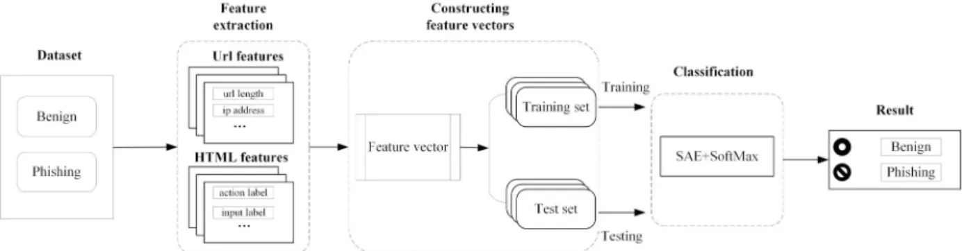
The systematic design of the SSM is illustrated in Figure 3. The input comprises a set of benign webpages and phishing webpages. Selection of features and normalization processes are car-ried out in the feature extraction phase. Then the SAE network is used to implement data reconstruction, and Softmax is added as a su-pervised classifier to assist in adjusting the net-work, and then binary classification of benign and phishing webpages is carried out.
4.2. Feature Extraction
The first step of obtaining feature representation deals with obtaining useful information from URL and webpage that can be stored in a vector so that the methods based on machine learning can be applied to it. Various types of features have been considered. We have classified the extracted features into two categories includ-ing URL related features and HTML based features. There is a total of 52 features which form a vector of 52 dimensions for a webpage Pi, namely xi = x xi0, , ...,1i xi51 .
4.2.1. URL Related Features
URL related features are divided into URL-based features and third-party service features, and the third-party service features further include DNS-based features, Whois-based features, and ranking features.
● URL-based features
Table 1 lists some of the typical features ex-tracted from URLs.
Table 1. URL-based features.
Feature Type Description
Length Numeric Length of a URL IP address Bool Whether there is IP address in URL
Depth Numeric Number of '/' in URL @ Bool Whether there is @ in URL ● DNS-based features
Table 2 lists some of the typical features ex-tracted from DNS information corresponding to the domain in URLs.
Table 2. DNS-based features.
Feature Type Description
Missing
information Bool Whether there is information missing in DNS A record Numeric Number of A records in DNS NS record Numeric Number of NS records in DNS ● Whois-based features
Whois describes the details of the DNS, includ-ing whether the domain is registered, by whom it was registered, registrar, registration time, updated time, destruction time, and so on. Typ-ical features are shown in Table 3.
Table 3. Whois-based features.
Feature Type Description
Missing
information Bool Whether there is informa-tion missing in Whois End time Numeric current time and termina-The difference between tion time of the domain Survival
time Numeric
The difference between ter-mination time and creation
time of the domain
Figure 3. The architecture of SSM.
tion loss on X and Z, the objective function is given as:
θ =min ( , ) min ( , ( ( )))θ L X Z = θ L X g f X . (3) For linear reconstruction, the reconstruction loss (L1) is generally calculated by the squared
error:
2 2
1
1 1
( ) n i i n i ( ( ))i
i i
L θ x z x g f x
= =
=
∑
− =∑
− (4)For nonlinear reconstruction, the reconstruction loss (L2) is generally from cross-entropy:
[
]
2
1
( ) n ilog( ) (1i i)log(1 i)
i
L θ x y x y
=
= −
∑
+ − − (5)where xi∈ X, zi∈ Z and yi∈ Y.
In SAE, the weight matrix W and the offset b are adjusted layer-by-layer by stochastic gradi-ent descgradi-ent:
W ←W−η ∂L X Z( , )∂W (6)
b← −b η ∂L X Z( , )b
∂ (7)
where η is the learning rate.
3.2. SAE
AE contains only one hidden layer, which is a shallow learning model. The limitation of the shallow learning model is that the ability to rep-resent complex functions is limited in the case of finite samples and computational units, and its generalization ability is constrained for com-plex problems. A major advantage of AE is that it is easy to be stacked for generating different
levels of new features to represent original ones by adding hidden layers. After training to get the first AE, take its hidden layer as input, use the same method to train the second AE, and then train to get multiple AEs. Multiple AEs are stacked together to form an SAE model. The training process of SAE is shown in Figure 2. For an SAE with totally H hidden layers, the process of encoding is:
Y f= H(⋅⋅⋅ ⋅⋅⋅fi( f X1( ))) (8)
where fi is the encoding function of layer i. The
corresponding decoding function is:
Z g= H(⋅⋅⋅ ⋅⋅⋅gi( g Y1( ))) (9) where gi is the decoding function of layer i and
the SAE can be trained by a greedy layer-wise feed-forward approach.
Finally, SAE is combined with Softmax to construct SSM model. The features learned by SAE are used as input to the Softmax classifier to obtain the final classification result.
4. Proposed Methodology
4.1. Problem Setting and Systematic Design
Our goal is to classify a given webpage as ma-licious or not. We do this by formulating the problem as a binary classification task. Consid-er a set of N webpages, {(P1, L1), ..., (Pi, Li),
..., (PN, LN)}, where i = 1, ..., N, Pi represents a
webpage, and Ci ∈{-1, +1} denotes the label
of the webpage, with Ci = +1 being a malicious
webpage, and Ci = -1 being a benign webpage.
The first step in the classification procedure is to obtain a feature representation Pi → xi where
xi∈Rm is the m-dimensional feature vector
rep-resenting webpage PN. The next step is to learn
a prediction function f : Rm → R to predict the
score of the class assignment for a webpage in-stance. The prediction made by f is denoted as
( ( ))
Z sign f p= . The aim is to learn a function that can minimize the total number of mistakes in the entire dataset. This is often achieved by minimizing a loss function. In our methodol-ogy, the function f is represented as an SAE network, and the cross-entropy loss function is adopted.
The systematic design of the SSM is illustrated in Figure 3. The input comprises a set of benign webpages and phishing webpages. Selection of features and normalization processes are car-ried out in the feature extraction phase. Then the SAE network is used to implement data reconstruction, and Softmax is added as a su-pervised classifier to assist in adjusting the net-work, and then binary classification of benign and phishing webpages is carried out.
4.2. Feature Extraction
The first step of obtaining feature representation deals with obtaining useful information from URL and webpage that can be stored in a vector so that the methods based on machine learning can be applied to it. Various types of features have been considered. We have classified the extracted features into two categories includ-ing URL related features and HTML based features. There is a total of 52 features which form a vector of 52 dimensions for a webpage Pi, namely xi = x xi0, , ...,1i xi51 .
4.2.1. URL Related Features
URL related features are divided into URL-based features and third-party service features, and the third-party service features further include DNS-based features, Whois-based features, and ranking features.
● URL-based features
Table 1 lists some of the typical features ex-tracted from URLs.
Table 1. URL-based features.
Feature Type Description
Length Numeric Length of a URL IP address Bool Whether there is IP address in URL
Depth Numeric Number of '/' in URL @ Bool Whether there is @ in URL ● DNS-based features
Table 2 lists some of the typical features ex-tracted from DNS information corresponding to the domain in URLs.
Table 2. DNS-based features.
Feature Type Description
Missing
information Bool Whether there is information missing in DNS A record Numeric Number of A records in DNS NS record Numeric Number of NS records in DNS ● Whois-based features
Whois describes the details of the DNS, includ-ing whether the domain is registered, by whom it was registered, registrar, registration time, updated time, destruction time, and so on. Typ-ical features are shown in Table 3.
Table 3. Whois-based features.
Feature Type Description
Missing
information Bool Whether there is informa-tion missing in Whois End time Numeric current time and termina-The difference between tion time of the domain Survival
time Numeric
The difference between ter-mination time and creation
time of the domain
Figure 3. The architecture of SSM.
● Ranking features
The ranking features, shown in Table 4, are mainly based on the Alexa Rank, which is also known as the page level.
Table 4. Ranking features.
Feature Type Description
Ranking Numeric The comprehensive rank of webpages on Alexa Rank Visiting traffic
ranking Numeric Visiting rank on Alexa Rank
4.2.2. HTML-Based Features
This paper divides the HTML-based features into three categories. In order to calculate val-ues of the first two types of features, here are a few symbol definitions: L represents the num-ber of links in the attribute of current tag. LE represents the number of empty links in the at-tribute of current tag. LC represents the number of links pointing to the current domain in the attribute of current tag.
● Feature of empty links
To count the empty links in the attribute of tags, calculate ME:
0 if 0
/ if 0
1 Tag does not exist LE
ME LE L LE
=
= >
−
(10)
● Feature of pointing to the current domain To count the links to the current domain in the attribute of tags, calculate MC:
0 if 0
/ if 0
1 Tag does not exist LC
MC LC L LC
=
= >
−
(11)
● The third type of features, including the ti-tle attribute and the keyword attribute, is all Bool.
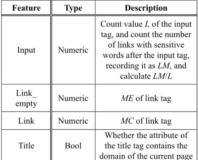
Table 5 lists some of the typical features ex-tracted from HTML.
4.3. Normalization
To make features in the same order of magni-tude, we made the value of the features nor-malized to [0, 1]. Assuming that the j-th feature xi,j of the sample xi is numeric, three kinds of
normalization algorithms are adopted, namely Minimum_Maximum normalization, Statisti-cal normalization, and Decimal normalization. Their respective formula is as follows:
● Minimum_Maximum normalization
, ,
1 ,
, ,
min( ) ( i j) max( ) min( )i j j
j j
x x
f x = x− x
− (12)
where min(x ,j) and max(x ,j) are minimum and
maximum values of the j-th attribute of all sam-ples, respectively.
● Statistical normalization
f x2( i j, ) (= xi j, −µ σ) / (13) where µ represents the average of the j-th attri-bute of all samples, and σ is the standard devi-ation.
● Decimal normalization
f x3( i j, )=xi j, /10q (14) where q is the smallest integer to enable the maximum of the j-th attribute is in the interval [0, 1].
4.4. Parameter Optimization of SSM
Experience has shown that the performance of deep learning models depends mainly on the network structure, especially the width of hid-den layers. However, the selection of the num-ber of hidden layer nodes is a very complicated problem. For the classification problem, if the width of hidden layers is too small, the training and testing accuracy will be relatively poor, and it is difficult to deal with complicated problems; if the width is too large, the training will take too long, and the classification performance will decrease, resulting in over-fitting. The methods for determining the width are mainly trial and error method [12], empirical formu-la method [13], growth method [14], pruning method [15], adaptive increase and decrease algorithm [16], genetic algorithm [17], etc. However, these methods have their limitations. The trial and error method is a kind of blindly searching algorithm with a large computation-al overhead. The empiriccomputation-al formula method is completely based on experience, as it lacks the corresponding theoretical basis. It is effective for specific samples but lacks a universal for-mula. Growth and pruning are the most studied methods at present. The growth method starts with the fewest number of nodes and then grad-ually adds new nodes until the network struc-ture is optimal, and the pruning rule does the same in reverse. However, when to terminate is a problem for both methods, so the calcula-tion costs of both algorithms are huge. Genetic algorithm is generally used in conjunction with the growth method or the pruning method. The main problem is that the convergence speed is slow and prone to oscillation.
In order to determine the suitable width of hid-den layers quickly, this paper proposes an adap-tive optimization algorithm based on weight correlation.
4.4.1. Basic Idea
According to the definition of the correlation coefficient, the absolute value of the correlation coefficient R between the two variables is be-tween 0 and 1. The closer |R| is to 0, the smaller the correlation between the two variables. Ac-cording to the theory of detection, R between the samples has a significant influence on the
error rate of the classification, and the best ef-fect of the classification is optimal when R is 0. SAE is a multi-layered network. If taking weights of the nodes in the hidden layer as sam-ples, then the closer the correlation coefficient between these weights is to 0, the larger the difference between the nodes, and perhaps the better the classification effect will be. Based on the above analysis, our goal is to find the net-work structure that maximizes the gap among the hidden layer nodes and select the width of hidden layers in this case.
This paper completes this process in two steps. The first is to initialize the network structure by setting the widths of the input layer and the first hidden layer. The number of input neurons equals the feature dimension of the input data, and the number of nodes in the first hidden lay-er is set artificially. Because we have not detlay-er- deter-mined the explicit relationship between the in-put dimension and the width in the first hidden layer, the width in the first hidden layer cannot be adjusted automatically, and therefore is only set to be less than the input neurons. The second step is to determine the width of other hidden layers. A method to calculate correlation coeffi-cient between weight matrices is proposed here, and it is used to determine the width of the cur-rent layer.
4.4.2. Determination of the Width by Correlation Coefficient
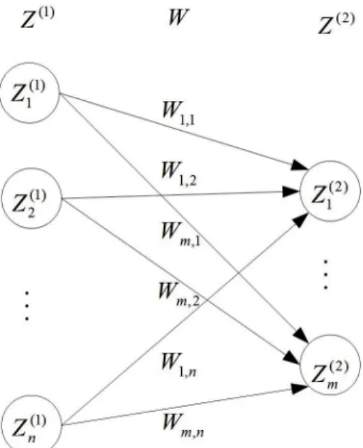
First, we clarify the concept of weight matrix. Weight matrix is a matrix formed by the con-nection weights among all nodes of the current layer and the previous layer.
For example, Figure 4 shows weights between two hidden layers. And its weights matrix is shown as W.
1,1 1, 2 1,
2,1 2, 2 2,
,1 , 2 ,
n n
m m m n
w w w
w w w
W
w w w
=
The elements in W, while i = 1, 2, ..., m, and j = 1, 2, ..., n, represent weight of the connection between the i-th neuron of the current layer and
Table 5. HTML-based features.
Feature Type Description
Input Numeric
Count value L of the input tag, and count the number
of links with sensitive words after the input tag,
recording it as LM, and calculate LM/L
Link_
empty Numeric ME of link tag Link Numeric MC of link tag Title Bool Whether the attribute of the title tag contains the
● Ranking features
The ranking features, shown in Table 4, are mainly based on the Alexa Rank, which is also known as the page level.
Table 4. Ranking features.
Feature Type Description
Ranking Numeric The comprehensive rank of webpages on Alexa Rank Visiting traffic
ranking Numeric Visiting rank on Alexa Rank
4.2.2. HTML-Based Features
This paper divides the HTML-based features into three categories. In order to calculate val-ues of the first two types of features, here are a few symbol definitions: L represents the num-ber of links in the attribute of current tag. LE represents the number of empty links in the at-tribute of current tag. LC represents the number of links pointing to the current domain in the attribute of current tag.
● Feature of empty links
To count the empty links in the attribute of tags, calculate ME:
0 if 0
/ if 0
1 Tag does not exist LE
ME LE L LE
=
= >
−
(10)
● Feature of pointing to the current domain To count the links to the current domain in the attribute of tags, calculate MC:
0 if 0
/ if 0
1 Tag does not exist LC
MC LC L LC
=
= >
−
(11)
● The third type of features, including the ti-tle attribute and the keyword attribute, is all Bool.
Table 5 lists some of the typical features ex-tracted from HTML.
4.3. Normalization
To make features in the same order of magni-tude, we made the value of the features nor-malized to [0, 1]. Assuming that the j-th feature xi,j of the sample xi is numeric, three kinds of
normalization algorithms are adopted, namely Minimum_Maximum normalization, Statisti-cal normalization, and Decimal normalization. Their respective formula is as follows:
● Minimum_Maximum normalization
, ,
1 ,
, ,
min( ) ( i j) max( ) min( )i j j
j j
x x
f x = x− x
− (12)
where min(x ,j) and max(x ,j) are minimum and
maximum values of the j-th attribute of all sam-ples, respectively.
● Statistical normalization
f x2( i j, ) (= xi j, −µ σ) / (13) where µ represents the average of the j-th attri-bute of all samples, and σ is the standard devi-ation.
● Decimal normalization
f x3( i j, )=xi j, /10q (14) where q is the smallest integer to enable the maximum of the j-th attribute is in the interval [0, 1].
4.4. Parameter Optimization of SSM
Experience has shown that the performance of deep learning models depends mainly on the network structure, especially the width of hid-den layers. However, the selection of the num-ber of hidden layer nodes is a very complicated problem. For the classification problem, if the width of hidden layers is too small, the training and testing accuracy will be relatively poor, and it is difficult to deal with complicated problems; if the width is too large, the training will take too long, and the classification performance will decrease, resulting in over-fitting. The methods for determining the width are mainly trial and error method [12], empirical formu-la method [13], growth method [14], pruning method [15], adaptive increase and decrease algorithm [16], genetic algorithm [17], etc. However, these methods have their limitations. The trial and error method is a kind of blindly searching algorithm with a large computation-al overhead. The empiriccomputation-al formula method is completely based on experience, as it lacks the corresponding theoretical basis. It is effective for specific samples but lacks a universal for-mula. Growth and pruning are the most studied methods at present. The growth method starts with the fewest number of nodes and then grad-ually adds new nodes until the network struc-ture is optimal, and the pruning rule does the same in reverse. However, when to terminate is a problem for both methods, so the calcula-tion costs of both algorithms are huge. Genetic algorithm is generally used in conjunction with the growth method or the pruning method. The main problem is that the convergence speed is slow and prone to oscillation.
In order to determine the suitable width of hid-den layers quickly, this paper proposes an adap-tive optimization algorithm based on weight correlation.
4.4.1. Basic Idea
According to the definition of the correlation coefficient, the absolute value of the correlation coefficient R between the two variables is be-tween 0 and 1. The closer |R| is to 0, the smaller the correlation between the two variables. Ac-cording to the theory of detection, R between the samples has a significant influence on the
error rate of the classification, and the best ef-fect of the classification is optimal when R is 0. SAE is a multi-layered network. If taking weights of the nodes in the hidden layer as sam-ples, then the closer the correlation coefficient between these weights is to 0, the larger the difference between the nodes, and perhaps the better the classification effect will be. Based on the above analysis, our goal is to find the net-work structure that maximizes the gap among the hidden layer nodes and select the width of hidden layers in this case.
This paper completes this process in two steps. The first is to initialize the network structure by setting the widths of the input layer and the first hidden layer. The number of input neurons equals the feature dimension of the input data, and the number of nodes in the first hidden lay-er is set artificially. Because we have not detlay-er- deter-mined the explicit relationship between the in-put dimension and the width in the first hidden layer, the width in the first hidden layer cannot be adjusted automatically, and therefore is only set to be less than the input neurons. The second step is to determine the width of other hidden layers. A method to calculate correlation coeffi-cient between weight matrices is proposed here, and it is used to determine the width of the cur-rent layer.
4.4.2. Determination of the Width by Correlation Coefficient
First, we clarify the concept of weight matrix. Weight matrix is a matrix formed by the con-nection weights among all nodes of the current layer and the previous layer.
For example, Figure 4 shows weights between two hidden layers. And its weights matrix is shown as W.
1,1 1, 2 1,
2,1 2, 2 2,
,1 , 2 ,
n n
m m m n
w w w
w w w
W
w w w
=
The elements in W, while i = 1, 2, ..., m, and j = 1, 2, ..., n, represent weight of the connection between the i-th neuron of the current layer and
Table 5. HTML-based features.
Feature Type Description
Input Numeric
Count value L of the input tag, and count the number
of links with sensitive words after the input tag,
recording it as LM, and calculate LM/L
Link_
empty Numeric ME of link tag Link Numeric MC of link tag Title Bool Whether the attribute of the title tag contains the
the j-th neuron of the previous layer where m is the number of neurons in the current layer and n is the number of neurons in the previous layer.
When a hidden layer adopts different widths, the network structure will change, so the weight matrix W will change accordingly. We want to determine the optimal width by learning the correlation of these weight matrices.
Firstly, we need to get the weight matrices un-der different network structures. To do this, on the basis of the initial width, we increase the width of the current hidden layer by the fixed nodes (for example, t) each round, until the to-tal width is greater than or equal to the width of the previous layer. A weight matrix between the current hidden layer and the previously hidden layer will be got each round.
For example, assuming the width of the previ-ous layer is o, the width of the previprevi-ous round of the current layer is s, and the weight matrix is denoted as A; if the width of the current round of the current layer is s + t (s + t ≤ o), then the weight matrix is denoted as B.
1,1 1, 2 1,
2,1 2, 2 2,
,1 , 2 ,
o o
s s s o
wa wa wa
wa wa wa
A
wa wa wa
=
1,1 1, 2 1,
2,1 2, 2 2,
,1 , 2 ,
o o
s t s t s t o
wb wb wb
wb wb wb
B
wb+ wb+ wb+
=
And then we try to perform correlation analysis on these matrices. Here a method for calculat-ing correlation coefficient between neighborcalculat-ing matrices is needed. Take correlation coefficient between A and B as example. Since s ≠ s + t, the correlation coefficient between A and B cannot be calculated directly through traditional meth-od. We first set the average of the values of the same column of each matrix to get two row vectors A' and B'. Where:
1, 2, ..., o
A'= wa wa wa
1, 2, ..., o ,
B'= wb wb wb
while:
1,j 2,j ... s j, ,
j
wa wa wa
wa = + s+ +
1,j 2,j ... s t j, , 1, 2, ..., .
j
wb wb wb
wb = + s t++ + + j= o
Then average all the elements of the two gener-ated row vectors to get two mean values:
1 2 ... o,
wa wa wa
wa= + o+ +
1 2 ... o.
wb wb wb
wb= + o+ +
Bring these values into classical correlation co-efficient equation to get the correlation coeffi-cient between the two matrices, see [15]:
(
)(
)
(
) (
)
1
2 2
1 1
o
j j
j
o o
j j
j j
wa wa wb wb R
wa wa wb wb
=
= =
− −
=
− −
∑
∑
∑
(15)
where R is correlation coefficient between
A and B. After all correlation coefficients for neighboring rounds are calculated, we set the width to the number of nodes whose absolute value of correlation coefficient is nearest to 0.
5. Experimental Results and Analysis
In order to verify the feasibility and effective-ness of SSM, we designed three sets of exper-iments.
5.1. Experimental Preparation
5.1.1. Experimental Environment
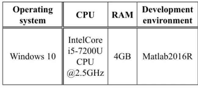
The experimental development environment is shown in Table 6. The fixed hyperparameters used in SSM are as follows: learning rate equals to 0.1, weight regularization is 0.001, times of iterations is 1000, activation function is ReLu, and loss function is cross-entropy. The hyper-parameters adjusted in experiments are the number of hidden layers and the width of the hidden layer.
Table 6. Development environment.
Operating
system CPU RAM Development environment
Windows 10
IntelCore i5-7200U
CPU @2.5GHz
4GB Matlab2016R
5.1.2. Basic Dataset
The basic dataset used in the experiments is ob-tained from the real network environment. The legal webpages come from Alexa. Alexa is a dedicated website managed by Amazon to pub-lish an authoritative ranking of websites, so it has a large number of URLs and detailed rank-ing information. After filterrank-ing out some inval-id, erroneous and duplicate pages, we collected 8,848 benign webpages from Alexa.
The phishing webpages are from PhishTank. com, which is an internationally renowned website that collects a timely and authoritative list of phishing webpages. We collected 11,321 phishing webpages listed on PhishTank from February 2016 to April 2016. In addition, web-pages that do not conform to grammar rules and benign webpages mixed in phishing datasets are processed.
We collected and saved URL, HTML source file, and a screenshot of each collected page.
5.1.3. Evaluating Indicators
The various evaluating indicators in literature were summarized, the most commonly used are Accuracy, Recall, True Positive Rate (TPR), False Positive Rate (FPR), True Negative Rate (TNR) and False Negative Rate (FNR), shown in Table 7.
Table 7. Evaluating indicators.
Evaluating indicators Formula
Accuracy (TP+TN) / (TP+TN+FP+FN) TPR (Recall) TP / (TP + FN)
FPR FP / (TN + FP) TNR TN / (TN + FP) FNR FN / (TP + FN)
In Table 7, TP (True Positive) denotes the num-ber of benign webpages correctly classified as benign webpages, FP (False Positive) denotes the number of phishing webpages classified as benign webpages, TN (True Negative) denotes the number of phishing webpages classified as phishing webpages, and FN (False Negative) denotes the number of benign webpages classi-fied as phishing webpages.
5.1.4. Baselines
In order to see how well the proposed SSM models perform with respect to the existing methods for phishing webpage detection, we compare SSM with four baseline models: Sup-port Vector Machines (SVM), Naive Bayes (NB), CNN and RNN.
5.2. Result Evaluation
5.2.1. Experiment 1: Determining the Number of Hidden Layers
This experiment aims to determine the optimal number of hidden layers in SAE. In the
the j-th neuron of the previous layer where m is the number of neurons in the current layer and n is the number of neurons in the previous layer.
When a hidden layer adopts different widths, the network structure will change, so the weight matrix W will change accordingly. We want to determine the optimal width by learning the correlation of these weight matrices.
Firstly, we need to get the weight matrices un-der different network structures. To do this, on the basis of the initial width, we increase the width of the current hidden layer by the fixed nodes (for example, t) each round, until the to-tal width is greater than or equal to the width of the previous layer. A weight matrix between the current hidden layer and the previously hidden layer will be got each round.
For example, assuming the width of the previ-ous layer is o, the width of the previprevi-ous round of the current layer is s, and the weight matrix is denoted as A; if the width of the current round of the current layer is s + t (s + t ≤ o), then the weight matrix is denoted as B.
1,1 1, 2 1,
2,1 2, 2 2,
,1 , 2 ,
o o
s s s o
wa wa wa
wa wa wa
A
wa wa wa
=
1,1 1, 2 1,
2,1 2, 2 2,
,1 , 2 ,
o o
s t s t s t o
wb wb wb
wb wb wb
B
wb+ wb+ wb+
=
And then we try to perform correlation analysis on these matrices. Here a method for calculat-ing correlation coefficient between neighborcalculat-ing matrices is needed. Take correlation coefficient between A and B as example. Since s ≠ s + t, the correlation coefficient between A and B cannot be calculated directly through traditional meth-od. We first set the average of the values of the same column of each matrix to get two row vectors A' and B'. Where:
1, 2, ..., o
A'= wa wa wa
1, 2, ..., o ,
B'= wb wb wb
while:
1,j 2,j ... s j, ,
j
wa wa wa
wa = + s+ +
1,j 2,j ... s t j, , 1, 2, ..., .
j
wb wb wb
wb = + s t++ + + j= o
Then average all the elements of the two gener-ated row vectors to get two mean values:
1 2 ... o,
wa wa wa
wa= + o+ +
1 2 ... o.
wb wb wb
wb= + o+ +
Bring these values into classical correlation co-efficient equation to get the correlation coeffi-cient between the two matrices, see [15]:
(
)(
)
(
) (
)
1
2 2
1 1
o
j j
j
o o
j j
j j
wa wa wb wb R
wa wa wb wb
=
= =
− −
=
− −
∑
∑
∑
(15)
where R is correlation coefficient between
A and B. After all correlation coefficients for neighboring rounds are calculated, we set the width to the number of nodes whose absolute value of correlation coefficient is nearest to 0.
5. Experimental Results and Analysis
In order to verify the feasibility and effective-ness of SSM, we designed three sets of exper-iments.
5.1. Experimental Preparation
5.1.1. Experimental Environment
The experimental development environment is shown in Table 6. The fixed hyperparameters used in SSM are as follows: learning rate equals to 0.1, weight regularization is 0.001, times of iterations is 1000, activation function is ReLu, and loss function is cross-entropy. The hyper-parameters adjusted in experiments are the number of hidden layers and the width of the hidden layer.
Table 6. Development environment.
Operating
system CPU RAM Development environment
Windows 10
IntelCore i5-7200U
CPU @2.5GHz
4GB Matlab2016R
5.1.2. Basic Dataset
The basic dataset used in the experiments is ob-tained from the real network environment. The legal webpages come from Alexa. Alexa is a dedicated website managed by Amazon to pub-lish an authoritative ranking of websites, so it has a large number of URLs and detailed rank-ing information. After filterrank-ing out some inval-id, erroneous and duplicate pages, we collected 8,848 benign webpages from Alexa.
The phishing webpages are from PhishTank. com, which is an internationally renowned website that collects a timely and authoritative list of phishing webpages. We collected 11,321 phishing webpages listed on PhishTank from February 2016 to April 2016. In addition, web-pages that do not conform to grammar rules and benign webpages mixed in phishing datasets are processed.
We collected and saved URL, HTML source file, and a screenshot of each collected page.
5.1.3. Evaluating Indicators
The various evaluating indicators in literature were summarized, the most commonly used are Accuracy, Recall, True Positive Rate (TPR), False Positive Rate (FPR), True Negative Rate (TNR) and False Negative Rate (FNR), shown in Table 7.
Table 7. Evaluating indicators.
Evaluating indicators Formula
Accuracy (TP+TN) / (TP+TN+FP+FN) TPR (Recall) TP / (TP + FN)
FPR FP / (TN + FP) TNR TN / (TN + FP) FNR FN / (TP + FN)
In Table 7, TP (True Positive) denotes the num-ber of benign webpages correctly classified as benign webpages, FP (False Positive) denotes the number of phishing webpages classified as benign webpages, TN (True Negative) denotes the number of phishing webpages classified as phishing webpages, and FN (False Negative) denotes the number of benign webpages classi-fied as phishing webpages.
5.1.4. Baselines
In order to see how well the proposed SSM models perform with respect to the existing methods for phishing webpage detection, we compare SSM with four baseline models: Sup-port Vector Machines (SVM), Naive Bayes (NB), CNN and RNN.
5.2. Result Evaluation
5.2.1. Experiment 1: Determining the Number of Hidden Layers
This experiment aims to determine the optimal number of hidden layers in SAE. In the
ning, it sets the number of hidden layers to 2, the width of the input and output layer is both 52 and the width of each layer is 50 and 40, respectively. It uses this structure to conduct an experiment. Then it adjusts the network struc-ture in every subsequent experiment by add-ing one hidden layer and reducadd-ing the width of hidden layers by 10 each time, and completes 4 sets of experiments. The results are shown in Table 8. It should be noticed that in the fifth experiment, the width of the last hidden layer is set to 5.
It should be known that the best classification results are achieved when the number of hidden layers is 2, and the increase of the number of hidden layers could not lead to better results. Especially, when there are more than 4 layers, both phishing and benign webpages are classi-fied as benign. According to the results, in the subsequent experiments, we fixed the number of hidden layers to 2.
Table 8. Experimental results.
Network
structure Accuracy FPR FNR TPR TNR
50-40 0.9989 0.0007 0.0014 0.9985 0.9992 50-40-30 0.9977 0.0016 0.0026 0.9973 0.9983
50-40-30-20 0.9544 0.0347 0.0150 0.9849 0.9652
50-40-30-20-10 0.5744 1.0 0.0 1.0 0.0
50-40-30-20-10-5 0.5744 1.0 0.0 1.0 0.0
5.2.2. Experiment 2: Determining the Width of Hidden Layers
● Experiment on the basic dataset
The width of the first hidden layer is set to 50, and the width of the second hidden layer is cal-culated by Equation 15. At first, the initial width of the second hidden layer is set to 5, and then 5 nodes are added each round, keeping other hy-perparameters unchanged. Figure 5 shows the correlation coefficients among different widths of the second hidden layer, where the correla-tion coefficients are the absolute values.
Figure 5. Change of correlation coefficient in the second hidden layer on the basic dataset.
Figure 5 shows that the width is 40 when the correlation coefficient is minimum. Accord-ing to our hypothesis, the classification effect should be the best when the absolute value of the correlation coefficient is the closest to 0. To verify this, we calculated the performance of SSM under different network structures, as shown in Table 9. The two values in the net-work structure are the width of the first and the second hidden layer, respectively.
Table 9. Experimental results on the basic dataset.
Network
structure Accuracy FPR FNR TPR TNR
50-10 0.9978 0.0015 0.0009 0.9990 0.9984 50-15 0.9983 0.0012 0.0009 0.9990 0.9987 50-20 0.9983 0.0012 0.0009 0.9990 0.9987 50-25 0.9980 0.0014 0.0009 0.9990 0.9985 50-30 0.9976 0.0017 0.0004 0.9995 0.9982 50-35 0.9978 0.0015 0.0009 0.9990 0.9987 50-40 0.9995 0.0012 0.0004 0.9995 0.9987 50-45 0.9971 0.0021 0.0002 0.9997 0.9978
From Table 9, we notice that SSM obtains the best classification results when the width of the second hidden layer is 40, and this result is in line with our expectations.
● Experiment on a combined dataset
In order to avoid the contingency and to ensure the credibility of the above experiments, we repeated the above experiments on two other datasets. Firstly, we expand the original dataset to form a combined dataset. The dataset is
ob-tained by copying the original data three times, and then the training set and the testing set are reconstructed for verification by random ex-traction. The experiment setup is the same as in the previous experiments. Figure 6 shows cor-relation coefficients among different widths of the second hidden layer.
Figure 6. Change of correlation coefficient in the second hidden layer on the combined dataset.
It can be seen that the width of the second hid-den layer is 35 when the correlation coefficient is minimum, and we calculated the performance of SSM under different network structures to verify this, as shown in Table 10.
Table 10. Experimental results on the combined dataset.
Network
structure Accuracy FPR FNR TPR TNR
50-10 0.9997 0.0001 0 1 0.9998 50-15 0.9997 0.0001 0 1 0.9998 50-20 0.9995 0.0003 0 1 0.9996 50-25 0.9997 0.0001 0 1 0.9998 50-30 0.9997 0.0001 0 1 0.9998 50-35 0.9998 0.0001 0 1 0.9999 50-40 0.9995 0.0003 0 1 0.9996 50-45 0.9997 0.0001 0 1 0.9998
As can be seen from Table 10, the best result is when the width is 35. Although in this ex-periment the width is different from the optimal width on the basic dataset, the result still sup-ports our hypothesis.
● Experiment on a classic dataset
In order to avoid the contingency caused by the particularity of the dataset that we collected, a
classic dataset for binary classification prob-lem, GermanCredit [18], was used to check our theory. Each sample of GermanCredit has 24-dimensional features, so the width of the first hidden layer is manually set to 20. Because the dataset is different from the above two, we re-do Experiment 1 to determine the optimal number of hidden layers. The experimental re-sults are shown in Table 11.
Table 11. Determining the number of hidden layers.
Network
structure Accuracy FPR FNR TPR TNR
20-15 0.5111 0.1885 0.5430 0.4569 0.8114 20-15-12 0.5486 0.2371 0.4503 0.5486 0.7613
20-15-12-9 0.4940 0.4635 0.5707 0.4292 0.5364
20-15-12-9-6 0.4560 1.0 0.0 1.0 0.0
20-15-12-9-6-3 0.4560 1.0 0.0 1.0 0.0 The results show that 3 hidden layers will per-form the best. So, firstly, we calculate the cor-relation coefficients between the first and the second hidden layers and get Figure 7.
Figure 7. Change of correlation coefficient in the second hidden layer on GermanCredit.
Figure 7 shows that the width is 12 when the correlation coefficient is minimum. Since it is not known at present what width is appropriate for the third layer, the experiment below just considers two hidden layers. The classification result is shown in Table 12.