6043.pdf

QUANTITATIVE METHODS FOR EVALUATING ASSOCIATION BETWEEN MULTIPLE RARE GENETIC VARIANTS AND COMPLEX HUMAN TRAITS

Andrea E. Byrnes

A dissertation submitted to the faculty at the University of North Carolina at Chapel Hill in partial fulfillment of the requirements for the degree of Doctor of Philosophy in the

Department of Biostatistics in the Gillings School of Global Public Health.

Chapel Hill 2013

Approved by: Ethan M. Lange Yun Li

Patrick F. Sullivan Wei Sun

ii

iii ABSTRACT

Andrea E. Byrnes: Quantitative Methods for Evaluating Association between Multiple Rare Genetic Variants and Complex Human Traits

(Under the direction of Yun Li)

First, we propose two methods for aggregation of rare variants in data from Genome-wide Association Studies (GWAS), a weighted haplotype-based approach and an imputation-based approach, to test for the effect of rare variants with GWAS data. Both methods can incorporate external sequencing data when available. Our methods clearly show enhanced statistical power over existing methods for a wide range of population-attributable risk, percentage of disease-contributing rare variants, and proportion of rare alleles working in different directions. We thus demonstrate that the evaluation of rare variants with GWAS data is possible, particularly when public sequencing data are incorporated.

Second, we present a systematic evaluation of multiple weighting schemes through a series of simulations intended to mimic large sequencing studies of a

quantitative trait. We evaluate existing phenotype-independent and phenotype-dependent methods, as well as weights estimated by penalized regression. We find that the

difference in power between phenotype-dependent schemes is negligible when high-quality functional annotations are available. When functional annotations are unavailable or incomplete, all methods lose power; however, the variable selection methods

iv

accurate annotation, we recommend variable selection methods (which can be viewed as “statistical annotation”) on top of regions implicated by a phenotype-independent

weighting scheme.

v

ACKNOWLDGEMENTS

vi

TABLE OF CONTENTS

LIST OF TABLES ... viii

LIST OF FIGURES ... ix

LIST OF ABBREVIATIONS ... x

CHAPTER 1: MOTIVATION AND BIOLOGICAL JUSTIFICATION ... 1

CHAPTER 2: LITERATURE REVIEW ... 7

2.2 Early methods ... 7

2.3 Choosing weights with outcome information ... 13

2.4 Similarity-based methods: why weight? ... 17

CHAPTER 3: WHAIT ... 22

3.1 Introduction ... 22

3.2 Methods ... 22

3.2.1 Weighted Haplotype Score Test ... 22

3.2.2 Weighted Dosage Score Test ... 25

3.2.3 Simulation Setup ... 27

3.3 Results ... 30

3.4 Discussion ... 35

CHAPTER 4: FUNCTIONAL AND STATISTICAL ANNOTATION ... 40

4.1 Introduction ... 40

4.2 Methods ... 40

vii

4.2.2 Simulation setup ... 44

4.3 Results ... 48

4.3.1 Results with Simulated Sequencing Data Sets ... 48

4.3.2 Weight Estimation for Individual Variants ... 51

4.3.3 Results with Simulated GWAS Data Sets ... 53

4.3.4 Results with Real Data. Set ... 54

4.4 Discussion ... 56

CHAPTER 5: SKAT-ADMIX ... 59

5.1 Introduction ... 59

5.2 Methods ... 60

5.2.1 Splitting SKAT ... 60

5.2.2 Ancestry Estimation ... 61

5.2.3 Simulation Setup ... 61

5.2.4 Real Data ... 63

5.3 Results ... 63

5.3.1 Type I Error ... 63

5.3.2 Power ...64

5.3.3 Real Data ... 66

5.4: Discussion ... 66

CHAPTER 6: CONCLUDING REMARKS ...68

APPENDIX A: SUPPLEMENTARY FIGURES FROM CHAPTER 4 ... 70

APPENDIX B: SUPPLEMENTARY FIGURES FROM CHAPTER 5 ...72

viii

LIST OF TABLES

Table 3.1 - Abbreviation and description of tests applied ... 27

Table 3.2 - Allele frequencies of Six Polymorphic SNPs in IFIH1 ... 34

Table 3.3 - Permutation p-values, for the association of rare variants in IFIH1 with T1D risk in WTCCC data set ... 34

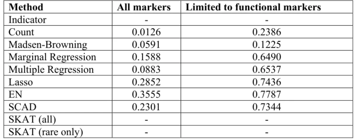
Table 4.1 - Average pearson correlation of true and estimated weights ... 53

Table 4.2 - Permuted p-values on positive control gene in real data set ... 56

Table 5.1 - Type I error rates of separate SKAT tests for all methods ... 64

ix

LIST OF FIGURES

Figure 3.1 - Comparison of Power by r ... 32

Figure 3.2 - Comparison of Power by PAR and d ... 33

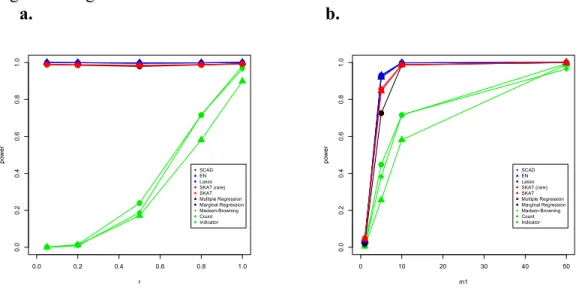
Figure 4.1 - Power Comparison in the Absence of a Bioinformatics Tool ... 49

Figure 4.2 - Power Comparison in the Presence of the Good Bioinformatics Tool ... 50

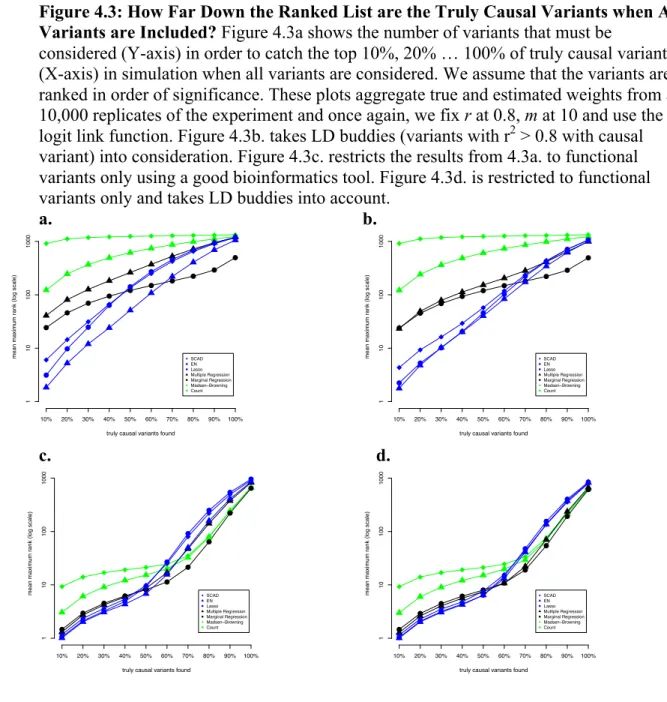
Figure 4.3 - How Far Down the Ranked List are the Truly Causal Variants when All Variants are Included? ... 52

Figure 4.4 - Power Comparison for simulated GWAS data under imputation ... 54

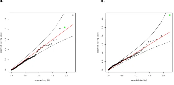
Figure 4.5 - QQ-Plots for p-values in Real Data ... 56

Figure 5.1 - Power for European causal variants ... 66

Figure 5.2 - Power for African causal variants ... 66

Figure A.1 - Complete power results for all link functions and all values m ... 70

Figure A.2 - Complete power results for all linking functions and all values of r ... 71

Figure B.1 - Complete power results for African causal alleles over all values of m ... 72

Figure B.2 - Complete power results for African causal alleles over all values of r ... 73

Figure B.3 - Complete power results for European causal alleles over all values of m ... 74

x

LIST OF ABBREVIATIONS ABCA1 ATP-Binding Cassette Transporter 1

APOA1 High Purity Apolipoprotein A1

APOB High Purity Apolipoprotein B

ATOM Association Test by combining Optimally Weighted Markers

BMI Body Mass Index

CAST Cohort Allelic Sum Test

CEPH Centre de'Etude du Polymorphism Humain

CEU Caucasian European from Utah CNV Copy Number Variant

EN Elastic Net

EREC Estimated Regression Coefficients GRR Genotype Relative Risk

GWAS Genome-wide Association Study

HDL High Density Lipoprotein HG Haplotype Grouping

IFIH1 Interferon Induced with Helicase 1 Kb Kilo-base

LCAT Lecithin—Cholesterol Acyltransferase LD Linkage Disequilibrium

xi MAF Minor Allele Frequency

Mb Mega-base

PAR Population Attributable Risk

RVC Rare Variant Collapsing

SKAT SNP-Set (Sequence) Kernel Association Test SNP Single Nucleotide Polymorphism

T1D Type 1 Diabetes VT Variable Threshold

WDS Weighted Dosage Test

WHG Weighted Haplotype Test for Genotyped SNPs

WHS Weighted Haplotype Test WS Weighted Sum

1

CHAPTER 1: MOTIVATION AND BIOLOGICAL JUSTIFICATION

In this document, we will discuss statistical methods for assessing association between sets of rare genetic sequence variations and complex human traits. This section provides an overview of the biological problems we are interested in and the some of the statistical strategies employed in an attempt to solve them.

To begin, DNA is a double-stranded molecule consistent of four nucleic acid components: Adenine (A), Cytosine (C), Guanine (G) and Thymine (T). DNA is found in the nucleus of the vast majority of plant and animal cells and has been compared to a blueprint for the organism in which it is found. Humans have 22 autosomes, in addition to the sex chromosomes X and Y and mitochondrial DNA, accounting for over 5 billion base pairs in total. We will consider primarily autosomal DNA, for which each individual possesses two copies, one inherited maternally and the other paternally. Over 99% of the DNA sequence is the same across humans (Ohno, 1972), however there are a large number of ways in which human DNA sequence can differ from one another in a single region including microsatellites, copy number variations (CNVs), insertions, deletions, inversions and single nucleotide polymorphisms (SNPs). Any one of these can be called a genetic variant, meaning that it contains a sequence of nucleic acids that is different from the consensus sequence or from what is most common.

2

allele frequency (abbreviated MAF) near 0.5. Because of this, a great deal of genetic variation can be measured by a relatively small subset of these SNPs. In the

1990’smicroarray technologies from companies like Affymetrix and Illumina began to capitalize on these common SNPs in the form of genome-wide SNP platforms. Today these technologies can accurately assess up as many as 1 million pre-selected SNPs [e.g. the Affy Axiom or Illumina 1M], however these technologies are limited in that they cannot discover new variants. Though rare variants outnumber common ones (1000 Genomes Consortium et al., 2010; Mathieson & McVean, 2012), rare variants are seldom included in GWAS panels since they contain little information in relatively small sample sizes. This stands to reason since a marker that is not polymorphic or barely polymorphic in a sample provides little or no statistical power to detect association between the single SNP and the outcome of interest.

3

to elucidate these associations. (Sullivan, 2012) The GWAS study design remains popular, partially due to the emergence of genome imputation for variants not typed. Though rare variants are not typed by the GWAS chips themselves, imputation methods use information from an outside panel such as HapMap or 1000 Genomes to predict the genotypes of markers not in the GWAS panel, including some rare variants, via Markov Chain Monte Carlo (Y. Li, Willer, Ding, Scheet, & Abecasis, 2010; Y. Li, Willer, Sanna, & Abecasis, 2009; Marchini & Howie, 2010).

From 2009 to the present, “next generation” sequencing technologies have brought the cost of whole exome and whole genome sequencing down to hundreds of dollars per sample. These rapid advances in technology allowed investigators to collect larger samples (hundreds or thousands of individuals) that evaluate every base of the genome (or exome), which was previously unimaginable due to cost. Investigators can now evaluate thousands of known rare variants and discover previously unknown variants with these technologies. However, for rare variants, evaluating each variant independently as in GWAS analysis requires a sample size far greater than even these studies can provide. Further if, a variant is unique to one individual, or “private,” no study design will discover this causal relationship if each variant is evaluated one at a time. Because of this, the idea of combining information from multiple variants across a genomic region, gene or pathway became increasingly popular.

4

data from a single ancestral population, this does not change the conclusions greatly; however, when two or more populations are present in the study sample these differences can quickly lead to incorrect results. In particular, populations in which more than one ancestral population’s genetic contribution is present in most or all of the individuals, e.g. African American or Hispanic populations, can be especially complicated. Such

populations are known as admixed populations and many methods have emerged to adjust for the complexity they bring to genetic studies.

This compilation of projects attempts to survey and compare the methodology of several existing methods for the aggregation of rare variants across a genomic region (e.g. gene, exon, pathway). We also aim to improve upon some of these methods and adapt them for use in admixed populations. The next section deals with the history rare-variant collapsing methods and their evolution from simple counting methods, to more complex systems of weighting that utilize phenotype information, and finally, to similarity-based methods which use more complex statistical techniques to assess genomic similarity between individuals and their trait of interest.

The third chapter proposes two methods, a weighted haplotype-based approach and an imputation-based approach, to test for the effect of rare variants with GWAS data. Both methods can incorporate external sequencing data when available. We evaluated our methods and compared them with methods proposed in the sequencing setting through extensive simulations. Our methods clearly show enhanced statistical power over existing methods for a wide range of population-attributable risk, percentage of

5

collected by the Wellcome Trust Case-Control Consortium. Our methods yield p-values on the order of 10-3, whereas the most significant p-value from the existing methods is greater than 0.17. Therefore, we demonstrate that the evaluation of rare variants with GWAS data is possible, particularly when public sequencing data are incorporated. This work was published in the American Journal of Human Genetics in 2010 (Y. Li, Byrnes, & Li, 2010).

The forth chapter presents a systematic evaluation of multiple weighting schemes through a series of simulations intended to mimic large sequencing studies of a

quantitative trait. We evaluate existing phenotype- independent and phenotype-dependent methods, as well as weights estimated by penalized regression approaches including Lasso (Tibshirani, 1996), Elastic Net (Zou & Hastie, 2005), and SCAD(Xie & Huang, 2009). We find that the difference in power between phenotype-dependent schemes is negligible when high-quality functional annotations are available. When functional annotations are unavailable or incomplete, all methods suffer from power loss; however, the variable selection methods outperform the others at the cost of increased

computational time. Therefore, in the absence of good annotation, we recommend variable selection methods (which can be viewed as “statistical annotation”) on top of regions implicated by a phenotype-independent weighting scheme. Further, once a region is implicated, variable selection can help to identify potential causal single nucleotide polymorphisms for biological validation. These findings are supported by an analysis of a high coverage targeted sequencing study of 1,898 individuals.

6

7

CHAPTER 2: LITERATURE REVIEW

This section presents a partial review of many of the papers previously published on the topic of collapsing information across rare variants. It is by no means complete since the number of these papers is quite large; however, it is an attempt to show the development of several methods used to attack this problem. Mathematical notation between the works discussed here is also quite diverse, so n the description of many of these works, some of the mathematical notations (variable names, etc.) has been altered slightly to keep the notation as consistent as possible throughout this document.

2.1 Early Methods

Before the advent of high-throughput genomic sequencing, it had been

hypothesized that collections or combinations of rare variants could be responsible for some of the heritability in human complex traits. When GWAS and other studies turned up promising candidate genes, many researchers invested in re-sequencing and other molecular experiments in order to learn more about these candidates. The first methods for association of rare genomic variants arose from the need to analyze these data.

Well before the rise of “next generation” genome sequencing technologies,

8

common in the low HDL group as compared to the high HDL group, most notably in

ABCA1, (p<0.0001). The investigators reported that one in six individuals with low HDL

had a rare mutation in ABCA1 or APOA1 and went on to replicate these findings in a Canadian sample, thus making a strong case for the involvement of rare sequence variants in complex disease. These investigators did not develop a novel statistical method for assessing the combined effects of rare variants on the genome-wide scale, but they did demonstrate the potential impact of considering associations with combinations of rare variants. Note also that the rare variants were found primarily in the low HDL group, suggesting that these variants exhibit a protective effect. It had been previously suggested that genetic variants can, in most cases, be assumed to have null or deleterious effect. Variants of protective effect were (and are still) considered the exception, rather than the rule. However, the results of this study show the importance of detecting association between genetic variants and human phenotypes in either direction.

As the interest in rare variation grew, so too did the interest in capturing their associations statistically. An approach similar to that described above was formalized by (Morgenthaler & Thilly, 2007). In their manuscript, the authors emphasized the

9

test (CAST). Note that this test only compares counts of rare alleles, and so information must be pooled across individuals and across markers.

In 2008, Li and Leal proposed the Combined Multivariate and Collapsing (CMC) method to collapse across variants across genomic regions, functional groups, MAF categories or other groupings (B. Li & Leal, 2008). These authors advocated first splitting the M markers into k groups (for example, by MAF bin) and then using a collapsing method in which, for each individual i, in the set of variants under study, Li and Leal suggested computing Xi as follows,

Xi =

1, 0,

rare variants present rare variants absent ⎧

⎨ ⎪ ⎩⎪

so that any individual with rare variants present was given weight 1 and all others have weight 0. This reduced the dimension of the multivariate test from M to k, making a multivariate test feasible where it may not otherwise be. Unlike the approach of

(Morgenthaler & Thilly, 2007), Li and Leal collapsed information across markers, within individual, for each group k. The authors reported good results for situations in which one or more rare variants in the same group were truly deleterious.

10

locus, which was assumed to be un-typed. It did so by capitalizing on the correlation or linkage disequilibrium (LD) structure of the region. Suppose that the external data set has

Me markers and Me > M. For each pairwise combination of variants in the original data set, j∈{1, 2,...,M}, and each marker in the external data set l∈{1, 2,...,M_e}, the weight

wl_{j is computed,}

wj

l ₌ Δj l

q_j(1−q_j),

where qj is the minor allele frequency at variant j from the reference data and Δj l _{is the}

linkage disequilibrium (LD) coefficient for markers l and j. Then, for each of the markers in the external data set, l∈{1, 2,...,Me} the authors computed the score,

S_il = 1

m wj

l x_ij j=1 M

∑

so each individual had Me scores. Then the authors performed principal component analysis (PCA) on these scores, thus reducing the dimension of the problem significantly. The principal components were then tested for association with the trait by conventional regression methods without permutation. ATOM performed well compared to other previous methods in terms of power and also performed well when compared to simple haplotype approaches not discussed here.

11

estimated minor allele frequency (MAF) of marker j among controls, denoted qj, where,

qj=

xij

i=1 Ncontrol

∑

Ncontrol+2

to construct weights, wˆj= Ntotalqj(1−qj) so that, the rarer the allele, the

smaller the quantity wˆ_j. Madsen and Browning then computed the genetic scores for

each individual, denotedSi= xij

ˆ

wj j=1

M

∑

came from the variants rarest among controls. This stands to reason since deleterious alleles may confer a selective disadvantage and therefore be less common in the

population than neutral or beneficial ones. Madsen and Browning performed a Wilcoxon Rank Sum test on the collection of Si’s to assess significance. The many simulations presented in the Madsen and Browning manuscript show the Weighted Sum (WS)

method distantly outperforming CAST, CMC and single variant tests in terms of power to detect rare variant association in a number of situations. They also demonstrated their methods’ improved power by applying it to the ENCODE data.

In the following year, Price et. al. proposed a similar method to allow for an unknown threshold on MAF, denoted T, below which variants may be substantially more indicative of a functional variant (Price et al., 2010). As motivation for the idea, Price, et. al. first constructed a weighted sum with a fixed threshold, T, and constructed genetic

scores, Si = ξj(2−xij)yi j=1

M

∑

12 values. The Z-score Z(t) is constructed,Z(t)= ξj

T

(2−xij)(yi−y)

i=1

N

∑

M

∑

N _i=1yi

N

∑

is the mean of the outcomes yi. The value of T that maximizes Z(t) in each case was then chosen as the threshold. Because of this step, the Wilcoxon Rank Sum test was no longer valid and statistical significance needed to be assessed by permutation. The authors found their VT approach had greater power than WS and fixed-threshold methods in

simulations for both dichotomous and continuous outcomes. (Price et al., 2010) also applied their VT method to Polyphen-filtered data (Ramensky, Bork, & Sunyaev, 2002) and found a greater improvement in power with the addition of good bioinformatics data.

Also in 2010, a manuscript in Genetic Epidemiology (Morris & Zeggini, 2010) presented a simple experiment demonstrating the importance of the choice of weighting scheme for these types of approaches and the potential for falsely significant results due to non-causal rare variants. The authors tested two scoring methods, which they call RVT1 and RVT2. RVT1 constructed weights for predefined genomic regions according to the proportion of rare variant sites at which an individual i had 1 or 2 copies of the minor allele, thus fitting the following model.

yi=α+λ

I(xij>0)I(qj<T) j=1

M

∑

I(0<qj<T) j=1

M

∑

+γZi+εi, where

εi

~

N

(0,

σ

2

)

13

yi=α+λI I(qj<T)xij

j=1

M

∑

"

#

$$ %

&

''+γZi+εi, where

ε

~

N

(0,

σ

2

₎

The authors found that the weighting scheme based on the proportion of rare variant sites (RVT1) with one or more minor alleles had equal or greater power to the method that only considers whether rare variants are present or not. Morris and Zeggini demonstrated that this power difference was most pronounced when the number of non-causal rare mutations increases. Since RVT1 gave larger weight to individuals with a larger burden of rare variants, these same individuals were more likely to carry one or more rare deleterious variants.

2.2 Using the outcome to inform choice of weights

Though diverse, the early methods for rare variant association demonstrated the importance of combining the data in an intelligent way, rather than simply searching for the presence or count of rare variants. Many of these methods were devised for

application to GWAS data and GWAS data after imputation using an outside reference panel, as described in the previous section. The advent and refinement of “Next

Generation” sequencing technology only made such methods more appealing and, in a relatively short period of time, a plethora of new methods arose, many of them attempted to directly estimate a weight for each marker by explicitly using the outcome

measurements. In this section, we will outline several such previously proposed methods for binary and continuous outcomes.

14

data. Han and Pan suggested first fitting a series of univariate regression models of the form,

logit Pr(Yi =1)=β0+xijβj

where Yi is the case or control status of individual i, and xij is the genotype for individual i

at locus j as before. From each such model, the estimated coefficient, β_j, and a p-value,

pj, were used to estimate the weight for each marker. First, the genotype data was recoded such that,

xij

* = xij,

2−xij,

if βj ≥0 and pj<α0

if βj <0 and pj<α0

⎧ ⎨ ⎪

⎩⎪

,

where α₀ is a predetermined p-value threshold, so that the coefficient,

ˆ

βc=

x_ij*2β

j j=1

M

∑

i=1

N

∑

xij

*

j=1

k

∑

⎞ ⎠⎟ 2

i=1

N

∑

from the model, logit Pr(Y_i =1)=β₀+ x_ijβ_c

j=1 M

∑

all variants with causal effect had the same odds ratio. The authors tested the hypothesis

H0:βc =0 with the usual score test. Despite the questionable assumption of a constant

15

In 2011, Zhang et. al proposed a similar method that also used the results of single marker tests in to inform the choice of weights for each marker (Zhang, Irvin, Arnett, Province, & Borecki, 2011). Assume single marker tests via linear (for continuous outcomes) or logistic (for binary outcomes) have already been conducted and for each marker, we have an estimate of the coefficient for marker j, bj and the standard error of that estimate, sbj. The investigators proposed fitting the model,

Y_i =α+β w_jx_ij

j=1

M

∑

where xij in the number of minor alleles at locus j for individual i and wj is the weight assigned to marker j determined by,

wj =2{p(t≤tj)−0.5}, with tj =

bj

sbj .

where the distribution of t is determined empirically from all of the single marker tests conducted. The probability p(t≤tj) is a left tail value, and so the test was named the

p-value weighted sum test (PWST). In order to assess significance, the authors simply tested the hypothesis, H0:β =0. PWST was also shown to perform well compared to

phenotype-independent approaches.

In 2011, Lin and Tang rigorously showed that the optimal unbiased weight for

each variant was proportional to the true coefficient βj in the limit. (Lin & Tang, 2011)

Since the coefficient could be estimated from the data, it seemed sensible to set ,

where βˆj is the appropriate estimate of the coefficient βj. However, the authors pointed

out two problems with this approach. First, using these weights, their test statistic T

would not be asymptotically normal and, second, the values of βjˆ were relatively

16

unstable considering that the variants in question are rare and the sample size was finite. The authors instead proposed a compromise in which they fit the model,

Yi=αi0+αi+ βjxij+εi j=1

M

∑

) is assumed and construct weights

, where delta is a known constant. Then the genetic score was constructed, as

in previous methods, S_i = ξ_jx_ij j=1 M

∑

named this method EREC (Estimated Regression Coefficients) and found it performed well is simulations and on real data, though some of the similarity approaches (discussed in the next sub-section) produced smaller p-values when applied to real data. The EREC method cannot be applied in cases where M>N and is not intended to account for variant effects in different directions.

In the same year, a Bayesian method that used the data to directly estimate the weights of the individual markers, in addition to assessing to significance of the association between genotypes and trait (as in EREC), was proposed by (Yi & Zhi, 2011). Since this method was intended for use on case-control data, the investigators

ultimately aim to fit the logistic model, logit Pr(Y_i =1)=β₀+ x_ijβ_j

j=1

M

∑

rewrote as logit Pr(Y_i =1)=β0+β xijα_j j=1 M

∑

estimating the α_j,j∈{1, 2,...,M}, and then testing, H₀:β=0. Yi and Zhi offer a

different solution to the problem of instability for the estimates of the individual weights

17

from (Lin & Tang, 2011) by putting priors on the parameters αj and β. The authors

proposed an informative prior on the αj,

αj ~N(µj,τj 2

), τj 2

~Inv−χ2

(1,s_α2 )

where s_α2 was chosen to be a small value such as 0.5. Yi and Zhi point outed that the

choice of the Student-t priors on αj are designed to better deal with disparate effects.

The prior parameter µj could be manipulated according to the prior knowledge about the

variant j, and though the authors did not do this, they suggested using frequency

distribution or functional credibility to determine the value of µ_j. Because of the rarity

of the alleles in question, the variance of xijα_j

j=1

M

∑

of β could also become unstable, the authors suggested a weakly informative prior on β

β~N(0,τ_β2

), τ_β2

~Inv−χ2

(1, 2.52

)

which was meant to keep the β parameter in a reasonable range. This Bayesian linear

model was fitted using Markov Chain Monte Carlo and showed good results for type I error and power far surpassing any of the phenotype-independent methods discussed in the previous sub-section. This gain in power was particularly noticeable when the effects of the causal variants acted in opposite directions. This method was not, however,

compared to any other phenotype-dependent methods previously discussed. 2.3 Similarity-based approaches: why weight?

18

determining the disease etiology in some cases, simply implicating a gene or molecular target can also be helpful to biological and pharmaceutical researchers. The above

methods directly estimate a weight for each marker, but the following methods are aimed at implicating a genomic region by collapsing sets of markers that tend to be shared across two individuals when the outcomes are also similar.

One of the first of such methods was proposed well before the popularization of “next generation” sequencing techniques by (Schaid, McDonnell, Hebbring,

Cunningham, & Thibodeau, 2005). Schaid and colleagues suggested using a U-statistic of the form,

U_global =

K(x_i,x_i')

i<i'

∑

N

2

⎛ ⎝⎜

⎞ ⎠⎟

= w_j

K(x_ij,x_i'j)

i<i'

∑

N

2

⎛ ⎝⎜

⎞ ⎠⎟

j=1 M

∑

j=1 M

∑

where K(x_i,x_i') is a symmetric kernel function that compares the genotype of individual i

to that of individual i’. Specifically, it is the weighted sum of the variant- specific kernels,

U_j =

K(x_ij,x_i'j)

i<i'

∑

N

2 ⎛ ⎝⎜

⎞ ⎠⎟

.

The authors suggested two kernels with which to quantify the similarity of individual i

19

T-test with good results for power and type I error under most conditions, particularly when the number of risk loci rose above 5.

(Neale et al., 2011) also suggest a method to test for any association between a set of genotypes and phenotype rather than individually estimating weights for each marker. For motivation, the authors used the example of set of M coins that could be either fair or biased. Each coin could land as either a case or a control and, if the coin was fair, it would land case and control with equal probability. If the coin was biased (i.e. if the marker is associated with the trait in either direction), they expected the coin to land preferentially as a case or as a control. Thus, the C_αtests for the presence of biased coins

over the M markers, rather than a test for single biased coin. The C_α test statistic

compares the variance of each observed count with the expected variance and then sums over all variants.

T = [(x_case,j−x_total,jp₀)2−x_total,jp₀(1−p₀)] j=1

M

∑

where p0 is the expected number of times the minor allele is expected to turn up in the cases, given the number of total copies of the minor allele in the sample and assuming

that the jth marker is like a fair coin, that is p0 =

xtotal,j

2 for xtotal,j ≥2. The obvious

problem with this setup was singleton counts, since they contain no variance information. The authors suggested binning all of the singleton counts into one category and

proceeding as if they were all from one marker. The quantity T was then normalized and compared to a one-tailed normal distribution. The C_α test performed well in terms of

20

tails that expected, particularly when the sample size is small. Further, this test assumed independence between all variants and for all these reasons, the authors suggested using permutations to assess significance particularly in the presence of LD or when sample size is small.

Later in 2011, Wu and Lee et. al. suggested a more general test with an arbitrary weight matrix also using kernel methodology to compare the genomes of all N samples called SKAT (Wu et al., 2011). As with many of the methods considered above, SKAT aimed to fit a model of the form, Yi =µ+βX that may or may not also have covariates

included in the µ component. They proposed a statistic Q of the form,

Q=(Y −µˆ)'K(Y−µˆ), where K=XWX'

in which X is the N×M matrix of minor allele counts, as before and W is a matrix of weights that can be specified by the users. Wu, Lee and colleagues explored several kernels to incorporate information from various data types to provide a more powerful test. The matrix K was constructed to measure the pairwise genotypic similarity between every two individuals in the sample. The matrix W quantifies the degree of importance each variant. In the absence of a user derived weight matrix, the SKAT authors

recommend using a matrix K such that K(x_i,x_i')= w_jx_ijx_i'j j=1

M

∑

between variants are present (linear kernel) and K(xi,xi')= 1+ wjxijxi'j j=1

M

∑

⎛ ⎝⎜

⎞ ⎠⎟ 2

for when

there are interactions between variants (quadratic kernel). They suggested choosing the weights according to w_j =Beta(q_j,1, 25) where qj is the MAF of variant j, as before. The

21

advocate this method over the C_α test because it can easily account for covariates and

interactions between variants.

Interestingly, the SKAT authors noticed a drop in power when the true situation (unknown in the case of a real study) was similar to that in which the Madsen &

Browning method (Madsen & Browning, 2009) is ideal. That is, situations where the trait was influenced, not by a particular subset of rare genetic variants, but by the number of deleterious, rare “hits” observed in the region. In 2011, Lee and colleagues proposed SKAT-O to optimize the test, even if this was the case (Lee et al., 2012). SKAT-O performed both the SKAT test and the burden test and produces a weighted sum of the two. In situations where the SKAT statistic would be most powerful, SKAT-O lost very little power in comparison to SKAT; however, SKAT-O demonstrated a marked

22 CHAPTER 3: WHAIT

3.1 Introduction

In this chapter, we propose two methods to search for the aggregated effect of rare variants with GWAS data. Our approaches do not rely on the availability of external sequencing data, but they can incorporate such information when available. Moreover, our methods make no assumption on the direction of association of rare alleles with disease risk. We applied our methods, along with existing methods proposed in the sequencing context, to simulated data sets. Our methods demonstrated better performance across a wide range of scenarios with an average power improvement of 8.6% (31.6%) in the absence (presence) of external sequencing data. We also applied our methods to the Wellcome Trust Case-Control Consortium (WTCCC) type 1 diabetes (T1D) GWAS data set in the IFIH1 gene region, where both common and multiple rare variants have been found to influence the risk of T1D (Barrett et al., 2009; Nejentsev, Walker, Riches, Egholm, & Todd, 2009; Smyth et al., 2006).

3.2 Methods

3.2.1 Weighted haplotype score test

Our first test is a weighted haplotype test. Assume a sample of N diploid individuals is collected, among which _Ncs are affected cases and Nct are unaffected

controls. Let m denote the number of genotyped markers in a region of interest. Further

23

Hi = {Hi,1, Hi,2} are the two haplotypes carried by the ith individual, consisting of the m

markers in the region. For each individual i, we define a weighted haplotype score as follows:

WHS_i= W_H

ij j=1

2

∑

in which the sum is taken over the two haplotypes of individual i. Wh stands for the weight of haplotype h and is defined as

Wh =I(h∈C)⋅(−1)

I(h∈P)⋅

Sh,

in which C is the set of disease-contributing haplotypes including both risk and protective haplotypes, P is the set of disease-protective haplotypes (note that P is a subset of C), and

Sh is a score assigned to haplotype h. Following the weighting scheme proposed by Madsen and Browning (Madsen & Browning, 2009) for SNPs, we define Sh as

Sh = Nct⋅fct,h⋅(1− fct,h),

in which fct,h denotes the adjusted frequency of haplotype h among controls and is defined as

fct,h =

Cct,h+1

2(Nct+1)

,

24 according to the formula below:

h∈C

h∈P

if if

fcs,h

tr −

fct,h

tr >µ fct,h

tr

(1− f_ct,htr

)

2Nct

tr ,

fcs,h

tr ₋

fct,h

tr _<−µ fct

tr₍₁₋

fct

tr )

2N_cttr ,

⎧

⎨ ⎪ ⎪⎪

⎩ ⎪ ⎪ ⎪

(Equation 1)

with tr standing for “training set.” Here, µ is a constant that is determined by a

pre-specified type I error rate. For example, µ= 1.28 (1.64) corresponds to a type I error of

0.2 (0.1). Following (Zhu, Feng, Li, Lu, & Elston, 2010) we set µ= 1.28 and randomly

selected 30% of the samples for training in the analysis.

25

alone or to haplotypes including additional markers via incorporation of external reference data.

3.2.2 Weighted dosage score test

Our second test is a weighted imputation dosage test. Following the notations defined above, we assume that there are a total of M markers genotyped or sequenced after the incorporation of one or more external data sets, e.g. the International HapMap Project (Frazer et al., 2007; International Hapmap Consortium, 2005) or the 1000

Genomes Project (Kaiser, 2008). We have previously described a hidden Markov model-based method that imputes untyped markers in study samples by exploiting external data as reference, which was implemented in software MaCH and has become standard in GWAS analysis (de Bakker et al., 2008). Let D = (D1, D2, ..., Di, ..., DN)t _{denote the}

dosage matrices across M markers for the N study subjects, in which Di = (Di,1, Di,2, ...,

Di,j, ..., Di,M) denotes the dosages of the ith individual. Here Dij is the dosage for the ith

individual at marker j, which is defined as the expected number of the rare allele at marker j. Now we define the weighted dosage score for each individual i as

WDS_i= I(j∈M_C)⋅(−1)I(j∈MP)⋅_D

i,j

j=1 M

∑

in which the summation is taken over all M markers with genotype dosage scores. Here MC is the set of markers with the rare allele that contributes to disease risk, and MP is the

26

sequencing context. (1) Weighted SNP Test (denoted by WS) (Madsen & Browning, 2009) is a weighted- sum method in which rare alleles are aggregated and weighted according to a function of minor allele frequency among controls. Despite the fact that the method was proposed as a test for ‘‘rare mutations,’’ it indeed sums over all markers by giving smaller weight to alleles with higher frequency. Although an omnibus regional-based test that evaluates both common and rare variants is some- times desired, here we are interested in a regional-based test for rare variants only, assuming that common variants have been thoroughly evaluated by large-scale GWAS. Because of this, we compared our methods with both the originally proposed test (denoted by WSall) and a

modified version of it (denoted by WSrare), in which only markers with minor allele

27

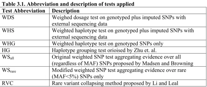
Table 3.1. Abbreviation and description of tests applied Test Abbreviation Description

WDS Weighed dosage test on genotyped plus imputed SNPs with external sequencing data

WHS Weighted haplotype test on genotyped plus imputed SNPs with external sequencing data

WHG Weighted haplotype test on genotyped SNPs only HG Haplotype grouping test orioised by Zhu et. al.

WSall Original weighted SNP test aggregating evidence over all

(regardless of MAF) SNPs proposed by Madsen and Browning WSrare Modified weighted SNP test aggregating evidence over rare

(MAF<5%) SNPs only

RVC Rare variant collapsing method proposed by Li and Leal

3.2.3 Simulation Setup

28 platform.

Within each simulated 1Mbregion, we picked an ~50 kb region as the causal region in which we assume only rare variants (variants with population MAF between 0.1% and 5%) contribute to the disease risk. We randomly selected d% of the rare

variants in the causal region to be causal, i.e., to influence disease risk. Among these rare variants, we further assume that r% of them increase disease risk, whereas the remaining (100 – r)% decrease disease risk. To ensure that each variant only has a small

contribution to the overall disease risk, we followed a model similar to that proposed by (Madsen & Browning, 2009). Specifically, the contribution of each causal variant j to the overall genotype relative risk (GRR) is defined as:

GRRj =

PAR

(1−PAR)⋅MAF_j +1

⎛ ⎝⎜

⎞ ⎠⎟

(−1)I(ξj=1)

,

in which PAR is the population attributable risk and ξ_j =1 indicates that the rare allele of

marker j decreases disease risk. Following (Madsen & Browning, 2009), we used the same marginal PAR for each causal variant, which intrinsically assumes that alleles with lower frequency have higher GRR than alleles with higher frequency. In our 50 kb core region, there are ~500 SNPs with MAF < 5%. To generate the chromosomes for an individual, we randomly selected two chromosomes {H1, H2} from the remaining 9000 chromosomes that were not selected as external reference. The disease status of the individual was assigned according to

P(affected| {H₁,H₂})= f₀× GRR_jI(Hk,j=aj)

j=l mc

∏

2

∏

29

5% were also evaluated and resulted in similar patterns but with slight power loss), mc is

the number of causal SNPs, and aj is the rare allele of SNP j. Sampling was repeated until

the desired number of cases and controls was reached. In our simulations, d took values from 10% to 50% by an increment of 10%. Among the disease risk influencing loci, we set the value of r, the percentage of rare alleles increasing disease risk, at 5%, 20%, 50%, 80%, and 100%, respectively.

For each of the 100 regions, two independent data sets with 1000 cases and 1000 controls were simulated with the model described above. In addition, five independent null data sets of the same sample size were simulated, assuming no genetic effect by randomly sampling 4000 chromosomes (i.e., 2000 individuals) from the pool of 9000 chromosomes. Average power was estimated based on the 100 regions, which represent a wide range of LD patterns. To account for local LD differences, we permuted each of the null sets 200 times to obtain region-specific empirical significant threshold. For the weighted haplotype analysis, we considered two versions: WHG, which uses haplotypes consisting of GWAS SNPs only, and WHS, which uses haplotypes encompassing both genotyped and imputed SNPs. For both the weighted haplotype tests and the weighted dosage test, untyped SNPs with Rsq (estimated imputation quality) < 0.3 were discarded from subsequent analysis (Y. Li et al., 2009).In all analyses, we used haplotypes

reconstructed from the unphased genotypes and imputed genotypes for markers that are not included on the GWAS chip. Our methods (WHG, WHS, and WDS), together with WS_all, WS_rare, HG, and RVC, were applied to the 1000 null data sets within each region to

30 3.3 Results

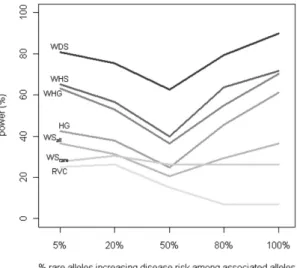
Figure 3.1 shows the empirical power of our methods relative to the other four

methods proposed in the sequencing context as a function of r, the proportion of rare alleles increasing disease risk, which ranges from 5% to 100%. We fixed PAR at 0.5% and d (percent of disease-influencing rare variants) at 50%. Although the synergy assumption is more reasonable for rarer alleles than for common alleles because rarer alleles tend to disrupt gene function, our knowledge regarding the direction of rarer alleles is still limited. Therefore, methods robust to such an assumption are desirable. Although all methods have decreased power when rare alleles work in different directions, our methods performed better by explicitly modeling the direction of association. For example, compared with the haplotype grouping (HG) method, the advantage of our weighted haplotype method (WHG, on GWAS SNPs only without the aid of external sequencing data) manifests more when a larger proportion of the rare alleles is protective: power gain is 9.1% when all of the rare alleles at disease-

contributing loci increase disease risk, and the power gain increases to 20.7% when only 5% of the rare alleles increase disease risk.

Our proposed tests increase power through two different mechanisms: by using haplotypes to better capture information for rare variants (mostly untyped in GWAS) and by using external sequencing data to impute rare variants. Let us consider the first

mechanism by examining tests on GWAS data alone, namely WHG, HG, WSall, WSrare,

31

viewed as special cases of WDS, where the dosages only take values 0, 1, or 2 at directly genotyped markers. Therefore, at the GWAS level, haplotype-based methods are

preferred over single-marker dosage-based tests. This is because causal rare variants are better captured by haplotypes constructed from GWAS SNPs than by those SNPs themselves. Between the two haplotype-based methods, our weighted haplotype method (WHG) increases power by an average of 13.2% over HG by weighting individual haplotypes (instead of lumping them together into groups) and by explicitly modeling the direction of association.

32

Figure 3.1. Comparison of Power by r: Percent of Rare Alleles in the Causal Region that Increase Disease Risk Power of all tests was assessed at the 5% level by using empirical significance threshold determined by 1000 null data sets per region. 50% of the rare alleles in the causal region were assumed to contribute to disease risk (i.e., d fixed at 50%), and the PAR of each contributing SNP was fixed at 0.5%.

Figure 3.2 shows the power of different tests under situations with varying PAR

and varying percentage of disease-contributing rare variants. We fixed the value of d

(percentage of rare alleles influencing disease risk) at 100%. The value of r (percent of causal alleles increasing disease risk) was fixed at 50% for Figure 3.2a, and the per SNP PAR was fixed at 0.5% for Figure 3.2b. Although the power decreases with decreasing PAR or decreasing percentage of disease-contributing variants for all methods, our WHG and WHS are comparable, if not slightly better, than other alternatives, and our WDS is more powerful than the other methods by utilizing sequencing information from external data and explicitly modeling the SNP-level dosages.

We note that tests on rare GWAS SNPs only (WSrare and RVC) are less powerful

33

sequencing context, are thus not suitable for analyzing GWAS data.

Figure 3.2. Comparison of Power by PAR and d: In figure 3.2a, power of all tests was assessed at the 5% level by using empirical significance threshold determined by 1000 null data sets per region. 50% of the rare alleles in the causal region were assumed to contribute to disease risk (i.e., d fixed at 50%), and all contributing rare alleles were assumed to increase disease risk (i.e., r fixed at 100%). In figure 3.2b, power of all tests was assessed at the 5% level by using empirical significance threshold determined by 1000 null data sets per region. All rare alleles in the causal region were assumed to increase disease risk, and the PAR of each contributing SNP was fixed at 0.5%.

a. b.

34

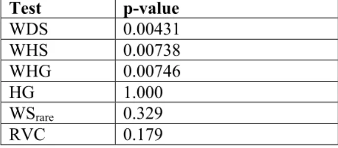
2009; Smyth et al., 2006),we restricted our analysis to SNPs or haplotypes with frequency < 5% to rule out signals due to LD with rs1990760. Our goal is to assess whether there is any residual association with T1D because of rare variants, which have been ignored in the previous GWAS analysis. We used the March 2010 release of 60 CEU individuals from the 1000 Genomes Project as reference for imputation. We used SNPs in the ~50 kb IFIH1 gene region plus 2 Mb flanking on each side for phasing and imputation. Again, we discarded imputed SNPs with Rsq < 0.3. For the haplotype grouping method, the original test failed in this data set because rare alleles in IFIH1 are associated with decreased risk of T1D. P-values based on 100,000 permutations are shown in Table 3.3. The p values from our methods are in the order of 10-3, whereas the most significant p value from existing methods is >0.17. This example clearly

demonstrates the importance of using appropriate methods when searching for the effect of rare variants with GWAS data.

Table 3.2. Allele frequencies of six polymorphic SNPs in IFIH1

SNP 58C NBS T1D

rs3747517 27.66% 26.31% 24.16%

rs41463049 1.12% 1.06% 1.02%

rs6432714 1.18% 1.06% 1.02%

rs13023380 48.88% 47.46% 45.24%

rs7559193 0.17% 0.10% 0.00%

rs12479125 1.18% 1.06% 1.02%

Table 3.3. Permutation p-values based on 10,000 permutations, for the association of rare variants in IFIH1 with T1D risk in WTCCC data set

Test p-value

WDS 0.00431

WHS 0.00738

WHG 0.00746

HG 1.000

WSrare 0.329

35 3.4 Discussion

In summary, we have proposed two tests to assess the impact of multiple rare variants on disease risk. We show through simulations and a real-data example that by maximally extracting information from GWAS data, as well as the incorporation of publicly available sequencing data, our methods provide an intermediate solution for the analysis of rare variants before study-specific sequencing data become available. Our results suggest that at the GWAS level, haplotype-based methods are more powerful, but at the pseudo-sequencing level (i.e., GWAS data imputed with publicly available

sequencing data), a test based on weighted sum of single-marker dosages is more powerful.

36

genome, and our knowledge regarding their impact on phenotypic variations is still limited. Third, traditional association tests are suitable for the analysis of common variants but are generally underpowered for the analysis of rare variants. By utilizing LD information and incorporating publicly available sequencing data, we show that hunting for rare variants with GWAS data is possible.

Our methods are proposed for GWAS data, which are still the most commonly available type of data for gene mapping studies. In both our simulations and the real data analysis of T1D with gene IFIH1, we only have GWAS data on the study subjects. We compared our methods with alternatives proposed for sequencing data and demonstrated that methods that are specifically targeted for the analysis of rare variants in GWAS settings such as ours perform much better than methods that are developed for

37

individuals with constructed haplotypes encompassing both common and rare variants from an independent set of FUSION individuals (of varying sizes) as reference. We found that imputation quality for rare variants improves when the sample size in the

reference panel increases. For example, the accuracy among the heterozygotes (r2) increases from 83.4% (74.3%) to 97.0% (92.9%) when the number of reference haplotypes increases from 60 to 1000.

Our methods and others evaluated in this study were developed for the analysis of rare variants, but we have found that inclusion of common variants can increase the power (data not shown). This is demonstrated by the superior performance of WSall (test

that includes all variants) over WSrare (test that only includes rare variants), even though

only rare variants that contribute to disease risk were included in our simulations. This is not entirely surprising, because common variants or haplotypes can carry some

information of untyped rare variants. One major issue of including common variants in testing is misclassification, that is, inclusion of variants that do not contribute to disease risk. However, by searching for frequency difference in a training set, our methods can alleviate this misclassification issue. In general, we recommend testing common variants first, for instance, via standard single-marker test. If there is no evidence of association with common variants, we then search the entire MAF space for the effect of rare variants. When common variants are found to be associated (such as in the IFIH1

example), we should restrict our attention to rare variants or haplotypes only to alleviate the residual effects of common variants.

38

For real-life GWAS data, we recommend performing the tests for all known genes if no prior knowledge exists or for a list of one or more candidate genes in the presence of such knowledge. We note that the weighted dosage-based test is more flexible than the

haplotype-based test in that it can be used to test for an arbitrary set of SNPs (for example, non-synonymous rare SNPs in a pathway), which may involve SNPs on different chromosomes.

One issue with the haplotype-based test is that the haplotypes are not known but instead are inferred with uncertainty. Fortunately, most phasing methods, including PHASE and MaCH, can estimate the probabilities of possible haplotype configurations for each individual in addition to providing the best-guess haplotypes. With these estimates, we can easily model the phasing uncertainty into our weighted haplotype test by allowing possible haplotype configurations of each individual to contribute to the haplotype frequency estimates, as well as to the weighted haplotype score, according to their estimated probabilities. An alternative approach is to perform multiple imputation on 5–10 imputed data sets (Little & Rubin, 2010).Note that each imputed data set has to be drawn from a different posterior distribution to ensure proper multiple imputation. This can be achieved either by imputing from different reference sets (for example, from bootstrap samples of the HapMap or 1000 Genomes reference set) or by drawing from different iteration in a full Bayesian framework in which the model parameters are also up- dated in each iteration. Neither approach had noticeable impact on the IFIH1 real data set, but further work is warranted.

39

each individual and assess the association between the genetic score and phenotype of interest. The genetic score is a weighted sum of contributing SNP dosages or haplotypes. Although the weights are defined for dichotomous trait in this work, we can easily extend the work to quantitative traits by first estimating the weights, for the very simple

40

CHAPTER 4: FUNCTIONAL AND STATISTICAL ANNOTATION 4.1 Introduction

In this chapter, we present an evaluation of multiple weighting schemes through a series of simulations. We evaluate several existing phenotype-independent (Cohen et al., 2004; Madsen and Browning, 2009; Morgenthaler and Thilly, 2007) and -dependent weighting schemes (Wu et al., 2011; Xu et al., 2012), as well as weighting schemes determined by linear regression, penalized regression and variable selection methods, including Lasso (Tibshirani, 1996), Elastic Net (Zou and Hastie, 2005) and SCAD (Xie and Huang, 2009). We conduct simulations under a variety of scenarios with different numbers of true causal variants, mixtures of direction of effect and availability of functional information, mimicking sequencing studies of a quantitative trait. We then apply each of these methods to a set of high coverage targeted sequencing data (Nelson et al., 2012) of 1898 individuals from the CoLaus population-based cohort (Firmann et al., 2008).

4.2 Methods

4.2.1 Statistical Methods

41

there are N individuals under study, indexed by i, and for each individual we have M

variants in the region or variant set, indexed by j.

First, we examine three approaches that are independent of the observed

phenotype. The first of these is a simple indicator of whether or not rare variants (minor allele frequency, MAF < 0.01) are present in the region (Cohen et al., 2004). That is,

where xij is the number of minor alleles observed for individual i at variant j.

is the estimated MAF of variant j in the data with pseudo counts and Q is

the MAF threshold. In this work, we consider Q=0.05.

Second, we examine a count approach which assigns a higher score to individuals carrying a larger number of rare alleles (Morgenthaler and Thilly, 2007);

Si = I( ˆqj <Q)xij

j=1 M

∑

with xij being the count of rare alleles for individual i at variant j and being the

estimated MAF, as defined above.

We also consider the approach proposed by Madsen and Browning (Madsen and Browning, 2009) where the weight for variant j is a function of the minor allele frequency (MAF):

, where

Si=I I( ˆqi<Q)xij >0

j=1 M

∑

#

$$ %

& ''

ˆ

q_i=

xij+1

i=1 N

∑

2N+2

ˆ

q_j

1 M

i j ij

j

S ξ x

=

=

∑

1

42

with xij and as above. In the original Madsen and Browning framework for

case-control studies, MAFs are estimated using case-controls only. However, in this paper, the outcome of interest is quantitative and we estimate MAF using the entire sample, which makes the method phenotype-independent in this context.

We also consider phenotype-dependent regression-based methods. First, we examine the performance of marginal regression coefficients. That is, we fit the simple linear regression model for each variant j separately and independently and

then take the fitted values to be our weights.

, where , the MLE of for the model above.

Though imperfect, this weighting scheme allows investigators to test for associations with multiple rare variants in cases where N < M and begin to follow up on individual variants that may potentially be of interest.

Second, we consider weights from ordinary multiple regression, modeling all of the M variants simultaneously. That is, we fit the model , where the (i, j)th

element of the matrix , the minor allele count for individual i at variant j. We then

take Si to be as above, with the fitted values from this multiple regression, (Lin

and Tang, 2011; Xu et al., 2012).

We also consider weights from several variable selection methods. Such methods are appealing since we expect the majority of rare variants not to influence the quantitative trait of interest. Use of penalized regression is therefore expected to reduce the number of non-zero weights. Similar strategies were recently proposed in the context of rare variant association testing (Turkmen & Lin 2012; Zhou, 2010). In penalized

ˆ

q_j

Y =x_jβ+ε



β_j

1 M

i j ij

j

S ξ x

=

=

∑

Y = X

β ε

ij

X =x

ˆ

43

regression, we solve for the which best fit the data, subject to some constraint(s) or

penalty. That is, instead of minimizing the sum of squared error, , we aim to minimize the sum of squared errors and an additional penalty term, . In general, the greater the number of parameters included in

the model, the greater the penalty. A number of penalty functions have been proposed and extensively studied in the recent statistical literature (Heckman & Ramsay 2000; Hesterberg et al., 2008; Kyung et al., 2010; Wu & Lange 2008). Of these, we chose three: the Lasso which imposes a linear penalty (Tibshirani 1996), Elastic Net (EN) which imposes a quadratic penalty (Zou and Hastie 2005) and SCAD which is designed to penalize smaller coefficients more heavily than larger coefficients (Xie & Huang 2009).

For Lasso and SCAD, only one tuning parameter, λ, is required. We used the R packages lars (Efron, Hastie, Johnstone, & Tibshirani, 2004) and ncvreg (Breheny Huang 2011) with default parameter values, which is to choose the optimal λ among a grid of 100 possible values equally spaced on the log-scale. For Elastic Net, there are two tuning parameters, one for the linear component and one for the quadratic component. The linear term, λ1, is chosen in the same way as the λ parameter for the Lasso and

SCAD methods, discussed above. The quadratic parameter, λ2, was set to 1 in all

simulations and for the real data. We used the R package elasticnet to fit the EN models (Zou & Hastie, 2005). After model fitting, we then use estimated coefficients from each of these variable selection methods as weights. The number of non-zero coefficients included is upper-bounded by 100 for each of these schemes throughout this work.

ˆ β's

(Y−βX)'(Y−βX)

44

Under each weighting scheme examined, we determine the significance of a

genomic region using a score test of the following form: where

in which N is the number of individuals under study, and Yi is the

quantitative trait value for the ith individual. Si is the genetic score for the ith individual, a weighted sum across multiple variants. Specifically, xij is the number of minor alleles observed for individual i at variant j where xij are not normalized. M is the number of variants in the region under study (discovered through sequencing in our context) and ξj

is the weight of variant j under one of the above weighting schemes. The analytical distribution for this statistic is not generally known in this context, so significance must be assessed empirically by permutation.

Additionally, we apply the similarity-based method SKAT (Wu et al., 2011) to each of our simulated data sets and the real data set for comparison. We use weights based on the default Beta distribution implemented in the SKAT package, version 0.79. We will comment in the Discussion section on the conceptual differences between the weighting schemes we consider in this work and the SKAT methodology.

4.2.2 Simulation Setup

We simulate 45,000 chromosomes for a series of 100 50Kb regions with a coalescent model [Schaffner et al. 2005] that mimics linkage disequilibrium (LD) in real data, accounts for variations in local recombination rates and models population history consistent with the CEU samples. We then randomly select 2,000 simulated

chromosomes (forming 1,000 diploid individuals) to mimic a large sequencing study. For each region, we simulate one single pool of 45,000 chromosomes instead of multiple

1

( )

N

i i

i

U Y Y S

=

=

∑

1 M

i j ij

j

S ξ x

=