2017 International Conference on Computer, Electronics and Communication Engineering (CECE 2017) ISBN: 978-1-60595-476-9
The Automatic Model Selection and Variable Width RBF Neural
Networks for Chaotic Time Series Prediction
Peng ZHOU
*and Qi YANG
State Key Laboratory of Optical Communication Technologies and Networks, Wuhan Research Institute of Posts & Telecommunications, Wuhan, 430074, China
*Corresponding author
Keywords: Radial basis function network, Chaotic time series, variable width.
Abstract. This paper investigates the construction of radial basis function(RBF) neural networks, and a new self-adaptive algorithm is presented to achieve chaotic times series prediction. This method is based on an adaptive Orthogonal Least Squares(OLS) algorithm, that the automatic model method can assign an appropriate number of hidden units for the network, and the variable width model may guarantee a natural overlap between kernel functions. The proposed algorithm may specify appropriate number and widths of kernels simultaneously. The augmented algorithms are employed to some examples such as Mackey-Glass mapping in known and unknown noise chaotic dynamical systems. Experimental results show that the proposed algorithm can produce a better prediction.
Introduction
There are many research results about chaos time series prediction due to their wide applicability in many practical systems such as secure communication, chemical reactions, biological systems and information processing. It can be see from them that the key problem of prediction lies in the formation of prediction models. Some classical models, such as auto regressive moving average (ARMA), recurrent neural networks (RNN), and support vector machine (SVM), have been developed for the prediction. Radial basis function (RBF) neural network have been also employed independently or as an auxiliary tool to predict chaotic time series. E.S. Chng et al. proposed a gradient RBF (GRBF) model for chaotic time series prediction.
An appropriate RBF network structure is a key issue because it governs the prediction effect of chaotic time series. However, some well developed RBF algorithms, such as k-means, RAN, RPCL, GAP and its variants, intensively depend on the distribution of the input-output samples; In practical applications, the most important is robustness. they may break down or have improper number of centers when its corresponding parameters or thresholds cannot be specified correctly. A significant contribution to construct RBF networks is made by Chen et al. [1] and Chng et al. Through development of orthogonal least square (OLS) algorithm and its variants also have been proposed. However, The orthogonal subset method cannot realize an self-adaptive RBF neural network. There are two main reasons considered here. The first one is that it is unable perform model selection automatically because the user is required to specify the tolerance , which is relevant to noises and will be difficult to implement in the real system. Another is that the default uniform distribution doesn't accord with the actual situation of chaotic time series.
The rest of the paper is organized as follow. In Section 2, we consider the problem of chaotic time series prediction using an RBF prediction. Section 3 presents the proposed method which is developed to construct an better RBF predictor. Section 4 describes the Mackey-Glass mapping simulations carried out to evaluate the performance of the proposed algorithm.
An RBF Network for Chaotic Time Series Prediction
Prediction Menthod of Chaotic Time Series
According to the Takens [3] embedding theorem, there exists a diffeomorphism such that
1 1
(xi ,...,xi L) ( ,...,xi xi L ), i L
where {xi} is a chaotic time series generated by a D-dimensional nonlinear system. Let H: L 1 be a projection defined by
1 1
( ,..., )L
H x x x
Letf H, then
1
( ,..., )
i i i L
x f x x
where the domain of definition of f is the same the domain of definition of the diffeomorphism.
{xi} is a measurement sequence of the dynamical system.
Reconstructing a chaotic system from its time series measurements is specified by two ingredients. First, we need to determine a suitable embedding dimension L. Many techniques have been to select a suitable L in the literature and we assume that a suitable L is available in the study. Second, a good representation f makes chaotic time series predicting work well.
RBF for Chaotic Times Series Pecification
The radial basis function network offers a viable alternative to the two-layer neural network which is linear in the parameters by fixing all RBF centers and nonlinearities in the hidden layer. So an RBF neural network has a simple topological structure and university approximation ability and can be used as a predictor to model the unknown mapping f.
An RBF predictor, fK, is a linear combination of K RBFs that is
1 1
1
( ) K ( / )
i K i j i j j
j
x f w
x x c
where (||xi-1-cj||/j) is the RBF with center cj and widthj, ||.|| denotes the Euclidean norm. To make fK close to f, the distance between f and fK is minimized with respect to the parameters of fK, that is, cjs, js and wjs. Here the coefficients
wjs (j=1,2,...,K) are chosen by the linear least squares (LS) or Recursive Least Squares (RLS) method.
The Automatic Model Selection and Sel-adaptive Width Algorithm for Better RBF Prediction
The automatic model selection and variable width learning algorithm is employed to realize a better RBF network, in which cost function and the variable width method is incorporated to detect the number of hidden units under considering the real distribution of chaotic time series fully.
Automatic Model Selseciton
In the past decades, some related works of RBFNN have been done toward determining the correct number of clusters or densities along two major lines. The first one is to develop new advanced algorithms that perform clustering without pre-deciding the exact cluster number. For example, the typical incremental clustering gradually increases the number k of clusters under the control of several threshold values. The other direction is to formulate the cluster number selection as the choice of component number in a finite mixture model. There are some information theoretic criteria proposed for model selection accordingly, such as minimum description length (MDL), Akaike information criterion (AIC), Stein’s unbiased risk estimator (SURE) and Bayesian information criterion (BIC) [4]. They have different advantages and disadvantages. MDL fails to indicate an optimal number of hidden units and produces reasonable estimate except for high signal-to-noise ratio (SNR) data, while the number of hidden units determined by BIC still can be consistent with the number of hidden units that yielded the minim mean square error (MSE) for low SNR data. In contrast, AIC yields greater MSE for almost any kind of SNR data. Hence, BIC may generate an accurate estimate of the number of hidden units for all kinds of SNR signals. SURE method proposed by Ghodsi et al. is similar to BIC. They produce the same result if the factor 2 in SURE is replaced by log N (N is the number of observations or the dimension of a given
observation). It means that when N > e2, BIC penalizes complex models more and gives preference to simpler models than SURE. In short, BIC maybe enables us to construct a better radial basis function network nonlinear regression model than other three methods. By extending Schwarz’s basic, S.Konishi et al have presented various types of BIC which cover the evaluation of models estimated by the method of maximum penalized likelihood. In this paper, we extend BIC and use it as a good cost function of constructing RBF network.
An RBF network with too few basis functions gives poor generalization on new data. On the other hand, an RBF network with too many basis functions also yields poor predictions since it may fit the noises in the training data. An RBF network with small number of basis functions yields a high bias and a low variance, whereas network with large number of basis functions yields a low bias but high variance estimator. The best prediction performance is obtained via a compromise between number of basis functions and variances. As can be seen from the expression of BIC, it is an important mechanism in balancing the two above mentioned. Its generic form is
2 log (log )
BIC likG M
where in the case of linear models lik denotes the likelihood of a model estimated by the maximum
likelihood method, G is the dimensionality of inputs. Under the Gaussian model, Schwarz’s
procedure can be written as
2
( ) log( )k log( )
BIC M M S G M
where Sk denotes the standard deviation of training samples. As the latest selected term is added to
uniform distribution of centroids. Unfortunately most real-life problems including the chaotic time series prediction show non-uniform data distributions. In this subsection we give a variable width method to solve the problem. To calculate the local widths of every hidden unit, a pilot density estimate is first computed as [5]:
0 0
( ) (( ) / ) / d
i i j
j i
p x k x x n
where 0 is a global width and the index d is the dimension of the data space {xi}i=1,...,n. The kernel,
K, is taken to be a Gaussian function centered at zero and integrating to one. Based on Eq. (9) local
widths are calculated as:
0
( )xi [ / ( )]p xi
where p(xi) is the estimated density at point xi, is the sensitivity parameter, a number satisfying 0 1(a suggest value for is 1/2 ), is a proportionality constant, which has an effect on the local width. If p(xi)<, (xi) increases relative to 0 implying more smoothing for the point xi, for data points that verify p(xi)>, the local width becomes narrower. A good choice is take as the geometric mean of {p(xi)}i=1...n . It can be written as
1
log n log( ( ))p xi
A particular choice of (xi) is able to perform much better than fixed-widths methods, as they
offer a greater adaptability to the data.
To address the above mentioned problems of global width, this paper presents a new better scheme such that the global width, which is employed in the selection of the network architecture (numbers and selections of nodes) and the model parameters (centers and widths), can be evolved by the differential evolution (DE) algorithm based on an exhaustive search. Currently, there are several variants of DE. The particular variant(PSO-DE) used throughout this investigation is the DE/rand/1 bin scheme. The iterative minimal value of BIC of each individual is a fitness which is used to measure candidate optimality. When PSO-DE is employed to calculation of the local width, the formulation (10) becomes
0
( )xi / ( )p xi
In this way, the molecular can be seen as one parameter evolved by PSO-DE, the parameter of the denominator has no effect on the relative position distribution of (xi). The real value of (xi) is insensitive to it and fine-tuned by the denominator.
Overview of Algorithm
Figure 1. The schematic of learning hierarchy for RBF predictor.
Computer Simulation
In the following, Mackey-Glass chaotic time series is use to test the above algorithm, which is defined as follows [6]:
10
( ) / ( ) / (1 ( ) ) ( )
dx t dtax t x t bx t
When 17, the equation shows chaotic behavior. Higher values of yield higher dimensional
chaos. To make the comparisons with earlier work fair, we chose the parameters of a=0.2 b=0.1. Two hundred data points were generated with an initial condition x(1)=0.1, t(1)=0 and 17 based on the fourth-order Runge-Kutta method. The first 100 data pairs of the series were used as training data, while the remaining 100 were used to validate the model identified.
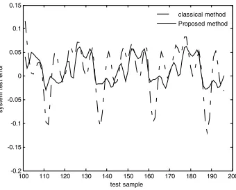
To more clearly test the performance of the new method, we conducted a simple comparative analysis between the proposed method and the orthogonal and uniform width (classical) method. The RBF predictor constructed with the proposed method has 8 centers (the proposed method ( )) while the predictor obtained with the classical method has 20 centers (the classical method (o)) under no noise. The predictor accuracies and error over the validation set was then computed and the results are plotted in Figure 2 and Figure 3, respectively. It can be seen from the two figures that better prediction performance was achieved with the proposed method which achieves a lower approximation error measured by the error calculated over 100 sampled data.
100 110 120 130 140 150 160 170 180 190 200
0.2 0.4 0.6 0.8 1 1.2 1.4 1.6
Input x
O
utp
ut
y
data classical method Proposed method
[image:5.612.225.392.493.628.2]100 110 120 130 140 150 160 170 180 190 200 -0.2 -0.15 -0.1 -0.05 0 0.05 0.1 0.15 test sample sy st em te st e rr or classical method Proposed method
Figure 3. Prediction errors of Mackey-glass mapping under no noise.
The effect of noise on the performance of the new algorithms was analyzed by adding different levels of Gaussian white noise to the training patterns. To do such experiment, the training sets corrupted by the noise standard deviation uniformly chosen in the interval (0.01 0.1) and then both of them were applied to these data samples. The number of hidden units and the network MSE obtained by them are shown in Figure 4 and Figure 5, respectively. It can be seen from the two figures that the proposed algorithm always realized the better prediction with smaller network for different noisy chaotic time series.
0.01 0.02 0.03 0.04 0.05 0.06 0.07 0.08 0.09 0.1
0 1 2 3 4 5 6 7 8 9 10
Noise standard deviation
[image:6.612.223.393.336.470.2]N um ber of hi dden un its classical method Proposed method
Figure 4. Number of hiden units under different noise levels.
0.010 0.02 0.03 0.04 0.05 0.06 0.07 0.08 0.09 0.1
1 2 3 4 5 6x 10
-3
Noise standard deviation
MS
E
[image:6.612.225.392.502.640.2]classical method Proposed method
Figure 5. Comparison of MSE under different noise levels.
Acknowledgment
References
[1] S. Chen, C.F.N. Cowan and P.M. Grant, “Orthogonal least squares learning algorithm for radial basis function networks,” IEEE Trans. Neural Network, vol. 2(2), 1991, pp. 302–309.
[2] Y. Yue, S. Ge, S. Ren and Z. Qian, “Optimal control for wastewater treatment process based on mixed PSO-DE algorithm,” Computer Measurement & Control, vol. 24(2), 2016, pp. 68–70.
[3] F. Takens, “Detecting strange attractors in turbulence,” Lecture Notes in Mathematicks, vol. 898, 1981, pp. 366–381.
[4] S. Konishi, T. Ando, S. Imoto, “Bayesian information criteria and smoothing parameter selection in radial basis function networks,” Biometrika, vol. 91(1), 2004, pp. 27-43.
[5] Z. Yang, Q. Zhao, W. Liu, “Energy based evolving mean shift algorithm for neural spike classification,” 31st Annual International Conference of the IEEE EMBS Minneapolis, vol. 2 (6), 2009, pp. 966-969.