Finite element simulation of machining aisi 1045 steel using uncoated carbide tool

NABILA AFIF BINTI MOHMD ARIFIN

A thesis submitted in partial

fulfillment of the requirement for the award of Master Degree of Mechanical Engineering

Faculty of Mechanical and Manufacturing Engineering Universiti Tun Hussein Onn Malaysia

ABSTRACT

ABSTRAK

CONTENTS

TITLE i

DECLARATION ii

DEDICATION iii

ACKNOWLEDGEMENT iv

ABSTRACT v

ABSTRAK vi

TABLE OF CONTENTS vii

LIST OF TABLES xi

LIST OF FIGURES xii

LIST OF SYMBOLS xiv

CHAPTER 1 INTRODUCTION 1

1.1 Introduction 1

1.2 Problem Statement 3

1.3 Objectives of Study 4

1.4 Scope of Study 4

1.5 Rationale 4

1.6 Overview 5

CHAPTER 2 LITERATURE REVIEW 6

2.1 Introduction 6

2.2 Mechanics of metal cutting 7

2.2.1 Orthogonal cutting 7

2.2.3 Cutting temperature in turning 12 2.3 Minimum quantity lubricant (MQL) 14

2.4 Finite element analysis 16

2.4.1 Finite element formulation 18 2.4.2 Modelling of material properties 20 2.5 Friction model 21 2.5.1 Friction models for machining 22

2.6 Conclusion 24

CHAPTER 3 METHODOLOGY 25

3.1 Introduction 25

3.2 Experimental setup 26

3.2.1 Cutting tool material 26

3.2.2 Workpiece material 27

3.2.3 Machining test and cutting conditions 28 3.2.4 Force measurement 29 3.2.5 Temperature measurement 31 3.2.6 Lubrication technique and cutting fluid

lubricant 34

3.3 FEM simulation of orthogonal cutting 36

3.4 Geometry modeling 36

3.5 Tool-Chip contact and Boundary Conditions 37

3.6 Mesh Generation 39

3.7 Methodology Flowchart 41

CHAPTER 4 RESULT AND DISCUSSION 42

4.1 Introduction 42

4.2 Comparison of FEM results with experimental 43 data

4.2.1 Effect of various friction model 45

4.2.1.2 MQL conditions 49 4.3 Effect of various friction coefficient for MQL 53 4.4 Effect of various heat transfer coefficient for MQL 55

CHAPTER 5 CONCLUSION AND RECOMMENDATION 58

5.1 Conclusion 58

5.2 Recommendation for future works 59

REFERENCES 60

LIST OF TABLES

2.1 Characteristics of synthetic esters and fatty alcohol 15

3.1 Cutting tool geometry 26

3.2 Composition of AISI 1045 27

3.3 Properties of AISI 1045 27

3.4 Summary of cutting conditions 28

3.5 MQL supplying system 34

3.6 Geometry Specification 37

3.7 Friction Models 38

4.1 FEM simulation result for cutting force and temperature compared with experimental data for dry condition 46

4.2 FEM simulation result for cutting force and temperature compared with experimental data for MQL condition 49 4.3 FEM simulation result for cutting force, Fz at different

friction coefficient for MQL condition 53

LIST OF FIGURES

1.1 Turning Process 2

2.1 Orthogonal Cutting Geometry 8

2.2 Oblique Cutting Geometry 8

2.3 Schematic illustration of two-dimensional orthogonal cutting 9

2.4 Thin shear plane model 10

2.5 Thick shear plane model 10

2.6 Cutting (Fc) and thrust (Ft) force components of resultant

tool force (Fr) 11

2.7 Region of heat generation in turning 13

2.8 Lagrangian definition 18

2.9 Eulerian definition 19

2.10 Explanation of contact between two surfaces 21

2.11 Static and kinetic friction 22

2.12 Stresses distribution on rake face 23

3.1 Cutting tool 26

3.2 Workpiece Material 27

3.3 NC Harrison lathe machine 28

3.4 A schematic for tool and work piece geometry 29

3.5 Dynamometer (Kistler 9257B) 30

3.6 Charge Amplifier (Kistler 5019 A) 30

3.7 K-type (chromel) thermocouple 31

3.8 Embedded thermocouple 32

3.10 Conductive silver paste 33

3.11 Epoxy 33

3.12 Multimeter 33

3.13 Ecosaver KEP-R 34

3.14 MQL oil 35

3.15 Nozzle distance 35

3.16 Geometry Modelling 36

3.17 Displacement boundary conditions applied to the workpiece

and tool 39

3.18 Mesh distribution around the tool tip 40

3.19 Methodology flow chart 41

4.1 Temperature are observed at point on the rake face 43 4.2 Average cutting forces measured for FEM simulation 44 4.3 FEM results at different friction model compared with

experimental data for dry condition 47

4.4 FEM results of temperature at different friction models for

dry condition 48

4.5 FEM results of at different friction model compared with

experimental data for MQL condition 50

4.6 FEM results of temperature at different friction models for

 MQL condition 52

4.7 FEM results for cutting force, Fz at different friction coefficient

for MQL condition 54

4.8 FEM results for temperature at different heat transfer coefficient

for MQL condition 55

4.9 FEM results of temperature at different heat transfer coefficient

LIST OF SYMBOLS

Vc - Cutting speed (m/min)

fr - Feed (mm/rev)

d - Depth of cut (mm) Fr - Resultant force (N)

Ft - Thrust force (N)

Fc - Cutting force (N)

Ff - Frictional force (N)

N - Normal force (N)

m - Mass(kg)

g - Gravity(m/s2)

µ - Coefficient of friction α - Rake angle (°)

β - Clearance angle (°)

to - Uncut chip thickness (mm)

tc - Chip thickness (mm)

lc - Contact length (mm)

ALE - Arbitrary Lagrangian Eularian BUE - Built up edge

CHAPTER 1

INTRODUCTION

1.1 Introduction

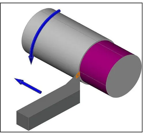
Figure 1.1: Turning Process

1.2 Problem Statement

In recent years, finite element methods (FEM) have become widely used in research and industrial applications because of the advancements in computational efficiency and speed. FEM is a useful tool for the analysis of metal cutting process where this method provide better prediction of process variables whereas interaction of the tool and the chip can also be examined.

The understanding of interactions during the cutting process is a fundamental task where this knowledge enables tool makers to evaluate the performance of the cutting tool design. Besides, it also enables the users of cutting tools to evaluate the effects of the working conditions on tool life and on the quality of the final part. Many experimental observations with trial and error are needed for the optimization of cutting conditions. Furthermore, repeating the experiment to achieved desired optimized cutting condition will be expensive and time consuming. Hence, FEM is an effective method as it would decrease experimentation and reduce cost.

In addition, much cutting force models have been developed to predict the machining parameter. Most focus mainly on dry conditions even though coolants are widely used in practical machining. Beside, research for modeling of MQL conditions is scarce and not really established. As for FEM simulation of machining, the main problem is to determine the boundary conditions at the tool-chip interface. The use of coolants in machining makes it very difficult to determine the friction coefficient at the tool-chip interface. Hence, a better understanding of friction modeling is required in order to produce more realistic finite element models of machining process. The contact behavior between the chip and the tool is critical due to its effect on the tool performance. Furthermore, the coolant method will not only affect the friction coefficient but also the heat transfer coefficient between the tool and workpiece combination.

1.3 Objective of study

The objectives of the proposed project are;

i. To study effect of various friction models, in order to predict the tool temperature and cutting force using FEM in two different conditions; dry and MQL.

ii. To investigate the effect of various heat transfer coefficient for MQL conditions.

iii. To validate the simulations results by comparing with experimental result for dry and MQL conditions.

iv. To propose the best possible friction model involved in dry and MQL turning process.

1.4 Scope of Study

The scopes of this study are:

i. Deform 2D version 9.0 software

ii. Simulation is performed in two conditions; dry and MQL iii. Cemented carbide is used as cutting tool.

iv. Workpiece material is AISI 1045

v. Experiment are running in fixed condition; Cutting speed, Vc= 160

m/min, feed, fr =0.15 mm/rev, depth of cut, d= 0.30 mm

vi. Friction model used are Coulomb, Shear, and Coulomb-Shear.

1.5 Rationale

The rationales of the present research are:

ii. FEM proved to be an efficient tool to optimize several industrial metal machining processes. The use of FEM in modeling of machining allows for considering process details that analytical models cannot handle and for predicting variables.

1.6 Overview

This study concentrates on finite element method used to simulate machining process. Simulations are running using the commercial software DEFORM 2D developed by Scientific Forming Technologies Corporation (STFC). Effects of machining parameters on cutting forces and temperature distribution are studied.

In Chapter 2, earlier experimental studies, results, and analyses reported in the literature on the topic are presented. General well known theories in metal cutting being discussed to well understand the mechanics of metal cutting. Literature on finite element analysis of machining also reviewed and discussed. Constitutive material model, material properties for these models, friction model are some of the important issues in the FEM simulation of metal cutting. Work reported in the literature addressing these issues is presented.

LITERATURE REVIEW

2.1 Introduction

2.2 Mechanics of Metal Cutting

Metal cutting is the process of removing unwanted material from the workpiece to obtain a part with high quality surfaces and accurate dimensions with acceptable tolerances. This process has represented a very large segment in industry since last century. It is estimated that 15 percent of the value of all mechanical components manufactured worldwide is derived from machining operations [4]. The metal cutting process includes different forms of machining process such as grinding, turning, milling, sawing, etc. For all these types of machining, the productions of chips have different forms and each process has unique chip morphology. Therefore, it is important to understand the mechanism of chip formation in order to understand the machining process.

In the middle of the 19th century, the old (trial and error) experimental method was the earliest way to develop models of the metal cutting process. The simplified models were also presented and used based on the shear zone theory [5]. The chip formation was assumed to take place as the result of shear actions in the shear zone. Later, finite element analysis was utilized, trying to optimize metal cutting processes. This opened a new way to investigate the state of stresses, strains, temperatures, and feed and cutting forces in the deformation zones. These models provide a better understanding of metal cutting and provided ways to do detailed studies of the effect of different parameters where the magnitude of some parameters such as the temperature cannot be easily measured experimentally.

2.2.1 Orthogonal Cutting

Figure 2.1: Orthogonal cutting geometry [6]

Figure 2.2: Oblique cutting geometry [6]

Figure 2.3: Schematic illustration of two-dimensional orthogonal cutting [7]

The uncut chip thickness (t0) is known as the feed while the deformed chip

has a different chip thickness (tc). The tool will be defined by rake angle (α) and

relief or clearance angle (β). The rake angle is defined to be positive on the right side (clockwise from vertical) and negative on the left side (counter clockwise). The contact length (lc) is defined as the distance from the tip of the tool to the point where

the chip loses contact with the tool on the rake face. The friction between the chip and the tool plays a significant role in the cutting process because of the heat energy that is transferred into the workpiece. It may be reduced by optimized tool geometry, tool material, cutting speed, rake angle, and cutting fluid. Because of the high pressure and temperature, a built up edge (BUE) may exist near the tool tip.

Figure 2.4: Thin shear plane model [6]

Once the material approaches the shear plane, the plastic deformations begins. A thin shear zone is usually created at high cutting speeds. Some researchers had different assumptions where the shear zone would be thick as shown in Figure 2.5. This kind of shear zone is more complicated and normally seen when using low cutting speeds.

Figure 2.5: Thick shear plane model [6]

2.2.2 Cutting Force in Turning

Knowing the forces that are acting in metal cutting is important for many reasons such as for the power requirement. Some parameters including the cutting speed, feed, and depth of cut influence the forces. Most likely, the forces can be reduced to two main forces in 2-D instead of three forces in 3-D.

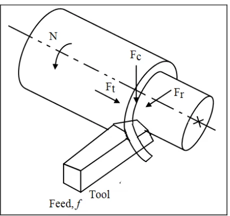
In orthogonal cutting the resultant force (Fr) applied to the chip by the tool lies in a plane normal to the tool cutting edge (Figure 2.6). This force is usually determined, in experimental work, from the measurement of two orthogonal components: one in the direction of cutting (known as cutting force Fc), the other normal to the direction of cutting (known as thrust force Ft). The cutting or tangential force (Fc), acts downward on the tool tip allowing deflection of the workpiece upward. It supplies energy required for the cutting operation. The thrust force (Ft) acts in the longitudinal direction. It is also called the feed force because it is in the feed direction of the tool. This force tends to push the tool away from the chuck.

Many researchers have correlated the measured cutting force components acting on a tool with tool wear [8] relates the wear of the cutting tool to the temperatures and measured forces acting on the tool. Force is also considered by [9] in the determination of the temperature of a machine surface. He successfully shows that the forces acting on the flank face, even with sharp tool, have been shown to be the most significant contributor to the temperatures in the workpiece.

Force modeling in metal cutting is important for thermal analysis, tool life estimation, chatter prediction, and tool condition monitoring purposes. Significant efforts have been devoted to understanding the force profiles in metal cutting. Along with a laborious experimental approach, several numerical and analytical approaches have been proposed to model the chip formation process and the associated cutting forces. Finite element method (FEM) has been applied to simulate the machining process since the early 1970s. Since then, FEM with different derivatives has received widespread attention in numerical modelling of machining processes [10]. Although some successes have been gained in modelling the chip formation forces in metal cutting by FEM, it is not yet ready to be applied due to the fact that it is laborious and not very easily extended to practical 3-D turning cases.

2.2.3 Cutting Temperature in Turning

The total work done by the cutting tool in removing metal can be determined from the values of the forces components on the cutting tool. Approximately all of this work or energy is converted into heat, which is dissipated into the tool and workpiece material; the higher the forces on the tool, the more work is needed in material removal, which in turn affects temperature. At high temperature, the cutting tool if not enough hot hard may lose their stability quickly or wear out rapidly resulting in increased cutting forces, dimensional inaccuracy of the product and shorter tool life.

of dimensional accuracy difficult and can induce thermal damage to the machined surface, adversely affecting its properties and service life.

Three regions of heat generation can be distinguished in turning; the shear zone, the chip-tool interface and the tool-workpiece interface (Figure 2.7). The primary shear zones temperatures affect the mechanical properties of the workpiece-chip material and temperatures at the tool-workpiece-chip interfaces influence tool wear.

Figure 2.7: Region of heat generation in turning [11]

Much research has been undertaken into measuring the temperatures generated during cutting operations. The main techniques used to evaluate the temperature during machining (tool-chip thermocouple, embedded thermocouple, and thermal radiation method) have been reviewed by [12] and are discussed below. Thermocouples have always been a popular transducer used in temperature measurement. Thermocouples are very rugged and inexpensive can operate over a wide temperature range. A thermocouple is created whenever two dissimilar metals touch and the contact produces a small open-circuit voltage as a function of temperature. If these two dissimilar materials are the cutting tool and the workpiece material, then this thermocouple is called a tool-chip or tool-work thermocouple.

observed. Standard thermocouples embedded in the cutting tool or workpiece material can be used to measure the temperature at a single point or at different locations to establish the temperature distribution in the tool. They can also be positioned at the interface between an indexible insert and the tool holder. Standard thermocouples are readily available at low cost and can be supplied with different types of insulation depending on the application.

Embedded thermocouples have been found to provide a good indication of the transient changes in transient changes in frictional heat generation that accompany contact area changes. Cozzens et al. [14] use many thermocouples embedded in an aluminium tube. Temperature measurements were taken at various radial and longitudinal positions in the workpiece as the tool moved down the tube. From these results, the author develops a temperature distribution model. This model then accurately predicted the peak temperatures after a coolant was used for the same cutting tests.

2.3 Minimum Quantity Lubrication (MQL)

Minimum Quantity Lubricant (MQL), also known as Near Dry Machining (NDM) or semi-dry machining, is alternative to traditional use of cutting fluids. There are many similarities between dry machining and MQL, in fact, many research papers treat that true dry machining and MQL as the same technology. As the name implies, MQL uses a very small quantity of lubricant delivered precisely to the cutting surface. Often the quantity used is so small that no lubricant is recovered from the piece. Any remaining lubricant may form a film that protects the piece from oxidation or the lubricant may vaporize completely due to the heat of the machining process. With the large volumes of cutting fluid used in traditional machining, misting, skin exposure, and fluid contamination are problems that must be addressed to assure minimal impact on worker health. With MQL, the problem of misting and skin exposure is greatly reduced, and fluid does not become contaminated because it is not re-used [15].

[16]. With this in mind, some description of lubricant performance regarding secondary characteristics is important. Because of biodegradability characteristics of synthetic ester and fatty alcohol as shown in Table 2.1:

Table 2.1: Characteristics of synthetic esters and fatty alcohol [17]

Synthetic Esters Fatty alcohols

Chemically modified vegetables oils Long-Chain alcohols made from natural raw

materials or from mineral oils

 Good biodegradability  Low level of hazard to water  Toxicologically harmless  High flash and boiling point with low

viscosity

 Very good lubrication properties  Good corrosion resistance  Inferior cooling properties  Vaporizes with residuals

 Low flash and boiling point, comparatively

high viscosity

 Poor lubrication properties

 Better heat removal due to evaporation heat  Little residuals

adopted as a replacement of dry cutting, and it may also be an alternative economic approach for flood coolant.

Wakabayashi et al. [22] also used the MQL technique in the turning process. They found that MQL provided satisfactory cutting performance compared with conventional flood coolant. Dhar et al. [23] employed MQL machining technique in turning AISI 4340 steel with uncoated carbide tool (SNMM 120408). During experimentation, process parameters such as cutting velocity, feed rate and depth of cut were kept constant at 110m/min, 0.16 mm/rev and 1.5mm respectively. Water-soluble cutting fluid was supplied at flow rate of 60 ml/h and mixed with compressed air prior to being impinged on the cutting zone at a high speed. Under same cutting conditions, MQL caused a significant reduction in tool wear and surface roughness as compared to dry and wet turning. Machado and Wallbank [24] conducted experiments on turning medium carbon steel AISI 1040 using a venture to mix compressed air (the air pressure was of 2.3 bar) with small quantities of a liquid lubricant, water soluble oil (the mean flow rate was in between 3 and 5 ml/min). The mixture was directed onto the rake face of carbide tool against the chip flow direction.

The application of mixture of air and soluble oil was able to reduce the consumption of cutting fluid, but it promoted a mist in the environment with problems of odours, bacteria and fungi growth of the overhead flooding system. For this reason, the mixture of air and water was preferred. However, even if the obtained results were encouraging, the system needed yet some development to achieve the required effects in terms of cutting forces, temperature, tool life and surface finish.

2.4 Finite Element Analysis

ABAQUS/Explicit, MARC, ALGOR, FLUENT, LS DYNA etc. Unfortunately the majority of general –purpose FEM codes are only applicable for continuous chip formation. There are specially developed FEM codes, such as DEFORM 2D, FORGE2D, AdvantEdge, which are capable of simulating segmented and discontinuous chip formation.

Ceretti [27] conducted simulation of orthogonal plane strain cutting process using FE software Deform2D. To perform this simulation with relevant accuracy, damage criteria have been used for predicting when the material starts to separate at the initiation of cutting for simulating segmented chip formation. Beside, influences of cutting parameters such as cutting speed, rake angle, and depth of cut also studied. Later, the computed cutting force, temperature, deformations and chip geometry have been compared with cutting experiments.

Halil et al. [28] compared various simulation models of orthogonal cutting process with each other as well as with the results of various experiments. Commercial implicit finite element codes MSC. Marc, Deform2D and the explicit code Thirdwave AdvantEdge have been used. In simulation with MSC. Marc and Thirdwave AdvantEdge, there is no separation criterion defined since chip formation is assumed to be due to plastic flow, therefore, the chip is formed by continuously remeshing the workpiece. However, in simulations with Deform 2D, the Cockroft-Latham damage criterion is used an elements, which exceed the predefined damage value, are erased via remeshing. Besides this different modelling of separation, the three codes also apply different friction models and material data extrapolation schemes. Estimated cutting and thrust forces, shear angles, chip thicknesses and contact lengths on the rake face by three codes are compared with experiments performed and with experimental results supplied in literature.

A new approach to carry out a coupled thermo-mechanical analysis of orthogonal cutting was proposed by [29] based on the Arbitrary Lagrangian-Eulerian formulation. Deform 2D numerical code was utilised for the plane strain simulation. The value of heat transfer coefficient is calculated through an inverse procedure, taking into account a set of experimental data and the output of the simulations.

2.4.1 Finite Element Formulation

The specific mesh formulations used for models of orthogonal machining are Lagrangian, Eulerian, and Arbitrary Lagrangian Eulerian. The Lagrangian or updated-Lagrangian method is often used in FEM. These formulations are similar. The only difference is that updated-Lagrangian uses an adaptive mesh technique to reduce mesh distortion. The updated Lagrangian formulation was first used for machining model by Klamecki [30]. The basic concept of the Lagrangian definition is that the mesh will follow the material. The deformation can happen by increments in time. After each increment the reference domain is updated based on material coordinates. In this way, the history of the material is easily taken into account. This updated position situation is used as an initial condition for the next increment, so the FE mesh is connected with its material. However, the updated-Lagrangian method can be costly because of the mesh distortion during the large deformation in these calculations (Figure 2.8).

(a) (b)

Figure 2.8: Lagrangian definition (a) Initial Mesh (b) Deformed mesh [30]

visco-plasticity, temperature, strain rate and the effect of frictional force. Marusich and Ortiz [33] presented an interesting FEM analysis of machining, based on a Lagrangian formulation with adaptive mesh processing for modelling high speed machining work. Recent work with the Updated-Lagrangian formulation was done by Ozel [34].

Another FEM option is to use the Eulerian formulation. The simple definition of the Eulerian formulation is that the mesh will be fixed in space and the material will flow through the mesh. The advantage of the Eulerian formulation is that this formulation does not have any mesh distortion because the mesh is spatially fixed during the simulation (Figure 2.9). However, the mesh does not connect to the material. It is difficult to obtain accurate data from free surfaces, which is an important result of the simulation of the forming process. Strenkowski and Moon [35] built an FEM of orthogonal metal cutting with an Eulerian formulation. The model predicted temperature distribution. He found that the shear stress occurred over a finite region in front of the tool. In the same year, Childs and Maekawa [36] used the Eulerian formulation to create an FEM to study the tool wear of cemented carbide tools in high speed machining. The results of the model were very good except there is small percentage of errors in the cutting forces.

(a) (b)

Recently, researchers have been focusing on the Arbitrary Lagrangian Eulerian (ALE) formulation to combine the best features of both the Lagrangian and Eulerian formulations. The concept of ALE was first proposed lately. This formulation was called "the coupled Eulerian-Lagrangian method" and later on was changed to "the Arbitrary Lagrangian Eulerian Model." The ALE method was introduced into the finite element method by Belytschko and Kennedy [37] .It was applied to finite strain deformation problems in solid mechanics. The ALE formulation helps to solve problems with large deformation in solid mechanics. Olovsson et al. [38] developed FEM by using the ALE formulation so that the large strain that is caused from the high deformation in metal cutting does not affect the element distortion at the tool tip. Movahhedy et al. [39] presented that the arbitrary Lagrangian- Eulerian (ALE) formulation offers the most efficient modelling approach. He included the features of an ALE analysis of the cutting process in his conclusion.

2.4.2 Modelling of Material Properties

Childs [40] stated that the success and reliability of FE based models are heavily dependent upon work material constitutive flow stress models in function of strain, strain rate and temperatures, as well as friction parameters between tool and work material interfaces. Methods to determine the flow stress data through orthogonal turning experiments were proposed by different researchers [41]. Shatla et al. [42, 43] introduced the inverse mapping of Oxley’s machining theory to determine the flow stress parameters of a modified Johnson & Cook’s equation in conjunction with orthogonal slot milling tests.

2.5 Friction Model

A general concept of friction can be considered as the tangential force generated between two surfaces. Friction can be represented as the resistance force acting on the surface to oppose slipping. Figure 2.10 (a) shows a simple example of friction where a block is pushed horizontally with mass m over rough horizontal surface. As showing in the free body diagram, Figure 2.10 (b), the body has distributions of both normal force (N) and friction force (Ff) along the contact surface. From the equilibrium, the normal force (N) acts to resist the weight force of the mass mg and the friction force (Ff) acts to resist the force F.

(a) (b)

Figure 2.10: Explanation of contact between two surfaces (a) Two bodies with friction after applying load (b) Free body diagram for the block on rough surface [6]

Basically, there are two types of friction, which are static and kinetic as shown in Figure 2.11. By increasing the force, F, friction force (Ff) increases. The blocks cannot move until the force F reaches the maximum value. This is called the limiting static fractional force. Increasing of the force F further will cause the block to begin to move. In the static portion, the limiting friction force can be expressed as:

Fstatic = µs N

Where µs is called the coefficient of static friction.

N (Ff)

mg F (2.1) F mg A B

F

(Ff) mg

F

When the force F becomes greater than Fstatic, the frictional force in the contact area drops slightly to a smaller value, which is called kinetic frictional force. Machining models generally just consider the kinetic friction coefficient which can be calculated by the following equation;

Fkinetic = µk N

Figure 2.11: Static and kinetic friction [6]

2.5.1 Friction models for machining

The attention of the researches involved in machining field was focused on friction modelling since the beginning of the studies on this process. During the time several models were proposed all over the world as summarized in the following. In the early metal cutting analysis, friction conditions at the tool-chip interface were neglected or the simple Coulomb’s law was considered on the whole contact zone, using a constant coefficient of friction µ

being the frictional stress and the normal one.

(2.2)

Another well known friction model is the constant shear model, which neglects altogether the low stress variation of with . In this case, a constant frictional stress on the rake face is assumed, equal to fixed percentage of the shear flow stress of the working material k

A more realistic model is related to the actual distribution of stresses on the rake face. The latter is rather complicated and it is typically non-linear. The normal stress decreases from the tool edge to the point where the chip separates from the tool [44]. On the contrary, the frictional stress is equal to the shear flow stress near the tool edge and then decreases. According to this distribution the existence of two distinct regions on the rake face was proposed, as shown in Figure 2.12.

Figure 2.12: Stresses distribution on rake face [44]

In the first region, named sticking zone, the normal stress is very large and the frictional stress is assumed to be equal to the shear flow stress of the material being machined. In the latter, on the contrary, the normal stress is small and Coulomb’s theory is able to provide a suitable model of the phenomenon. This can be expressed by means of the following formulation:

when

when

2.6 Conclusion

Finite element simulation of orthogonal metal cutting is become very popular nowadays and there are many research were conducted on this subject. A lot of work has been carried out to developed successful models of orthogonal metal cutting operation. A better understanding of friction modelling is required in order to produce more realistic finite element models of machining processes to support the goals of longer tool life and better surface quality. The FEM is more accurate due to ability to incorporate more realistic assumptions of material behaviour and the influence of friction. Therefore, this work is intended to compare various friction models and validate the simulation result with experimental data for two conditions; dry and MQL.

REFERENCES

1 Islam, M.N., Boswell, B., Member IAENG. An Investigation of Surface Finish in Dry Turning. Proceedings of the World Congress on Engineering. July 6-8, 2011. London, U.K.

2 Rafai, N. H., Islam, M.N., Member IAENG. Comparison of Dry and Flood Turning in Terms of Quality of Turned Parts. Proceedings of the World

Congress on Engineering. June 30-July 2, 2010. London, U.K.

3 Attanasio, A., Gelfi, M., Remino, C. (2006). Minimal quantity lubrication in turning: Effect on tool wear. Wear, 260(3), 333-338.

4 Astakhov, V.P. (2005). On the inadequacy of the single shear plane model of chip formation. International Journal of Mechanical Sciences ,47( 11),1649-1672.

5 Shaw, M. C. (1996). Metal Cutting Principles. Oxford. Oxford University Press.

6 Maftah, A. (1998). Finite Element Simulation Of Orthogonal Metal Cutting

Using An Ale Approach. University of Seventh April: Master’s Thesis.

7 Kalpakjian, S. K.(1995). Manufacturing engineering and technology.3rd ed.: Addison-Wesley Publishing.

8 Young, H.T. (1996). Cutting temperature responses to flank wear,Wear

201,117-120.

9 Chu, T., Wallbank, J. (1998). Determination of the temperature of a machined surface. J.Manuf.Sci.Eng. 2(120), 259-263.

10 E.G. Ng, Aspinwall, D.K., Brazil, D., Monaghan J. (1999). Modeling of temperature and forces when orthogonally machining hardened steel, Int. J.

11 D. O’Sullivan, M. Cotterell (2001). Temperature measurement in single point turning. Journal of Materials Processing Technology,118(3),301-308.

12 Barrow, G. (1973). Ann. CIRP, 22, 203-211.

13 Byrne, G. (1987). Thermoelectric signal characteristics and average interfacial temperature in the machining of metals under geometrically defined conditions.

Int.J.Mach.Tools Manuf., 2 (27), 215-224.

14 Cozzens, D.A.Sutherland, J.W.,Olson,W.W. (1995). An investigation into the cutting fluid effects on temperature in the aluminium boring,SME MR 95-210.

Proceedings of the First International Machining and Grinding Conference,

1995, 881-891.

15 Sharif, S.,Yusof, N.M., Idris, M.H.Ahmad, Z.A (2009). Feasibility study of using vegetable oil as a cutting lubricant through the use of minimum quauntity

lubricant during machining. Universiti Teknologi Malaysia, Department of

Manufacturing and Industrial Engineering.

16 Suda, S. Y. (2002). A Synthetic Ester as an Optimal Cutting Fluid for

Minimal Quantity Lubrication Machining. Annals of the CIRP, 51 (1), 95-98. 17 Weinert , K, Inasaki, I , Sutherland, J. W.,Wakabayashi, T. (2007). Dry

Machining and Minimum Quantity Lubrication. Annals of the CIRP,53(2),

511-537.

18 Lopez, L.N. Lamikiz, A.,Sanchez, J.A., Cabanes,I (2001). Cutting conditions and tool optimization in the high speed milling of aluminium alloys.

Proc.ImechE Part B, 215, 1257-1269.

19 Itoigawa, F., Childs.,T.H.,Nakamura,T.,Belluco,W. (2006). Effects and mechanisms in minimal quantity lubrication machining of an aluminium alloy.

Wear, 260 (3), 339-344.

20 Rahman, M., Kumar, A.S, Salam, M.U. (2001). Evaluation of minimal quantities of lubricant in end milling. Int J Adv Manuf Technol 18(4), 235-241. 21 Rahman , M, Kumar AS, Salam MU. (2002). Experimental evaluation on the

effect of minimal quantities of lubricant in milling. Int J Adv Mach Tools

Manuf , 42(5), 539-547.

23 Dhar, N.R., Kamuzzaman, M., Ahmed, M., (2006). Effect of minimum quantity lubrication (MQL) on tool wear and surface roughness in turning AISI 4340 steel.J.Mater.Process.Technol.,172, 299-304.

24 Machado, A.R., Wallbank, J.,(1997). The effect of extremely low lubricant volumes in machining. Wear, 210 (1-2), 76-82.

25 Usui, E. and Shirakashi, T. (1982). Mechanics of machining from descriptive to predictive theory, on the art of cutting metals. ASME PED ,7 , 13-35.

26 Iwata, K. (1984). Process modelling of orthogonal cutting by the rigid-plastic finite element method. Journal of Materials and Technology,106, 132-138. 27 Ceretti, E. W. (1996). Application of 2D FEM to chip formation in orthogonal

cutting. Journal of Material Processing Technology, 59, 169-180.

28 Halil, B.,Engin, K.S., Erman, T. (2004). A comparison of orthogonal cutting data from experiments with three different finite element models. International

Journal of Machine Tools & Manufacture, 44, 933-944.

29 Ceretti, E., Filice, L. (2007). ALE Simulation of Orthogonal Cutting: a New Approach to Model Heat Transfer phenomena at the Tool-Chip Interface.

Annals of the CIRP, 56(1).

30 Klamecki, B.E. (1973). Incipient chip formation in metal cutting- a three

dimension finite element analysis. Ph.D Thesis, University of Illinois,

Urbana-Champaign.

31 Carroll, J. S. (1988). Finite Element Models of Orthogonal Cutting with Application to Single Point diamond Turning. International Journal of

Mechanical Sciences, 30 (12), 889-920.

32 Shih, A.J and Yang, H.T.Y. (1993).Experimental and Finite Element Predictions of Residual Stresses due to Orthogonal Metal Cutting.

International Journal for Numerical Methods in Engineering,36, 1487-1507.

33 Marusich T. D. and Ortiz M. (1995). Modelling and Simulation of High-Speed Machining. International Journal for Numerical Methods in Engineering, 38, 3675-3694.

35 Strenkowski, J. S. and Moon, K. J (1990). Finite element prediction of chip geometry and tool/workpiece temperature distributions in orthogonal metal cutting. ASME Journal of Engineering for Industry, 112, 313-318.

36 Childs, T. H. C. and Maekawa, K. (1990).Computer-aided simulation and experimental studies of chip flow and tool wear in the turning of low alloy steels by cemented carbide tools. Wear, 139, 235-250.

37 Belytschko, T., Kennedy, J. M. (1978).Computer models for subassembly simulation. Nuclear Engineering and Design, 49, 17-38.

38 Olovsson, L., Nilsson, L. and Simonsson, K. (1999).An ALE formulation for the solution of two-dimensional metal cutting problems.Computers and

Structures,72(4), 497-507.

39 Movahhedy, M, Gadala, M.S. and Altintas, Y. (2000). Simulation of the orthogonal metal cutting process using an Arbitrary Lagrangian Eulerian finite element method. Journal of Material Processing Technology,103, 267-275. 40 Childs, T. (1998). Material Property Needs in Modeling Metal Machining. Machining Science and Technology, 2(2), 303-316.

41 Mathew, P. and Arya, N.S. (1993). Material properties from machining.

Dynamic Loading in Manufacturing and Service, 33-39.

42 Shatla, M., Kerk, C. and Altan, T. (2001). Process Modeling in Machining. Part I: Determination of Flow Stress Data. International Journal of Machine

Tools and Manufacture, 41(10), 1511-1534.

43 Shatla, M., Kerk, C. and Altan, T. (2001).Process Modeling in Machining. Part II: Validation and Applications of the Determined Flow Stress Data.

International Journal of Machine Tools and Manufacture, 41(11), 1659-1680.

44 Filice, L., Micari,F.,Rizutti, S., Umbrello, D. (2007). A critical analysis on the friction modelling in orthogonal machining. International Journal of Machine

Tools & Manufacture, 47, 709-714.

45 http://www.efunda.com/materials/alloys/carbon_steels ,accessed on 24th February.

46 Yen, Y.C., Sohner, J., Lilly, B, Altan, T. (2004) Estimation of tool wear in orthogonal cutting using finite element analysis. Journal of Material

Processing technology,146, 82-91.

48 Kops, L, Arenson, M. (1999). Convective heat transfer coefficients in turning.

In: Proceedings of the 15th Brazilian Congress of Mechanical Engineering,

Sao Paulo, Brazil.

49 Sreejith, P.S., (2008). Machining of 6061 aluminium alloy with MQL, dry and flooded lubricant conditions. Materials Letters, 62,276-278.

50 Boothroyd,G,.Knight, W.A (2006). Fundamental of Machining and machine Tools. Ohio.

51 Gouqin Shi, Xiaomin Deng, Chandrakanth Shet (2002). A finite element study of the friction in metal cutting. Finite elemet in analysis and design, 38, 863-883.

52 Shih, A.J , Chandrasekar, S.,Yang, H.T. (1990). Finite element simulation of metal cutting process with strain-rate and temperatures effects Fundamental Issues in Machining, ASME, 43, 11-24.

53 Iqbal, S.A. , Mativenga, P.T., Sheikh, M.A. (2008). A sensitivity study of the effects of interface heat transfer coefficient on FE modelling of machining process for a wide range of cutting speeds. 6th International Conference on Manufacturing Research.

54 Yen, Y.C., Sohner, J., Lilly, B., Altan, T. (2004).Estimation of tool wear in orthogonal cutting using the finite element analysis. Journal of materials