The Solution of a Coupled Nonlinear System Arising in a Three Dimensional Rotating Flow Using Spline Method

(1)

Volume 2012, Article ID 702458,12pages doi:10.1155/2012/702458

Research Article

The Solution of a Coupled Nonlinear System

Arising in a Three-Dimensional Rotating Flow

Using Spline Method

Jigisha U. Pandya

Department of Mathematics, Sarvajanik College of Engineering & Technology, Surat 395001, India

Correspondence should be addressed to Jigisha U. Pandya,[email protected]

Received 30 March 2012; Revised 28 May 2012; Accepted 26 June 2012

Academic Editor: Theodore E. Simos

Copyrightq2012 Jigisha U. Pandya. This is an open access article distributed under the Creative Commons Attribution License, which permits unrestricted use, distribution, and reproduction in any medium, provided the original work is properly cited.

The behavior of the non-linear-coupled systems arising in axially symmetric hydromagnetics flow between two horizontal plates in a rotating system is analyzed, where the lower is a stretching sheet and upper is a porous solid plate. The equations of conservation of mass and momentum are transformed to a system of coupled nonlinear ordinary diﬀerential equations. These equations for the velocity field are solved numerically by using quintic spline collocation method. To solve the nonlinear equation, quasilinearization technique has been used. The numerical results are presented through graphs, in which the eﬀects of viscosity, through flow, magnetic flux, and rotational velocity on velocity field are discussed.

1. Introduction

In fluid mechanics, the problems associated with the flow that occurs due to the rotation of a single disk or that between two rotating disks have been found of interest of many researchers. Flows between finite disks were studied by Dijkstra and van Heijst1, Adams and Szeri2and Szeri et al.3. Berker4showed that when the two disks are rotating with the same angular speed, there exists a one parameter family of solutions all but one of which is not rotationally symmetric. This result has been extended by Parter and Rajagopal 5, to disks rotating with diﬀering angular speeds; they prove that the rotationally symmetric solutions are never isolated when considered within the full scope of the Navier-Stokes equations. The numerical study of the asymmetric flow has been carried out by Lai et al. 6,7.

(2)

sheet at a diﬀerent uniform temperature. Banerjee 9studied the eﬀect of rotation on the hydromagnetic flow between two parallel plates where the upper plate is porous and solid, and the lower plate is a stretching sheet.

In this paper, we analyze the behavior of the solution of the nonlinear coupled systems arising in axially symmetric hydromagnetic flow between two horizontal plates in a rotating system, where the lower plate is a stretching sheet. The governing coupled ordinary diﬀerential equations are solved by quintic spline collocation method.

InSection 2, the mathematical model of the problem given by Vajravelu and Kumar 10is presented. The quintic spline collocation method is explained inSection 3. The results are displayed in graphical manner in Section 4, and the discussion of results is drawn in

Section 5.

2. Formulation of the Problem

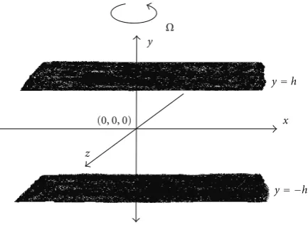
We consider the steady flow of an electrically conducting fluid between two horizontal parallel plates when the fluid and the plates rotate in unison about an axis normal to the plates with an angular velocityΩ. A Cartesian coordinate system is considered in such a way that thex-axis is along the plate, they-axis is perpendicular to it, and thez-axis is normal to thexy-plane as shown inFigure 1.

The origin is located at the centre of the channel, and the plates are located aty−h

andh. The lower plate is is stretched by introducing two equal and opposite forces so that the position of the point0,−h,0remains unchanged. A uniform magnetic flux with density

Bois acting alongy-axis about which the system is rotating. The upper plate is subjected to

a constant wall injection with a velocityVo. The equations of motion in a rotating frame of

reference are

u∂u

∂x υ

∂u

∂y 2Ωω−

1

ρ ∂p∗

∂x ν

∂2_u

∂x2

∂2_u

∂y2

−σBo2

ρ u, 2.1

u∂υ

∂y −

1

ρ ∂p∗

∂y ν

∂2υ ∂x2

∂2υ ∂y2

, 2.2

u∂ω

∂x υ

∂ω

∂y −2Ωuν

∂2_ω

∂x2

∂2_ω

∂y2

−σBo2

ρ ω, 2.3

∂u ∂x

∂υ

∂y 0, 2.4

whereu, υ, andω denote the fluid velocity components along thex, y, andzdirections,ν

is the kinematics coeﬃcient of viscosity,ρis the fluid density, andp∗ is the modified fluid pressure. The velocity is independent ofzand that all derivatives towardsztherefore do not appear in the equations of motion. This leads to the absence of∂p∗/∂zin2.3which implies that there is a net cross-flow along thez-axis.

The boundary conditions are

uEx, υ0, ω0 aty−h,

u0, υ−υ0, ω0 atyh.

(3)

y

z

x Ω

(0, 0, 0)

y=h

[image:3.600.193.410.97.262.2]

y= −h

Figure 1: Flow configuration.

We introduce nondimensional variables

η y

h, uExf

_η_, _υ₋_Ehf_η_, _ω_Exg_η_, _2.6

where a prime denotes diﬀerentiation with respect toη. Substituting2.6in2.1to2.4, we have

−1 ρ

∂p∗

∂x E

2_x

f2−ff−f

R M2

R f

2K2

R g

, 2.7

− 1 ρh

∂p∗

∂η E

2_h

ff 1

Rf

_, _2.8

g−Rfg−fg 2K2f−M2g 0, 2.9

where

R Eh

2

ν , viscosity parameter,

M2 σB

2

0h2

ρν , magnetic parameter,

K2 Ωh

2

ν , the rotation parameter.

2.10

Equation2.7with the help of2.8can be written as

f−Rf2−ff−2K2g−M2fA, 2.11

(4)

Diﬀerentiation of2.11with respect toηgives

f−Rff−ff−2K2g−M2f0. 2.12

Thus we solve the following nonlinear system numerically for several sets of values of the parameters:

f−Rff−ff−2K2g−M2f0,

g−Rfg−fg 2k2_f₋_M2_g ₀_, 2.13

subject to the boundary conditions

f0, f1, g0 atη−1,

fλ, f0, g0 atη1, 2.14

whereλυ0/Eha parameter depending on the y component of velocity at the upper plate.

3. Quintic Spline Collocation Method

The fifth degree spline is used to find numerical solutions to the boundary value problems discussed in2.13together with2.14. A detailed description of spline functions generated by subdivision is given by de Boor11.

Consider equally spaced knots of a partitionπ:a xo < x1 < x2 < · · · < xn bon

a, b. LetS5πbe the space of continuously diﬀerentiable, piecewise, Quintic polynomials

onπ. That is,S5πis the space of Quintic polynomials onπ. The Quintic spline is given by

Bickley12and by G. Micula and S. Micula13

sxa0 b0x−x0

1

2 c0x−x0

2 1

6d0x−x0

3 1

24e0x−x0

4 1

120

n−1

k0

Fkx−xk5, 3.1

where the power functionx−xk is defined as

x−xk

x−xk, ifx > xk,

0, ifx≤xk,

3.2

Consider a fourth-order linear boundary value problem of the form

(5)

α0y0 β0yn γ0yn δ0ynη0,

α3y0 β3 yn γ3yn δ3ynη3,

3.4

whereyx, px, qx, rx, tx, andmxare continuous functions defined in the interval

x∈a, b; η0, η1, η2, η3are finite real constants.

Let3.1be an approximate solution of3.3, wherea0,b0,c0,d0,e0,F0,F1, . . . , Fn−1are

real coeﬃcients to be determined.

Letx0, x1, . . . , xnben 1 grid points in the intervala, b, so that

xia ih, i0,1, . . . n; x0a, xnb, h

b−a

n . 3.5

It is required that the approximate solution 3.1 satisfies the diﬀerential equation at the pointx xi. Putting3.1with its successive derivatives in3.3, we obtain the collocation

equations as follows:

n−1

k0

Fk

xi−xk

1

2pxixi−xk

2 1

6qxixi−xk

3 1

24rxixi−xk

4

1

120txixi−xk

5

e0

1 pxixi−x0

1

2qxixi−x0

2 1

6rxixi−x0

3 1

24txixi−x0

4

d0

pxi qxixi−x0 1

2rxixi−x0

2 1

6txixi−x0

3

c0

qxi rxixi−x0

1

2txixi−x0

2

b0{rxi txixi−x0} a0{txi}

mxi, i0,1,2, . . . , n.

3.6

From boundary conditions,

n−1

k0

Fk

δ0

2 b−xk

2 γ0

6b−xk

3 _e

0

δ0b−a

γ0

2b−a

2

d0

δ0 γ0b−a

c0

γ0

b0

β0

(6)

n−1 k0 Fk δ1

2 b−xk

2 γ1

6b−xk

3 β1

120b−xk

5

e0

δ1b−a

γ1

2b−a

2 β1

24b−a

4

d0

δ1 γ1b−a

β1

6b−a

3 c0 γ1 β1

2b−a

2

b0

β1b−a α1

a0

β1

η1,

n−1

k0

Fk

δ2

2 b−xk

2 γ2

6b−xk

3 β2

120b−xk

5

e0

δ2b−a

γ2

2b−a

2 β2

24b−a

4

d0

δ2 γ2b−a

β2

6b−a

3 c0 γ2 β2

2b−a

2 _γ

2b−a α2

b0

β2b−a

a0

β2

η2,

n−1

k0

Fk

δ3

2 b−xk

2 γ3

6b−xk

3 β3

120b−xk

5

e0

δ3b−a

γ3

2b−a

2 β3

24b−a

4

d0

δ3 γ3b−a

β3

6b−a

3 _α 3 c0 γ3 β3

2b−a

2

b0

β3b−a

a0

β3

η3.

3.7

Using the power functionx−xk in the above equations, a system ofn 5 linear equations

inn 5 unknownsa0,b0,c0,d0,e0,F0,F1, . . . , Fn−1is thus obtained. This system can be written

in matrix-vector form as follows:

AX B, 3.8

where X Fn−1, Fn−2, . . . , F2, F1, F0, e0, d0, c0, b0, a0T,B η3, η2, η1, η0, mxn,

mxn−1, . . . , mx1,mx0T.

The coeﬃcient matrixAis an upper triangular Hessenberg matrix with a single lower subdiagonal, principal and upper diagonal having nonzero elements. Because of this nature of matrixA, the determination of the required quantities becomes simple and consumes less time. The values of these constants ultimately yield the quintic splinesxin3.1.

(7)

with fitting a curve satisfying the end conditions and this curve is designated asyi. We obtain

the successive iterations yi’s with the help of an algorithm described as above till desired

accuracy.

4. Quintic Spline Solution

We solve following nonlinear system numerically for several sets of values of the parameters:

f−Rff−ff−2K2_g₋_M2_f₀_, _4.1

g−Rfg−fg 2K2f−M2g 0. 4.2

f0, f1, g0 atη−1,

fλ, f0, g0 atη1. 4.3

The spline collocation method is used to solve the diﬀerentiation system4.1to4.3. Equation4.2is a linear equation of order two, whereas4.1is a nonlinear equation of order four. For solving nonlinear equation by spline collocation method, we require a linear form of diﬀerentiation equation. The quasilinearization technique transforms4.1into linearized form as

f_iiv₁ Rfi

f_i₁−Rfi M2

f_i₁−Rf_if_i₁ Rf_ifi 1 2K2gi R

fifi −fifi

, 4.4

with boundary conditions

fi 1−1 0, fi 1−1 1,

fi 11 λ, fi 11 0.

4.5

The linear equation4.2can be written as

g Rfg−Rf M2g−2K2f 4.6

with boundary conditions

g−1 0, g1 0. 4.7

(8)

The quintic spline given by

sηi

a0 b0

ηi−η0

1

2c0

ηi−η0

2 1

6d0

ηi−η0

3 1

24e0

ηi−η0

4 1

120

n−1

k0

Fk

ηi−ηk

5

4.8

is an approximate solution of the problem given by4.4and4.5. Substitutingsηin both of above equations, we obtain the collocation as

N−1

k0

Fk

ηi−ηk

Rfi

2

ηi−ηk

2 ₋

Rf_i M2

6

ηi−ηk

3

−Rfi

2

ηi−ηk

4 Rf

120

ηi−ηk

5

e0

1 Rfi

ηi−η0

−

Rf_i M2

2

ηi−η0

2₋Rfi

6

ηi−η0

3 Rfi

24

ηi−η0

4

d0

Rfi−

Rf_i M2ηi−η0

−Rfi

2

ηi−η0

2 Rfi

6

ηi−η0

3

c0

−Rf_i M2−Rf_iηi−η0

Rf_i

2

ηi−η0

2

b0

Rf_iηi−η0

−Rf_i a0

Rf_i 2K2g_i Rfifi fifi

, i01N.

4.9

First two boundary conditions in4.5immediately give

a00, b01, 4.10

and other two boundary conditions are

1 120

N−1

k0

Fk

ηN−ηk

5 1

24e0

ηN−η0

4 1

6d0

ηN−η0

3

1 2c0

ηN−η0 2

b0

ηN−η0

a0 λ,

1 24

N−1

k0

Fk

ηN−ηk

5 1

6e0

ηN−η0

3 1

2d0

ηN−η0 2

c0

ηN−η0

b00.

(9)

0 1 2 3 4

I II III

IV V

I II III IV V

1 1 1 3 3

1 1 3 3 3

0 3 3 3 25

−1.5

−1

−0.5

0 0.5 1 1.5

f =v/−Eh

η

=

y/

h

λ

M2

[image:9.600.185.416.98.389.2]

K2

Figure 2: Velocity profile forR0.1, N10.

First of all, initial assumptions regardingfi, f_i, f_i, f_iare necessary. Let a curveaη3 bη2 cη d

be fitted through the pointsη −1 andη 1 satisfying the boundary conditions4.5. This requirement yieldsa 1−λ/4, b −1/4, c 3λ −1/4 andd 1 2λ/4 so that

fη 1−λ/4η3₋₁_/₄_η2₃_λ₋₁_/₄_η₁ ₂_λ_/₄_.

Further, using the cubic spline

sηi

a0 b0

ηi−η0

1

2c0

ηi−η0

2 1

6

n−1

k0

dk

ηi−η0

3

. 4.12

In4.6and4.7, the following set of equations is obtained:

N−1

k0

dk

ηi−ηk

0.1fi

2

ηi−ηk

2₋

0.1f_i 1 6

ηi−ηk

3

c0

1 0.1fi

ηi−η0

−

0.1f_i 1 2

ni−η0

2

b0

0.1fi−

0.1f_i 1ηi−η0 a0

−0.1f_i 1

−2K2f_i, i01N,

a00

(10)

0 1 2 3

I II III

IV V

I II III IV V

1 1 1 3 3

1 1 3 3 3

0 3 3 3 25

f₌_u/Ex

−1.5

−1

−0.5

0 0.5 1 1.5

η

=

y/

h

λ

M2

[image:10.600.185.416.94.377.2]

K2

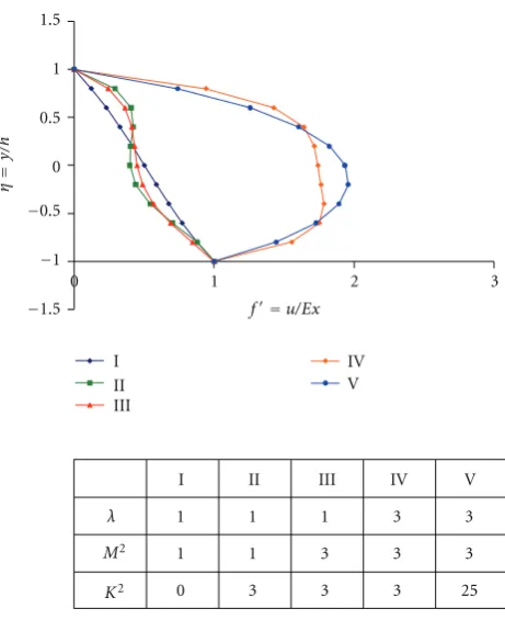
Figure 3: Velocity profile forfR0.1, N10.

and the last equation is

1 6

N−1

k0

dk

ηN−ηk

3 1

2c0

ηN−η0

2

b0

ηN−η0

a00. 4.14

A straight linegη aη bcan be fitted to the boundary conditions forg. A line

gη 0 satisfied the boundary conditions4.7. Therefore, initial values ofg andgare also zero.

ForN 10,R 0.1 and several sets of values of the parametersλ, M2 _and_K2_{, the}

velocity componentsf, f, and g are obtained in graphical form. The behavior of velocity components are shown in Figures2,3, and4. The results obtained by the spline collocation method are compared with the graphical solutions obtained by Vajravelu and Kumar10, which are tested by comparing the analytical solutions for small value of R with the exact solutionsf andg. The numerical results thus obtained by the spline method to find

f, f, andg are in close agreement with the available data. In Figures2,3, and4,η equals a dimensionless injection parameter, M2 _{is a magnetic parameter, and} _K2 _{is a rotational}

parameter.

(11)

−1 9 19 29

I II III

IV V

I II III IV V

1 1 1 3 3

1 1 3 3 3

0 3 3 3 25

−1.5 −1 −0.5 0 0.5 1 1.5

η

=

y/

h

g=ω/Ex

λ

M2

[image:11.600.184.415.99.398.2]

K2

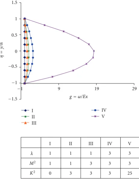
Figure 4: Velocity profile forgR0.1,N10.

5. Discussion of the Results

The behavior of the nondimensional velocity componentfforR 0.1 is shown inFigure 2. From Figure 2, it is evident that the Lorenz force decreases the velocity componentf see curves II and III, but the value off increases with an increase in the value of the parameter

λas seen in curves III and IV. Further, inFigure 2, curves IV and V show thatf decreases steadily for smallK2_{, whereas for large value of} _K2_{, f increases near the lower plate and}

decreases near the upper plate.

Figure 3 describes the behavior of fη, which is proportional to velocity along parallel plates, for several sets of values of the parameters onlyλ, M2_and_K2 _{the rotation}

parameterare varied whileRis kept constant at 0.1. FromFigure 3, curves III and IV, it is evident that the velocity componentfincreases with the parameterλυ0/Eh,ycomponent

of velocity at the upper plate, and the increase is maximized near the stretching plate. However, the eﬀect of the Lorenz forcemagnetic parameterM2_of_f_{is to increase it near}

the upper plate and to decrease it near the lowerstretchingplate that is displayed from the curves II and III ofFigure 3. Further, the eﬀect of smallK2_{is to increase}_f_{at the upper plate} and to decrease it near the lower plate is evident from curves I and II. But the eﬀect of large

K2 _{is to increase}_f_{near the plates and to decrease it at the centre of the channel. Also, the} rotation of the channel brings humps near the plates, indicating the occurrence of a boundary layer near the plates. Furthermore, for largeK2_{the coriolis force and the magnetic field that}

(12)

The transverse velocityg increases as the parameterλ increases, which is shown in curves III and IV ofFigure 4. But this is quite opposite to the phenomenon with the magnetic parameterM2_{. However, the rotation parameter}_K2_increases_g_{and the maximum of}_g_occurs

near the stretching sheet for largeK2_.

From above figures, it is observed that for largeK2convergence in the results is not guaranteed. This fact is also observed by Vajravelu and Kumar10.

We conclude from the above numerical experience that the spline collocation method can be successfully applied to solve the fourth-order nonlinear coupled equation, which governs the hydromagnetic fluid flow. This widens the field of applicability to the higher-order coupled diﬀerential equations. This encourages the applications to other types of problems.

Another useful conclusion is that the selection of the domain is not restricted to positive interval only. That is we can successfully apply the above method for the negative intervals as the domain of the problem.

References

1 D. Dijkstra and G. J. F. van Heijst, “Flow between two finite rotating disks enclosed by a cylinder,”

Journal of Fluid Mechanics, vol. 128, pp. 123–154, 1983.

2 M. L. Adams and A. Z. Szeri, “Incompressible flow between finite disks,” Journal of Applied Mechanics,

Transactions ASME, vol. 49, no. 1, pp. 1–9, 1982.

3 A. Z. Szeri, S. J. Schneider, F. Labbe, and H. N. Kaufman, “Flow between rotating disks—part 1. Basic flow,” The Journal of Fluid Mechanics, vol. 134, p. 103, 1983.

4 R. Berker, “A new solution of the Navier-Stokes equation for the motion of a fluid contained between two parallel plates rotating about the same axis,” Archives of Mechanics, vol. 31, no. 2, pp. 265–280, 1979.

5 S. V. Parter and K. R. Rajagopal, “Swirling flow between rotating plates,” Archive for Rational Mechanics

and Analysis, vol. 86, no. 4, pp. 305–315, 1984.

6 C. Y. Lai, K. R. Rajagopal, and A. Z. Szeri, “Asymmetric flow between parallel rotating disks,” The

Journal of Fluid Mechanics, vol. 146, p. 203, 1984.

7 C. Y. Lai, K. R. Rajagopal, and A. Z. Szeri, “Asymmetric flow above a rotating disk,” Journal of Fluid

Mechanics, vol. 157, pp. 471–492, 1985.

8 A. Chakrabarti and A. S. Gupta, “Hydromagnetic flow and heat transfer over a stretching sheet,”

Quarterly of Applied Mathematics, vol. 37, no. 1, pp. 73–78, 1979.

9 B. Banerjee, “Magnetohydrodynamic flow between two horizontal plates in a rotating system, the lower plate being a stretched sheet,” Journal of Applied Mechanics, Transactions ASME, vol. 50, p. 470, 1983.

10 K. Vajravelu and B. V. R. Kumar, “Analytical and numerical solutions of a coupled non-linear system arising in a three-dimensional rotating flow,” International Journal of Non-Linear Mechanics, vol. 39, pp. 13–24, 2004.

11 C. de Boor, A Practical Guide to Splines, vol. 27, Springer, New York, NY, USA, 1978.

12 W. G. Bickley, “Piecewise cubic interpolation and two-point boundary problems,” The Computer

Journal, vol. 11, pp. 206–208, 1968.

13 G. Micula and S. Micula, Handbook of splines, Kluwer Academic Publishers, Dordrecht, The Netherlands, 1998.

(13)

Submit your manuscripts at

http://www.hindawi.com

Hindawi Publishing Corporation

http://www.hindawi.com Volume 2014

Mathematics

Journal of

Hindawi Publishing Corporation http://www.hindawi.com

Differential Equations

International Journal of

Volume 2014

Applied MathematicsJournal of

Mathematical PhysicsAdvances in

Complex Analysis

Journal of

Optimization

Journal of Hindawi Publishing Corporation

Combinatorics

International Journal of

Journal of

Function Spaces

Abstract and Applied Analysis Hindawi Publishing Corporation

International Journal of Mathematics and Mathematical Sciences

Hindawi Publishing Corporation http://www.hindawi.com Volume 2014

The Scientific

World Journal

Discrete Dynamics in Nature and Society

Discrete Mathematics

Journal of

The Solution of a Coupled Nonlinear System Arising in a Three Dimensional Rotating Flow Using Spline Method

Research Article