251
APPLICATION OF NESTED COST OPTIMIZATION MODELS
TO TSPD
1XIA WEN- HUI, 2LIU JUAN-HONG, 3ZENG HONG
1,2 School of Business Administration, Chongqing University of Technology, China, 400054
3
School of Metallurgical Engineerning, Chongqing University of Science and Technology, China, 401331
E-mail: [email protected] , [email protected] , [email protected]
ABSTRACT
Through the analysis of Travelling Salesman Problem with Pickup and Delivery (TSPD) in the related research, two kinds of logistics systems including whole logistics system and partial logistics system under one-to-many logistic network are considered. And mathematical model is set up, then, nested cost optimization model is set up in order to meet the constraint condition of nested order cycle time. According to an application pickup and delivery instance of iron and steel in one factory, by using the method of adaptive response surface in Hyperstudy software, the initial solutions are figured out, and further the optimum direction of iteration is found so as to obtain the optimum solution.
Keywords: Nested, Logistics System, Pickup and Delivery, Cost models, Optimal Solution
1. INTRODUCTION
System integrated and cost optimization are considered, which complement each other, are the integral goal of modern logistics distribution system. And cost control is the most important procedure for optimizing the system. In fact, the cost mainly comes from transport and inventory, which take the main parts. So to integrate Vehicle Routing Problem and inventory control is the key point of the researching on this paper. The research purpose is minimizing the sum of cost through optimizing and controlling the different types of costs respectively.
In the course of planning and operating logistics distribution system, Travelling Salesman Problem with Pickup and Delivery(TSPD), which is characterized by a set of customers, each of them supplying (pickup customer) or demanding (delivery customer) a given amount of product[1], usually occurs. And it is affected by many factor, this article only considers both the demand of pickup and delivery for logistics distribution system and the most loading of vehicles. Therefore, it is not allowed to neglect to the influence of the collection cost. TSPD is actually an NP-hard problem, so the related researches focus on algorithm. About simultaneous pickup and delivery, a heuristic solution approach based on particle swarm optimization is presented [2]. The problem and LIFO loading by considering the use of multiple
vehicles and a limitation on the total distance is extended by Cheang B [3]. And a variable neighborhood search approach is showed by Mladenovic N [4]. Besides, scholars have researched some solutions of TSPD by genetic algorithm [5]-[6], ant colony algorithm [7]-[8] and so on. Nested viewpoint [9] and adaptive response surface algorithm is combined in order to get a better solution.
In this paper whole logistics system and partial logistics system under one-to-many logistic
network are described. Then, nested cost
optimization models that meets the constraints of nested order cycle time are set up. At last, a related analysis and calculation is carried out by taking the delivery and pickup of an iron and steel company as a case.
2. MODELING
This paper researches the one-to-many logistics delivery system, which is defined as one DC supplies goods for many retailers. The proposition sets for the distribution goods is single.
Firstly, the application of model to real-life problems is governed by the following design guidelines:
252 that a part of customers delivery demand is not less than the pickup demand, others is not more than the pickup demand.
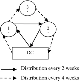
[image:2.612.106.238.243.382.2]2) Nested order cycle time is the order cycle of one or more retailers that is nested another order cycle to reduce delivery costs. Furthermore, they are satisfied the rule of the second power. For example, the order cycle of the retailer One and Two is 2, means the nested cycle time. The retailer Three having nested order cycle time, means the nestable cycle time, is 4. The sketch map is shown in Figure 1.
Figure 1 Nested Order Cycle TimeDistribution Sketch Map
Secondly, the assumptions to build the model are used as follows:
①Transportation cost considers the start-up cost
of vehicles but not vehicle traffic lines. And the order cost is not contained because of all order operations are carried out under the e-commerce platform.
②All retailers have the inventory and the supply
of inventory meets the order cycle.
③The DC has pickup areas, and the capacity is
Q. It is less than the total capacity of the pickup demand of all customers.
④Each distribution generates inventory cost.
⑤Each retailer makes sure the distribution
number independently, and the number reaches the capacity of retailers.
⑥The pickup activities generate the cost, which
is only related to the pickup number.
Finally, the symbols used in the model are described as follows:
Where i= {1,2, ..., N} is a retailer set ,with N being the number of all the retailers .and smaller one has shorter order cycle. The DC is i = 0. The
delivery demand of the retailer i is di. The pickup
demand of retailer i is pi ; The unit inventory cost
of the retailer i is gi. . The unit pickup cost of the
retailer i is wi. The order cycle is Ti.
The objective function is to seek the optimal nested order cycle time which can get a minimum cost including of delivery cost, inventory cost and pickup cost. The paper assumes that the capacity of all vehicles in the DC is the same as R .And the DC supplies service for n customers having delivery and pickup demand. So the lest number of vehicles
is .In
this logistics system, the number of vehicles is H, they provide service for all the retailers. So
.
Where Ph is the running route of vehicle h, L (1)
is an initial capacity of the vehicle. ih is the current
point when the vehicle h runs along Ph, cd(ih) is the
cumulative delivery demand along Ph , cp(ih) is the
cumulative pickup demand along Ph. This paper
indicates di≥pi (i=2,3…n) in whole logistics
system ,but di≥0,pi≥0 in partial logistics system.
2.1 COST CALCULATION
A customer follows nested order cycle time ,
which is satisfied the rule of the second power, and
T1≤T2≤…≤Tn. Furthermore, smaller customers
have shorter order cycle time.So, the distribution
routes include{1},{1,2},…,{1,2,…,i},…,
{1,2,…,n}. This paper presents a method of expressing the transportation cost of {1,2,…,i} by
M({1,2,…,i}),and fi= M({1,2,…,i}).So the
calculation formula of transportation cost in the
whole logistics system is [M({1,2,…,i})
-M({1,2,…,(i-1)})]Ti-1= (f i - fi-1)Ti-1.
In partial logistics system, the most loading of customers is denoted L(ih) = L(1)-cd(ih)+ cp(ih). It is maybe greater than the one of vehicles.Therefore the TSPD in existence should be improved. In the DC, the vehicles must be started regardless of the number of the order goods, and the start-up cost is regarded as the fixed one. The model of transportation cost from these customers is presented as follows:
fi= min (cklzkl +c0h)
subject to L(ih) ≤R, DC
2
1
11
31
Distribution every 2 weeks
253 zkl≤1(k=1,2,…,n),
zkl≤1(l=1,2,…,n),
zkl∈{ 0,1 } ((k,l=1,2,…,n).
Where co is the average startup cost. ckl is the
distance between k and l.zkl is the number of
passing through ckl, and it is 1 if passing otherwise
is 0.Then, (f i - fi-1)Ti-1 denotes the total cost of
transportation in the planning.
If each customer meets the condition of L(ih) ≤R
,this route is the best. digiTi/2 expresses the
total cost of inventory taking no account of the cost
of DC. And wi piTi is the total cost of pickup.
2.2 INITIAL MODEL
Based on the above analysis, the problem can be formulated as:
min[F(T)] = (f i - fi-1)Ti-1 + digiTi/2+
wi piTi
subject to 0 <T1≤T2≤…≤Tn(i= 1,2,…,n)
(1)
Ti= (m is a integer, Unit period is 1 )
(2)
diTi≤hR (i= 1,2,…,n)
(3)
piTi ≥ Q
(4)
0≤p≤ di Or 0≤pi , 0≤ di.
(5)
Where the objective minimizes the total cost of transportation, inventory and pickup, nested order cycle time is ensured by(1)-(2), the capacity of vehicles is enforced by(3), the capacity of pickup area in DC is ensured by(4) and the demand of
pickup meets constraint (5),but it is 0≤p≤ di in the
whole logistics system , while 0≤pi,0≤ di in the
partial logistics system.
2.3 NESTED COST OPTIMIZATION MODEL
For the finally optimal solution T*, it does not
necessarily satisfy the nested constraint. So the new model is set up in order to solve this problem and
defined as nested cost optimization model, as follows:
min[F(T*)] = (f i - fi-1)Ti -1
+ digiTi/2+
wi piTi
subject to Tio=2k-1,Tiu=2k(k is a integer,2k-1≤Ti
*
≤2k)
diTi≤hR (i= 1,2,…,n),
piTi≥Q,
0≤pi≤di.
Where 2k-1≤T*≤2k, and k is an integer. And
Tio=2k-1, Tiu=2k.
3. EXPERIMENTATION
The paper takes the delivery and pickup of an iron and steel company (in Chongqing) as the experimentation.
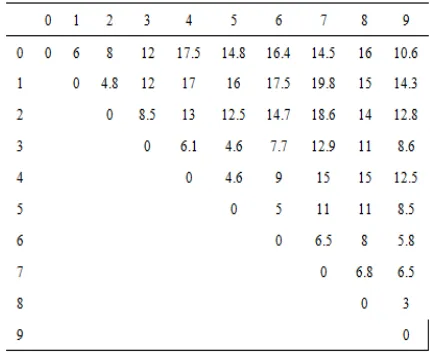
[image:3.612.325.540.405.585.2]Table 1 The Vehicle Operating Cost Of Each Customer (Unit:RMB)
Table 2 The Delivery And Pickup Demand In Whole Logistics System
Unit:di and pi is kg each unit time, gi is RMB
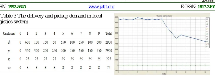
254 Table 3 The delivery and pickup demand in local logistics system
Unit is just the same as Table 3.
The company has a DC to serve 9 customers with TSPD. The vehicle operating cost of each customer is shown as Table 1, and 0 is DC. The delivery and pickup demand in whole logistics system and local logistics system is given in Table 2 and Table 3 below.
Where the capacity of vehicle is 1000 kg, the least vehicle number is 3. The average start-up cost is 10 RMB. The pickup capacity of DC is 2000 kg, and the unit order cycle is 1 week.
3.1 WHOLE LOGISTICS SYSTEM OPTIMIZATION
According to Table1and Table 2, the whole logistics system model is given as follows:
min[F(T)] = (f i - fi-1)Ti -1
+ digiTi/2+
wi piTi
subject to 0 <T1≤T2≤…≤T9
600T1+100T2+150T3+50T4+650T5+10
0T6+550T7+100T8+600T9≤3000
600T1+100T2+150T3+50T4+650T5+100T
6+550T7+100T8+600T9≥2000
0≤pi=di ,(i= 1,2,…,n)
The paper applies the method of adaptive response surface in Hyperstudy software to optimize the problem.
Figure 2 The Iterative Process Of Whole Logistics System
After 20 iterations, the optimum solution is obtained. The iterative process is shown in Figure 2.
Due to limited space available, this paper only
shows the result.
So, T =(T1,T2,…T9)=(0.02,0.02,0.02,0.02,
0.53,1.21,1.21,1.21,1.21),The target value is min
[f (T)] = 42717.8 RMB. The solution does not meet the nested constraint condition. Therefore, nested cost optimization calculation should be continued. There are
2-3≤T1=T2=T3= T4≤2-2,
2-1≤T5≤1,
1≤T6= T7=T8= T9≤2.
So each order cycle may have two values,
T1= T2=T3= T4= {2 -3,
2-2},
T5={2-1,1},
T6= T7=T8= T9={1,2}.
The whole solutions are 29, with T* being the
optimum solution. The meaning of the objective function is the minimum cost meeting the nested
constraint. So T*is found, just as{0.125,0.125,
0.125, 0.125,1,1,1,1,1}, the target value is
min[F(T*) ]=46610.3 RMB.
3.2 LOCAL LOGISTICS SYSTEM OPTIMIZATION
Similarly, the initial optimal solution in local logistics system is T=
(0.52,0.52,0.52,0.52,0.77,0.77,0.77,0.77,0.77 ).
And the corresponding target value is
min[F(T)]=40693.9 RMB.
255
Figure 3 The Iterative Process Of Partial Logistics System
The optimal solution is get ,
T*={0.5, 0.5, 0.5, 0.5, 0.5, 0.5, 1, 1, 1}.
And the target value is
min[F ( T * ) ]=43023.8 RMB.
4. CONCLUSION
Based on the paper—cost Optimization Models of Nested Sequence Policy Under the One-to-Many Pickup and Delivery System—which is wrote by Xu Jiu-ping and Lei Zhen, this paper takes transportation, inventory and pickup as a whole after analyzing TSPD and introducing related work recently. Nested cost optimization model is set up respectively according to the different between whole logistics system and partial logistics system. The study explores the new algorithm combining with the experimentation about two kinds of logistics system and gains the solution. So as to reveal application of the nested cost optimization model to TSPD.
REFRENCES:
[1] H Hipólito., et al. A Hybrid GRASP/VND Heuristic for the One-commodity Pickup-and-delivery Traveling Salesman Problem.
Computers & Operations Research. pp.
1639-1645.May 2009.
[2] F.P Goksala, I Karaoglanb, Hybrid Discrete Particle Swarm Optimization for Vehicle Routing Problem with Simultaneous Pickup and
Delivery. Computers & Industrial Engineering.
Jan 2012.
[3] B Cheang , et al .Multiple Pickup and Delivery Traveling Salesman Problem with
Last-in-first-out Loading and Distance Constraints.
European Journal of Operational Research.
Vol 1(223), pp.60–75 Nov 2012.
[4] N Mladenovic, et al. A General Variable Neighborhood Search for the One-commodity
Pickup-and-delivery Travelling Salesman
Problem. European Journal of Operational
Research.Vol 220 (1), pp.270-285. 2012.
[5] V Çınar, T Öncan and H Süral.A Genetic
Algorithm for the Traveling Salesman Problem with Pickup and Delivery Using Depot
Removal and Insertion Moves.Applications of
Evolutionary Computation,pp.431-440,2010.
[6] N. Velasco, P. Dejax, C. Guéret & C. Prins。A
Non-dominated Sorting Genetic Algorithm for a Bi-objective Pickup and Delivery Problem.
Engineering Optimization. Issue 3, pp. 305-325.
2012.
[7] R Falcon, et al. The One-Commodity Traveling Salesman Problem with Selective Pickup and
Delivery: an Ant Colony Approach.
Evolutionary Computation (CEC), pp. 1 – 8,Jul
2010.
[8] E John. et al .Swarm Intelligence : Application of Ant Colony Optimization Algorithm to Logistics-oriented Vehicle Routing Problems.
Journal of Business Logistics. Vol 2(31) , pp,
157–175, 2010.
[9] Xu Jiuping, Lei Zhen .Cost Optimization Models of Nested Sequence Policy Under the
One-to-Many Pickup and Delivery System. Chinese