3832
Optimization of Micro-hardness of Al-SiC 6061 MMC
Machined by Wire EDM with Taguchi method.
Rohit Sharma
1, Vivek Aggarwal
2, H. S. Payal
3Mechanical Engineering1,2,3, IKGPTU, Kapurthala1,2, Himalayan School of Engineering and Technology,
Dehradun3
Email: [email protected]om1, [email protected], payal_hs@yahoo.com3
Abstract-The usage of Al-SiC metal matrix composites is constantly increasing since the last many years due to their many unique properties such as light weight, high strength, high specific modulus, high fatigue strength, low density, and high hardness. However, because of their high hardness, their machining, that too within close tolerance limits, is often a big challenge. Wire EDM machining however offers a good method to machine these deemed difficult to machine alloys. This research work focuses on the wire EDM machining of Al-SiC 6061 metal matrix composite which is one of the most widely used metal matrix composites in the world today. Here, Taguchi approach has been applied to study the work-piece composition and machining parameters during the wire EDM machining and to maximize the micro-hardness of the surface obtained after the machining process. Different compositions of the Al-SiC MMC in terms of reinforcement percentages, along with six other operating parameters have been studied. L-16 Orthogonal Array (pronounced as ell-sixteen Orthogonal Array) has been used in the Taguchi approach for this purpose. Contributions of various factors to surface microhardness have been determined, amongst which, SiC percentage in the Al-SiC MMC had the greatest contribution. The conclusions and future scope of this study have also been discussed.
Index Terms- Wire Electric Discharge Machining; MMCs; Al-SiC; 6061; Composite; hardness; Orthogonal Arrays; Taguchi.
1. INTRODUCTION
This work analyzes the various factors (also known as parameters) involved in the machining by wire-cut EDM machine. Conventional machine tools such as routers, saws, and lathes are often not suitable for machining composites and high strength alloys [1]. Wire EDM is hence one of the non-conventional methods used for machining such materials. It is one of the widely accepted advanced manufacturing processes used to machine complicated materials [2]. Elektra Supercut 734 was the wire EDM machine used for this work which uses a brass wire as cutting wire and deionized water as the dielectric. The dielectric is continuously kept in circulation through the machine and filtration unit in a closed circuit. Six factors of the machining process have been involved in this study, namely, the upper nozzle height, the wire feed rate, the (machining) current, the gap voltage, the (wire) tension, and the upper nozzle flow rate. Along with these six factors, the percentage of SiC particles in Al-SiC 6061 metal matrix composite has also been studied at two levels as specimen composition. Levels are defined as the setting of various factors in a factorial experiment. The Taguchi experimental design has been used for this purpose. It provides an efficient and systematic approach for determining the optimum
machining parameters in the manufacturing processes [3].
The Al-SiC 6061 which has been used in this work is a Metal Matrix Composite (MMC). Metal matrix composites (MMCs) usually consist of a low-density metal, such as aluminum or magnesium, reinforced with particulates or fibers of a ceramic material, such as silicon carbide or graphite [4]. As a matter of fact, the most popular type of MMC is aluminum alloy reinforced with ceramic particles [5]. The two variations which have been studied in this work are that of 5% SiC and of 10% SiC reinforcements, respectively. Al-SiC 6061 MMC has the aluminum alloy of Al-6061 (called its matrix phase) with uniformly distributed SiC particles of 220 mesh size (called its reinforcement phase). An MMC having aluminum as its matrix phase is also sometimes called
Aluminum Matrix Composite (AMC). These
specimens had been prepared by stir casting process. Of various AMC manufacturing techniques, stir casting has the advantage of being the simplest, most flexible, and cheapest process of all [6].
3833
(six factors are the machining parameters of themachine and the seventh factor is that of the specimen composition; hence total seven factors) have been found out. Percentage contribution of each of these factors has also been worked out which describe that how dominantly each of these factors contributes to the final hardness of machined surfaces on this machine.
2. MATERIALS AND METHODS
Composition analysis of the Al-6061 alloy was done by atomic emission spectrometry as per the ASTM E1251-2011 test method. Its results were tallied with statistically available data regarding Al-6061 alloy and the alloy was deemed authentic and hence acceptable for further research. The test results have been shown in Table 1 below,
Table 1. Spectrometry test results of Alumimium 6061
Element Cu Mg Si Fe Ni Mn
Percenta ge
0.203 0
0.933 0
0.784 0
0.304 0
0.003 2
0.083 6
Element Zn Pb Sn Ti Cr Al
Percenta ge
0.056 1
0.027 0
< 0.010 0
0.068 9
0.047 2
Remai ning
MMC was prepared out of this Al-6061 by stir casting process. Stir casting (SC) method involves the incorporation of reinforcements into liquid matrix melt through continuously stirring resulting into vortex mixing that enables the proper distribution of the
reinforcements. The mixture of metal and
reinforcement, called slurry, is allowed to solidify inside the pre-fabricated mold cavity [8]. SiC powder of 220 mesh size had been taken as reinforcement
phase and preheated to a temperature of 35000 C. SiC
is the best strengthening reinforcement since it is having a higher value of Vickers (hardness) [9]. This temperature was maintained for about half an hour so as to remove moisture and volatile matter. The carefully weighed Al-SiC alloy was heated in a
vertical muffle furnace to about 8500 C, and the
preheated SiC particles were then added to them. 1% by weight magnesium ribbon strip was also put in the crucible so as to increase the bonding of SiC particles with the molten Al-SiC. If the bonding between the two is weak, which can occur due to wettability issues or lack of interaction in-between, the final composite will have poor mechanical properties [10]. A stirrer of
graphite was left to rotate in the molten slurry for some time. After removal of slag, the metal was poured into two specially prepared cylinder molds, one with 5% SiC composition and another of the 10% SiC composition, respectively.
Taguchi design of experiments had been planned in order to investigate the effect of cutting parameters on these two specimens. It is an efficient test strategy which possesses many advantages because of its balanced arrangement. When each experimental run was decided in terms of various parameters and their levels, the machining cuts were performed on specimens by wire EDM machining so as to investigate the performance of machining of this MMC material on wire EDM machine. Wire electrical discharge machining is a particular thermal non-contact technique of machining [11]. It is a spark erosion process used to produce complex two and
three-dimensional shapes through electrically
conductive work-pieces [12]. It removes the material by erosion procedure. Series of constantly repeating electrical discharges emerge between the tool and the work-piece in a dielectric fluid and remove the material [13]. It is hence deemed suitable for machining of exceptionally hard materials with good electrical conductivity, especially the MMCs.
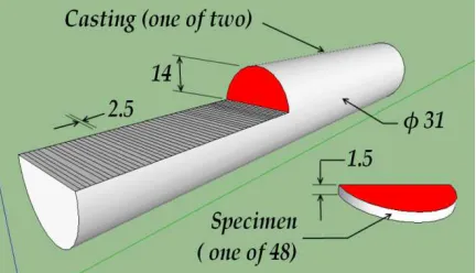
The machining cuts which were performed on the specimens were 48 in number. These were carried out in accordance with the conditions described by the l-16 orthogonal array. Each of these cuts was 14 mm deep, and all these cuts were placed mutually at an axial distance of 2.5 mm. The model is shown in
Figure 1, and the actual cut out pieces have been shown in Figure 2.
[image:2.595.309.525.475.599.2]3834
Fig. 2. The cut out semi-circular disc-shaped
specimens whose surfaces had to be analyzed for their microhardness values and considered in the Taguchi method.
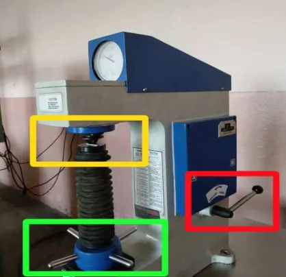
The microhardness values of these tests had been performed on the Rockwell hardness testing machine with diamond tip indenter, as shown in Figure 3.
Fig. 3. Rockwell microhardness testing machine (details). The yellow rectangle indicates the turret on which the specimen was needed to be placed, the green rectangle shows the hand wheel for application of minor load on the specimen, and the red rectangle
shows the lever for the release of major load on the surface of specimen by the indenter.
In order to conduct the microhardness tests of the pieces obtained from the specimens after wire EDM machining, according to tables, the diamond tip indenter for a load of 60 kg was selected. This indenter was mounted on the turret upside down over the test table. After a specific semi-circular disc-shaped specimen was placed with its test surface
towards the top on the test table whose position has been shown by a yellow circle, the hand wheel beneath it was rotated so as to raise it to touch the indenter.
3. RESULTS AND DISCUSSION
3.1.Design of experiments
[image:3.595.70.290.310.448.2]For the sake of accuracy, five readings had been taken on the surface of each specimen at various random places, and their averages had been considered in the study. These readings have been shown in Table 2 below.
Table 2. Microhardness values of specimens
( numbered 1 to 48)
N
o
.
o
f
sp
ec
im
en
M
ic
ro
h
a
rd
n
es
s
a
t
1
st
p
la
ce
(
H
R
A
)
M
ic
ro
h
a
rd
n
es
s
a
t
2
n
d
p
la
ce
(
H
R
A
)
M
ic
ro
h
a
rd
n
es
s
a
t
3
rd
p
la
ce
(
H
R
A
)
M
ic
ro
h
a
rd
n
es
s
a
t
4
th
p
la
ce
(
H
R
A
)
M
ic
ro
h
a
rd
n
es
s
a
t
5
th
p
la
ce
(
H
R
A
)
A
ve
ra
g
e
m
ic
ro
h
a
rd
n
es
s
(H
R
A
)
1 95 67 69 78 67 75.2
2 86 76 84 79 62 77.4
3 82 85 83 86 87 84.6
4 90 75 90 82 82 83.8
5 81 84 75 94 82 83.2
6 86 78 88 86 82 84.0
7 54 69 73 74 67 67.4
8 79 70 82 79 77 77.4
9 76 60 73 83 67 71.8
10 76 78 68 85 76 76.6
11 85 85 90 90 88 87.6
12 86 88 86 87 78 85.0
13 86 86 88 85 88 86.6
14 92 89 95 89 84 89.8
15 80 84 83 86 87 84.0
16 58 80 72 78 78 73.2
17 60 75 62 82 83 72.4
18 70 48 83 30 77 61.6
19 80 91 89 89 87 87.2
20 90 91 92 94 89 91.2
21 90 91 90 90 88 89.8
[image:3.595.75.284.563.765.2]3835
23 86 82 94 95 70 85.4
24 83 87 88 84 80 84.4
25 79 86 92 82 82 84.2
26 92 89 81 81 77 84.0
27 89 84 84 91 89 87.4
28 91 92 90 89 87 89.8
29 88 89 91 92 82 88.4
30 88 87 86 88 84 86.6
31 80 75 70 70 90 77.0
32 94 87 92 87 79 87.8
33 92 87 84 91 64 83.6
34 90 91 90 92 90 90.6
35 88 87 90 87 89 88.2
36 89 88 91 94 85 89.4
37 93 93 89 91 93 91.8
38 93 93 92 90 95 92.6
39 89 89 74 94 82 85.6
40 82 87 92 86 83 86.0
41 91 91 93 94 74 88.6
42 88 94 92 73 89 87.2
43 85 88 89 87 86 87.0
44 89 87 93 92 91 90.4
45 89 91 91 92 91 90.8
46 92 91 90 84 91 89.6
47 92 95 95 96 84 92.4
48 52 87 85 96 85 81.0
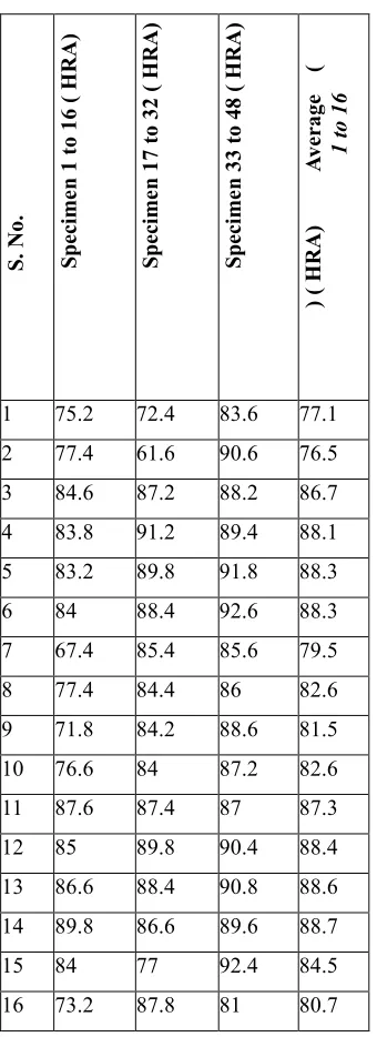
[image:4.595.310.480.93.560.2]The Taguchi l-16 orthogonal array used in this work directs to use 16 experimental trials. For the sake of accuracy, each of these tests had been performed 3 times, because of which, the total number of tests had come out to be 48 (16x3). This was done in accordance with the concept of repetition. These are the 16 settings which have been directed by the l-16 orthogonal array in accordance to which these 48 tests had been performed. Table 3 shows these 16 values which we next used in the orthogonal array.
Table 3. Average micro hardness obtained during machining at each setting of Orthogonal Array (numbered 1 to 16)
S
.
N
o
.
S
p
ec
im
e
n
1
t
o
1
6
(
H
R
A
)
S
p
ec
im
e
n
1
7
t
o
3
2
(
H
R
A
)
S
p
ec
im
e
n
3
3
t
o
4
8
(
H
R
A
)
A
v
er
a
g
e
(
1
t
o
1
6
)
(
H
R
A
)
1 75.2 72.4 83.6 77.1
2 77.4 61.6 90.6 76.5
3 84.6 87.2 88.2 86.7
4 83.8 91.2 89.4 88.1
5 83.2 89.8 91.8 88.3
6 84 88.4 92.6 88.3
7 67.4 85.4 85.6 79.5
8 77.4 84.4 86 82.6
9 71.8 84.2 88.6 81.5
10 76.6 84 87.2 82.6
11 87.6 87.4 87 87.3
12 85 89.8 90.4 88.4
13 86.6 88.4 90.8 88.6
14 89.8 86.6 89.6 88.7
15 84 77 92.4 84.5
16 73.2 87.8 81 80.7
[image:4.595.74.280.98.413.2]As per the standard method of Taguchi analysis of orthogonal arrays, these 16 values had been placed on the right side of the l-16 orthogonal array, as shown in Table 4 below.
Table 4. Orthogonal Array l 16 for microhardness
L
ev
el
4
1
.2
5
A 7
2 V
1
2
0
0
g
2
.5
l
.p
.m
[image:4.595.307.528.651.714.2]3836
L ev el 3 1 .0 0 A 6 8 V 11 0 0 g 2 .0 l .p .m . A ve ra g e m ic ro h a rd n es s (H R A ) L ev el 2 1 0 % S iC 5 0 m m 5 m /m in 0 .7 5 A 6 4 V 1 0 0 0 g 1 .5 l .p .m . L ev el 1 5 % S iC 4 0 m m 3 m /m in 0 .5 0 A 6 0 V 9 0 0 g 1 .0 l .p .m . F a ct o rs W o rk -p ie ceUpp
er n o zz le h ei g h t W ir e fe ed r a te C u rr en t G a p v o lt a g e T en si o n U p p er n o zz le f lo w r a te E x p . tr ia l n o . F a ct o r A F a ct o r B F a ct o r C F a ct o r D F a ct o r E F a ct o r F F a ct o r G
1 1 1 1 1 1 1 1 77.1 2 1 2 2 1 2 2 2 76.5 3 2 1 2 1 3 3 3 86.7 4 2 2 1 1 4 4 4 88.1 5 2 2 1 2 1 2 1 88.3 6 2 1 2 2 2 1 2 88.3 7 1 2 2 2 3 4 4 79.5 8 1 1 1 2 4 3 3 82.6 9 1 2 2 3 1 3 4 81.5 10 1 1 1 3 2 4 3 82.6 11 2 2 1 3 3 1 2 87.3 12 2 1 2 3 4 2 1 88.4 13 2 1 2 4 1 4 2 88.6 14 2 2 1 4 2 3 1 88.7 15 1 1 1 4 3 2 4 84.5 16 1 2 2 4 4 1 3 80.7
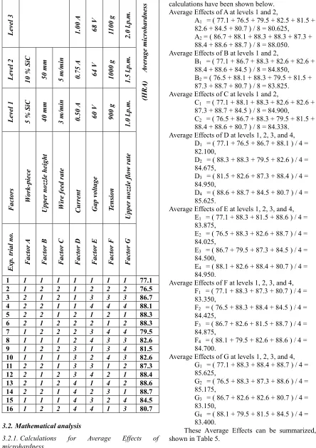
3.2.Mathematical analysis
3.2.1.Calculations for Average Effects of microhardness
Based on Table 4 given above, next, the Average Effects of microhardness were calculated. The
calculations have been shown below. Average Effects of A at levels 1 and 2,
A1 = ( 77.1 + 76.5 + 79.5 + 82.5 + 81.5 +
82.6 + 84.5 + 80.7 ) / 8 = 80.625,
A2 = ( 86.7 + 88.1 + 88.3 + 88.3 + 87.3 +
88.4 + 88.6 + 88.7 ) / 8 = 88.050. Average Effects of B at levels 1 and 2,
B1 = ( 77.1 + 86.7 + 88.3 + 82.6 + 82.6 +
88.4 + 88.6 + 84.5 ) / 8 = 84.850,
B2 = ( 76.5 + 88.1 + 88.3 + 79.5 + 81.5 +
87.3 + 88.7 + 80.7 ) / 8 = 83.825. Average Effects of C at levels 1 and 2,
C1 = ( 77.1 + 88.1 + 88.3 + 82.6 + 82.6 +
87.3 + 88.7 + 84.5 ) / 8 = 84.900,
C2 = ( 76.5 + 86.7 + 88.3 + 79.5 + 81.5 +
88.4 + 88.6 + 80.7 ) / 8 = 84.338. Average Effects of D at levels 1, 2, 3, and 4,
D1 = ( 77.1 + 76.5 + 86.7 + 88.1 ) / 4 =
82.100,
D2 = ( 88.3 + 88.3 + 79.5 + 82.6 ) / 4 =
84.675,
D3 = ( 81.5 + 82.6 + 87.3 + 88.4 ) / 4 =
84.950,
D4 = ( 88.6 + 88.7 + 84.5 + 80.7 ) / 4 =
85.625.
Average Effects of E at levels 1, 2, 3, and 4,
E1 = ( 77.1 + 88.3 + 81.5 + 88.6 ) / 4 =
83.875,
E2 = ( 76.5 + 88.3 + 82.6 + 88.7 ) / 4 =
84.025,
E3 = ( 86.7 + 79.5 + 87.3 + 84.5 ) / 4 =
84.500,
E4 = ( 88.1 + 82.6 + 88.4 + 80.7 ) / 4 =
84.950.
Average Effects of F at levels 1, 2, 3, and 4,
F1 = ( 77.1 + 88.3 + 87.3 + 80.7 ) / 4 =
83.350,
F2 = ( 76.5 + 88.3 + 88.4 + 84.5 ) / 4 =
84.425,
F3 = ( 86.7 + 82.6 + 81.5 + 88.7 ) / 4 =
84.875,
F4 = ( 88.1 + 79.5 + 82.6 + 88.6 ) / 4 =
84.700.
Average Effects of G at levels 1, 2, 3, and 4,
G1 = ( 77.1 + 88.3 + 88.4 + 88.7 ) / 4 =
85.625,
G2 = ( 76.5 + 88.3 + 87.3 + 88.6 ) / 4 =
85.175,
G3 = ( 86.7 + 82.6 + 82.6 + 80.7 ) / 4 =
83.150,
G4 = ( 88.1 + 79.5 + 81.5 + 84.5 ) / 4 =
83.400.
[image:5.595.69.513.101.729.2]These Average Effects can be summarized, as shown in Table 5.
3837
F a ct o r F a ct o r n a m e L ev el 1 , L 1 L ev el 2 , L 2 L ev el 3 , L 3 L ev el 4 , L 4A Work-piece
80.625 88.050 - -
B Upper nozzle height
84.850 83.825 - -
C Wire feed rate
84.900 84.338 - -
D Current 82.100 84.675 84.950 85.625
E Gap voltage
83.875 84.025 84.500 84.950
F Tension 83.350 84.425 84.875 84.700
G Upper nozzle flow rate
85.625 85.175 83.150 83.400
3.3.2.Calculations for sum of squares of factors and their percentage contribution
Based on Table 5 given above, next, the sum of squares of each factor is calculated. The relation used here is shown in Eq. (1),
SS =
(1)
Here, xm is the Mean of Levels which have been
calculated in Table 6, n is the degrees of freedom, taken as one for all two-level factors and three for all four-level factors, and other terms have their usual notations.
[image:6.595.67.302.100.348.2]Furthermore, these sum of squares have been used to calculate the percent contribution of various factors for microhardness. This has been shown in Table 6 to Table 9 below.
Table 6. Means of Levels (to calculate Percent Contribution for microhardness)
F
a
ct
o
r L
ev el 1 , L 1 L ev el 2 , L 2 L ev el 3 , L 3 L ev el 4 , L 4 M ea n o f L ev el s (x m )
A 80.625 88.050 - - 84.34
B 84.850 83.825 - - 84.338
C 84.900 83.775 - - 84.338
D 82.100 84.675 84.950 85.625 84.338
E 83.875 84.025 84.500 84.950 84.338
F 83.350 84.425 84.875 84.700 84.338
G 85.625 85.175 83.150 83.400 84.338
Table 7. Calculations of Percent Contribution for microhardness F a ct o r L 1 x m L 2 x m L 3 x m L 4 x m
A -3.713 3.712 - -
B 0.512 -0.513 - -
C 0.562 -0.563 - -
D -2.238 0.337 0.612 1.287
E -0.463 -0.313 0.162 0.612
F -0.988 0.087 0.537 0.362
G 1.287 0.837 -1.188 -0.938
Table 8. Sum of squares (to calculate Percent Contribution for microhardness)
F a ct o r (L 1 -x m ) 2 (L 2 -x m ) 2 (L 3 -x m ) 2 (L 4 -x m ) 2 Σ
A 13.78
6
13.77
9
- - 27.5
65
B 0.262 0.263 - - 0.52
5
C 0.316 0.317 - - 0.63
3
D 5.009 0.114 0.375 1.656 7.15
3
E 0.214 0.098 0.026 0.375 0.71
3
F 0.976 0.008 0.288 0.131 1.40
3
G 1.656 0.701 1.411 0.880 4.64
∑
x−xm
2
[image:6.595.197.492.490.772.2]3838
8Table 9. Percent Contribution for microhardness
F
a
ct
o
r
Σ
D
.F
.
(n
)
S
u
m
o
f
sq
u
a
re
s
A 27.565 1 27.565
B 0.525 1 0.525
C 0.633 1 0.633
D 7.153 3 2.384
E 0.713 3 0.238
F 1.403 3 0.468
G 4.648 3 1.549
[image:7.595.74.209.177.414.2]The percent contribution of various factors has been shown graphically in Figure 4.
Fig. 4. A bar chart showing the percent contribution of various factors in the wire EDM machining of Al-SiC 6061 alloy.
3.3.Determination of factor levels for achieving
maximum microhardness values
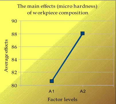
As per the Taguchi technique, the main effects of microhardness need to be plotted graphically for each factor, one by one. This is done by plotting the Average Effects of that factor on two-dimensional graph, as shown in Figure 5.
3.3.1.
In the context of the SiC percentage of both the specimens, the plots of the main effects have been
shown below.
The Average Effects, depicted in Table 5 have been plotted along the y-axis and the levels of factors have been plotted along the x-axis in Figure 5.
Fig. 5. Graphical representation of the main effects of factor A (both specimens' SiC percentage). Y-axis has Average Effects in units of HRA and X-axis has 5% SiC composition specimen as A1 and 10% SiC composition as A2.
The microhardness needs to be maximized. Hence, on the visual examination of Figure 5 above, we see that the factor level that shall result in a higher value of microhardness is A2.
3.3.2.
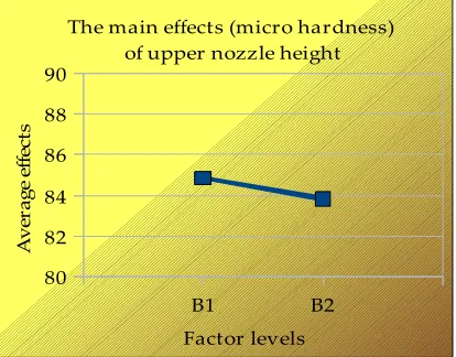
In the context of the upper nozzle height of the wire EDM machine, the plots of the main effects have been shown below.
Gap voltage Tension Upper nozzle height Wire f eed rate Upper nozzle f low rate Current Work-piece
0 10 20 30 40 50 60 70 80 90
A1 A2
80 82 84 86 88 90
The main effects (micro hardness) of w orkpiece composition
Factor levels
A
v
er
a
g
e
ef
fe
ct
[image:7.595.310.512.529.710.2]3839
The Average Effects, depicted in Table 5 have beenplotted along the y-axis and the levels of factors been plotted along the x-axis in Figure 6.
Fig. 6. Graphical representation of the main effects of factor B (upper nozzle height). Y-axis has Average Effects in units of HRA and X-axis has 40 mm as B1 and 50 mm as B2.
We see that the factor level that shall result in a higher value of microhardness is B1.
3.3.3.
In the context of the wire feed rate, the plots of the main effects have been shown below.
The Average Effects, depicted in Table 5 have been
[image:8.595.74.281.259.421.2]plotted and the levels of factors have been plotted along the x-axis in Figure 7.
Fig. 7. Graphical representation of the main effects of factor C (wire feed rate). Y-axis has Average Effects in units of HRA and X-axis has wire feed rate as level C1 and level C2 in units of m/min.
The microhardness needs to be maximized. Hence, on the visual examination of Figure 7 above, we see that the factor level that shall result in a higher value of microhardness is C1.
3.3.4.
In the context of the (machining) current used in the Wire EDM machine, the plots of the main effects have been shown below.
The Average Effects, depicted in Table 5 have been plotted along the y-axis and the levels of factors have been plotted along the x-axis in Figure 8.
Fig. 8. Graphical representation of the main effects of factor D (machining current). Y-axis has Average Effects in units of HRA and X-axis has machining current as a factor at levels D1, D2, D3, and D4 in units of amperes.
The microhardness needs to be maximized. Hence, on the visual examination of Figure 8 above, we see that the factor level that shall result in a higher value of microhardness is D3.
3.3.5.
In the context of the gap voltage between the electrode wire of the Wire EDM machine and the workpiece to
be machined, the plots of the main effects have been shown below.
The Average Effects, depicted in Table 5 have been plotted along the y-axis and the levels of factors have been plotted along the x-axis in Figure 9.
B1 B2
80 82 84 86 88 90
The main effects (micro hardness) of upper nozzle height
Factor levels
A
v
er
a
g
e
ef
fe
ct
s
C1 C2
80 81 82 83 84 85 86 87 88 89 90
The main effects (micro hardness) of wire feed rate
Factor levels
A
v
er
a
g
e
ef
fe
ct
[image:8.595.72.284.563.759.2]3840
Fig. 9. Graphical representation of the main effects offactor E (gap voltage ). Y-axis has Average Effects in units of HRA and X-axis has gap voltage as a factor at levels E1, E2, E3, and E4 in units of volts.
The microhardness needs to be maximized. Hence, we see that the factor level that shall result in a higher value of microhardness is E4.
3.3.6.
[image:9.595.72.294.109.304.2]In context of the wire tension, the Average Effects have been plotted along the y-axis and the levels of factors along the x-axis in Figure 10.
Fig. 10. Graphical representation of the main effects of factor F (wire tension ). Y-axis has Average Effects in units of HRA and X-axis has (wire) tension as a factor at levels F1, F2, F3, and F4 in units of grams.
The microhardness needs to be maximized. Hence, on the visual examination of Figure 10 above, we see that
the factor level that shall result in a higher value of microhardness is F3.
3.3.7.
In the context of the upper nozzle flow rate, the plots of the main effects have been shown below.
The Average Effects, depicted in Table 5 have been plotted along the y-axis and the levels of factors have been plotted along the x-axis in Figure 11.
Fig. 11. Graphical representation of the main effects of factor G (upper nozzle flow rate). Y-axis has Average Effects in units of HRA and X-axis has upper nozzle flow rate as a factor at levels G1, G2, G3, and G4 in units of l.p.m.
The microhardness needs to be maximized. Hence, on the visual examination of Figure 11 above, we see that the factor level that shall result in a higher value of microhardness is G1.
From the visual examination of figures above, we see that the levels of various factors that shall result in a high value of microhardness correspond to A2 B1C1 D3 E4 F3 G1.
[image:9.595.306.529.209.403.2]3841
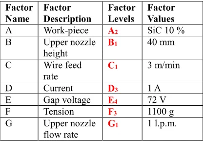
Table 10. Levels of factors for maximization ofmicrohardness
Factor Name
Factor Description
Factor Levels
Factor Values
A Work-piece A2 SiC 10 %
B Upper nozzle
height
B1 40 mm
C Wire feed
rate
C1 3 m/min
D Current D3 1 A
E Gap voltage E4 72 V
F Tension F3 1100 g
G Upper nozzle
flow rate
G1 1 l.p.m.
It is deemed that the above-mentioned levels of the given factors were to result in a higher value of microhardness.
3.4.Projection of optimal performance (microhardness)
According to the usual notations, here, Number of observations, N = 16 Total of all observations, T
According to the usual notations, here, Total number of observations, N = 16 Sum total of all observations, T
= 77.1 + 76.5 + 86.7 + 88.1 + 88.3 + 88.3 + 79.5 + 82.6 + 81.5 + 82.6 + 87.3 + 88.4 + 88.6 + 88.7 + 84.5 + 80.7
= 1349.4. Optimal performance,
Yoptimal = T/N + ( A2 - T/N ) + ( B1 – T/N ) +
( C1 – T/N ) + ( D3 - T/N ) + ( E4 - T/N) + ( F3
– T/N ) + ( G1 – T/N ),
= 84.338 + (88.050- 84.338) + (84.850-
84.338) + (84.900- 84.338) + (84.950-
84.338) +
(84.950- 84.338) + (84.875- 84.338) +
(85.625 - 84.338),
= 84.338 + (3.712) + (0.512) + (0.562) +
( 0.612) + (0.612) + (0.537) + (1.287) ,
= 92.172 HRA. 4. CONFIRMATION TESTS
It is recommended that the projected optimal
performance should be checked by running
confirmatory tests. After the aforesaid calculations were made, confirmatory experiments were carried out as per the parameter settings of Table 10.
A total of three tests were performed, and hence, three specimens were prepared. All these specimens were prepared from the SiC 10 % composition casting which corresponds to A2. In order to prepare these specimens, the SiC 10 % composition casting was mounted on the Wire EDM machine. The various parameters were set according to the Table 10, after which, the machining cuts were made on the casting. This resulted in three specimens which had been cut on the parameter settings recommended for obtaining maximum microhardness value. Similar to the earlier cut specimens during the test, the microhardness values were measured on all these three specimens at five random points on their surfaces on the same microhardness testing machine, and the average of these five points was taken. Then the average microhardness values of these three specimens were taken. The readings have been shown in Table 11 below.
Table 11. Confirmation tests for microhardness
S
p
ec
im
e
n
n
u
m
b
er
M
ic
ro
-h
a
rd
n
e
ss
(H
R
A
)
A
v
er
a
g
e
(H
R
A
)
O
v
er
a
ll
a
v
er
a
g
e
(H
R
A
)
1
st
re
a
d
in
g
2
n
d
re
a
d
in
g
3
rd
re
a
d
in
g
4
th
re
a
d
in
g
5
th
re
a
d
in
g
C 1
90 89 91 90 90 90.000 91.13
C 2
90 91 93 90 90 90.800
C 3
92 91 93 94 93 92.600
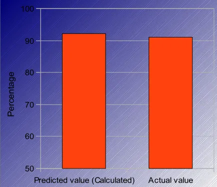
These results have been shown graphically in Figure 12 on being compared with their accuracy of predicted values.
[image:10.595.307.528.336.636.2]3842
Fig. 12. Comparison of predicted and actual values ofmicrohardness obtained after the confirmation tests.
5. CONCLUSIONS AND FUTURE SCOPE
It has been found out in this study that during the machining of Al-SiC MMC material carried out on a Wire EDM machine, the factor which most significantly affects the microhardness of the
specimens is the work-piece composition, that is, the percentage of reinforcement phase, SiC particles in this case. Clearly, a 10% SiC composition aluminum MMC gives greater hardness values than 5% SiC composition one. Similar had been the results by Karthick et al. in an earlier study regarding magnesium based MMCs [14]. After that, the various factors which affect the microhardness values of surface machined out by Wire EDM machine in the decreasing order of significance are (machining) current, upper nozzle flow rate, wire feed rate, upper nozzle height, wire tension, and gap voltage, respectively.
It was seen that with the design of experiments being done in accordance with the Taguchi technique, we were able to achieve quite high values of surface microhardness. Wire EDM is a non-conventional machining process employed for the machining of difficult to machine materials which are too hard to be machined by conventional processes.
Hardness is an important property which should be preserved and enhanced during a machining process. This paper puts forward an experimental technique by which an optimal combination of parameters may be determined which results in higher values of surface microhardness. This is liable to result in higher operating lives of products obtained after machining, for example, the extrusion dies which are obtained by
the operation of taper cutting carried on wire EDM machines. It also lays down a possibility that the microhardness values can be planned well in advance of the surfaces which shall be obtained during wire EDM machining. For example, in order to obtain less brittle surface in some specific requirement, lower values of microhardness could also be achieved by this method.
REFERENCES
[1] H. Liu. “7M” Advantages of Abrasive Waterjet
for Machining Advanced Materials”. J. Manuf. Mater. Process, volume 1, page 11, 2017.
[2] P. Vundavilli and J. Kumar, C. Priyatham.
“Parameter optimization of wire electric discharge machining process using GA and PSO”. In IEEE-International Conference On Advances In
Engineering, Science And Management
(ICAESM -2012), Nagapattinam, Tamil Nadu, pages 180-185, 2012.
[3] Y. Ahmed, H. Youssef, and H. Hofy. “Prediction
and Optimization of Drilling Parameters in Drilling of AISI 304 and AISI 2205 Steels with PVD Monolayer and Multilayer Coated Drills”. J. Manuf. Mater. Process., volume 2(1), page 16, 2018.
[4] “Advanced Materials by design”. Washington DC,
US Government Printing Office, chapter 1, page 9, 1988.
[5] N. Muthukrishnan and J. Davim. “Optimization of
Machining Parameters of Al/SiC-MMC with ANOVA and ANN Analysis”. Journal of Materials Processing Technology, volume 209 (1), pages 225–232, 2009.
[6] K. Prasad and K. Jayadevan. “Simulation of
Stirring in Stir Casting”. Procedia Technol, volume 24, pages 356-363, 2016.
[7] P. Ross. “Taguchi Techniques for Quality
Engineering: Loss Function, Orthogonal
Experiments, Parameter and Tolerance Design”. McGraw-Hill. ISBN 978-0442237295, 1996.
[8] R. Singh, R. Singh, and J. Dureja, I. Farina, F.
Fabbrocino. “Investigations for Dimensional Accuracy of Al Alloy/Al-MMC Developed by Combining Stir Casting and ABS Replica Based
Investment Casting”. Composites Part B:
Engineering, volume 115, pages 203–208, 2017.
[9] A. Satpathy, S. Tripathy, N. Senapati, and M.
Brahma. “Optimization of EDM Process
Parameters for Al-SiC-20% SiC Reinforced Metal Matrix Composite with Multi Response Using TOPSIS”. Materials Today: Proceedings, volume 4 (2), pages 3043–3052, 2017.
[10] K. Hamim, S. Akbari, S. Fakhrhoseini, H.
Khayyam, A. Pakseresht, E. Ghasali, M. Zabet, and K. Munir. Ji. “Carbon Fiber Reinforced Metal Predicted value (Calculated) Actual value
50 60 70 80 90 100
P
e
rc
e
n
ta
g
3843
Matrix Composites: Fabrication Processes andProperties”. Composites Part A: Applied Science and Manufacturing, volume 92, pages 70–96, 2017.
[11] A. Gore and N. Patil. “Wire Electro Discharge
Machining of Metal Matrix Composites: A Review”. Procedia Manufacturing, volume 20, pages 41–52, 2018.
[12] R. Garg and H. Singh. “Optimisation of Process
Parameters for Gap Current in Wire Electrical Discharge Machining”. International Journal of Manufacturing Technology and Management, volume 25, page 161, 2012.
[13] A. Roy, and K. Kumar. “Effect and Optimization
of Various Machine Process Parameters on the Surface Roughnes in EDM for an EN19 Material using Response Surface Methodology”. Procedia Mater. Sci., volume 5, pages 1702-1709, 2014.
[14] J. Mathai, J. Tony, and S. Marikkannan.
“Processing, Microstructure and Mechanical