Rapid Binary Gage Function to Extract
a Pulsed Signal Buried in Noise
Colin Ratcliffe
Mechanical Engineering Department, United States Naval Academy, Annapolis, MD 21402, USA Email:ratcliff@usna.edu
William J. Bagaria
Aerospace Engineering Department, United States Naval Academy, Annapolis, MD 21402, USA Email:[email protected]
Sonia M. F. Garcia
Mathematics Department, United States Naval Academy, Annapolis, MD 21402, USA Email:[email protected]
Richard P. Fahey
Aerospace Engineering Department, United States Naval Academy, Annapolis, MD 21402, USA Email:[email protected]
Received 1 August 2003; Revised 14 January 2004; Recommended for Publication by Sang Uk Lee
The type of signal studied in this paper is a periodic pulse, with the pulse length short compared to the period, and the signal is buried in noise. If standard techniques such as the fast Fourier transform are used to study the signal, the data record needs to be very long. Additionally, there would be a very large number of calculations. The rapid binary gage function was developed to quickly determine the period of the signal, and the start time of the first pulse in the data. Once these two parameters are determined, the pulsed signal can be recovered using a standard data folding and adding technique.
Keywords and phrases:rapid binary gage function, signal, pulsed signal, noise.
1. INTRODUCTION
The motivation for this research was the need to extract pulsed signals that were buried in noise (signal-to-noise ra-tio less than one). The signals of interest have a “short” pulse duration compared to the period of the signal, and they are “weak” compared to the background noise. Another consid-eration when analyzing these signals was that the length of the recorded signal be as short as possible.
Classic techniques for recovering information about noisy signals are usually based on the Fourier transform [1], the periodogram [2], or simply folding and adding the data. When dealing with digitized data, certain precautions must be taken when the data are analyzed. The signal must be dig-itized based on the Nyquist sampling rate, which in turn is based on the highest desired frequency component of the signal. This is to avoid the appearance of false aliases in the Fourier transform. Generally, to avoid this, the analog signal is first lowpass filtered before being digitized [3].
Difficulties arise when recording and analyzing signals which have a pulse duration that is short when compared to the pulse period. Such a signal contains frequency com-ponents that are very high compared to the fundamental fre-quency of the signal. For pulsed signals, the digitizing rate must be sufficiently high so that the pulse is well defined. This means that the sampling rate is dictated by the pulse duration, and not the period of the signal. The use of filters to precondition this type of signal when it is buried in noise might in fact result in the pulse being completely filtered out of the data. Additionally, when the signal is buried in noise, the classic techniques, when applied to high frequency sig-nals, require long data records. This in turn, necessitates very long times to acquire and analyze the data.
Pulse period
3.5 4 4.5 5 5.5 6 6.5 7 7.5 Time (s)
Figure1: Signal from pulsar PSR B0329 + 54 captured by a 12 m antenna.
pulse rate measured from a number of pulsars. These shifts can be used to identify the direction of travel, and ultimately the position of the Earth or any other interplanetary space vehicle. One candidate pulsar is PSR B0329 + 54, which has a period of 0.715 seconds and a pulse width of approximately 8.7 milliseconds. An example of data captured from this pul-sar using a 12-meter parabolic antenna is shown inFigure 1. Data capture for this data set started on 3/3/98 at 21:20:46 GMT, and the sample rate was 1000 samples per second. The time record shown in the figure should include several pulses, but these cannot be seen because the pulsed signal is com-pletely buried in noise.
The spectral resolution of the pulse rate required for sat-isfactory interplanetary navigation using this pulsar is about 3µHz. If classical FFT analysis were selected for this problem, the Nyquist sampling rate and FFT theory control the length of an individual time record to 1/(required spectral resolu-tion). For this pulsar the required record length is 330 000 seconds, or nearly 4 days. Clearly, a single data record would be insufficient to extract the pulse from the noise. It is esti-mated that at least 100 averages would be required for satis-factory extraction. Thus, the total data capture would take at least 33×106seconds, or 385 days. It is impossible to main-tain the alignment of a single earthbound dish for this length of time since the rotation of the Earth typically limits data acquisition to less than half a day at a time. This aside, the process would eventually produce an average position of the Earth during data acquisition and the ability to locate the Earth within its orbit is lost. Thus, FFT-based methods can-not be used for this navigational application because the fix time of 385 days is comparable to the journey time!
These and other considerations led to the development of a non-FFT-based technique to recover a pulsed signal buried in noise. The procedure developed in this paper can deter-mine the pulse period using data acquired in only a few min-utes, thus permitting close to real-time analysis.
The paper is divided into two parts. First, a method is presented that allows the rapid determination of the period of the signal, and the start time of the first pulse in the data. Second, the time-averaged wave form shape of the pulsed sig-nal is recovered from the noisy data.
2. NOISY DATA
Consider a data signalD(t) which is the sum of a periodic pulsed signalF(t) and noiseN(t). Example signals are shown in Figures2aand2b.
Notice that the vertical scales of Figures2aand2bare dif-ferent. The pulsed signal,F(t), has a period ofTF. The pulse width,TF/KF, is given in terms of the period, and a constant KF, withKFbeing called the pulse width parameter. It is
ex-pected that the beginning of the first pulse, in the recorded data, does not start att=0. The timetSF shifts the pulse in time to account for this. The signalF(t) shown inFigure 2a
can be generated using the following equations:
F(t)
In this equation,CN is the cycle number,Cis the maxi-mum number of cycles, andAFis the maximum amplitude of F(t). The pulse width parameter takes on the valuesKF≥1. IfKF=1, then the pulse width is equal to the period. It is to be noted thatKFprobably will not be an integer.
The mean value of a pulsed signal is not necessarily equal to zero. The mean value of the exampleF(t) is ¯f =2AF/πKF, and is nonzero. Because ¯f may not be equal to zero, we do not average out the mean value ofD(t) before analyzing the signal as is usually done [4]. This also means that a nonzero mean value of the noise would not be removed.
Mathematically, define
F(t)= f(t) + ¯f,
N(t)=ν(t) + ¯ν, (2)
where f(t) is the zero-mean time-varying part of the pulsed signalF(t), and ¯f is the mean value. The zero-mean time-varying part of the noise,N(t), isν(t), and ¯νis the nonzero mean value. Using the above definitions, the observed data signal is given by
D(t)=F(t) +N(t)= f(t) + ¯f +ν(t) + ¯ν. (3)
For storage and analysis purposes, the data signal is digi-tized. The inverse of the sampling rate ish, with units of sec-onds/sample. The total number of data points isn =tR/h. Here,nis an integer, andtR is the total time of the record length.
3. DISCRETE CROSS-CORRELATION FUNCTION
F(t) AF
¯ f
0
tSFtSF+TF KF TF
tR t
(a)
D(t)
¯ ν
0 t
(b)
Figure2: (a) Pulsed signalF(t) versus timet. (b) Data signalD(t)=F(t) +N(t) versus timet.
biased discrete cross-correlation function is then given by
ˆ
Rxy(rh)= 1n n−r
i=1
xiyi+r, r=0, 1, 2,. . .,m≤n−1. (4)
In this equation,ris the lag number. Thenrhis the lag time between yandx. The lag timerhis the digital equiv-alent of the continuous lag time τ. Notice, asr approaches n−1 there are fewer and fewer terms which are added to-gether. This results in a loss of accuracy for high lag times [1]. Two important properties of the cross-correlation func-tion, [1,5], are
Rˆxy(rh)2
≤Rˆx(0) ˆRy(0),
Rˆxy(rh)≤ 1
2
ˆ
Rx(0) + ˆRy(0) .
(5)
In these relationships, ˆRxand ˆRyare the autocorrelation functions of x and y, respectively. Another property arises when bothxand yare periodic, with thesameperiod. For this special case, the cross-correlation function is also pe-riodic, with the same period as x and y [1]. A significant disadvantage of using the autocorrelation function is the large number of calculations that need to be performed. It requires (n2+n)/2 multiplications, and (n2+n)/2 additions for the direct method, although FFT methods can reduce the number of multiplications tonlogn.
4. MODIFIED DISCRETE CROSS-CORRELATION FUNCTION
For the purposes of this research, the discrete cross-correlation function, (4), was modified. Thexiterm was re-placed with the data,Di, withi=1, 2,. . .,n. Theyiterm was replaced with a pulsed periodic reference function called the
binary gage. It is defined as follows:
G(t,T,K)=
0 outside the pulse,
1 during the pulse. (6)
The pulses occur during the times
τ+CN−1T≤t≤τ+CN−1T+ T
K (7) with
CN =1, 2,. . .,C. (8)
Here,Tis the period, andKis the pulse width parameter of the binary gage. The binary gage is illustrated inFigure 3. Notice that the binary gage is not a Walsh or related function [1,6] which are square waves with values of±1. The binary gage only takes on the values 0 and 1 and has variable period Tand pulse width parameterK.
The binary gage is digitized with the samehvalue as was used for the data. However, to increase accuracy, it is twice as long as the length of the data set. The digitized binary gage is Gj, withj=1, 2,. . .,n,. . ., 2n. Since the binary gage is twice as long asDi, the summation upper limit in (4) becomesn. Using these substitutions, and multiplying through byn, (4) becomes
nRˆDG(rh)=n
i=1
DiGi+r, r=0, 1,. . .,n−1. (9)
The effect of the noise on (9) can be illustrated by substi-tutingDi=Fi+νi+ ¯ν. This gives
nRˆDG(rh)
= n
i=1
FiGi+r+ n
i=1
νiGi+r+ ¯ν n
i=1
Gi+r, r=0, 1,. . .,n−1.
G(t,T,K)
The first term on the right is the cross-correlation of the pulsed signal with the binary gage. When the period of the binary gage is the same as the period of the pulsed signal, the cross-correlation will have the same period. The second term on the right is the cross-correlation of the noise with the bi-nary gage. The pieces of equipment used to receive, digitize, and store the data signal have finite band widths. Thus,νiis band-limited white noise (pink noise). This means that the second term on the right will not exactly sum to zero. The third term is a result of the mean value of the noise not being zero. In this equation, it is implied that the noise is station-ary and ergodic. Strictly speaking, the noise only has to have these features during the time of the data record.
5. RAPID BINARY GAGE FUNCTION
The purpose of therapid binary gage function(RBGF) is to rapidly determine the period,TF, of the signal, and the start time,tSF, of the first pulse. The properties of the binary gage are used to reduce the number of computations. During the pulse, the binary gage has a value of one. Thus, there is no need to perform these multiplications. Outside the pulse, the binary gage has a value of zero. Thus, there is no need to per-form these multiplications or adds. Equation (9) can now be written as only during the pulse of the binary gage. Otherwise, incre-mentito the next value.
There are significant computational savings for (11) compared to (4) and (9). First, there are no multiplications. Second, the RBGF will be periodic, with the period ofF(t), whenG(t) has the period ofF(t). This means that the
max-imum lag numberr only needs to equalT/h. This results in a further savings of computations. The resulting number of adds isnT/Kh.
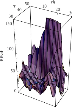
The use of the RBGF requires an estimate ofK, the pulse width parameter of the binary gage. It also requires estimates of the low,TL, and high,TH, values of the period of the binary gage. The behavior of the RBGF is seen when a surface plot is generated. For eachK, plot the values of RBGF versusTand rh. WhenTLandTHbracketTF, there will be a peak in the plot whenT=TFandrh=tSF. An algorithm for calculating the RBGF is given inAlgorithm 1.
Example RBGF plots are shown in Figures4,5,6, and7. These plots use theF(t) equation that is shown inFigure 2a. For all of the plots the parameters ofF(t) wereAF=7,TF=
40 seconds,KF =4,tR =393 seconds; and the parameters of the binary gage were 30 ≤T ≤50 seconds, 0≤rh≤30 seconds. Notice that in all four plots, the vertical axis scale is shortened compared to the other two axes. The purpose of this was to clarify the plots.
ForFigure 4, the first pulse of the signal started attSF=0 seconds, andK=KF=4.The maximum value of the RBGF
is atT=40 seconds, andrh=0 seconds, which correspond to the parameters ofF(t). The peak value of the RBGF is over 300, which is about 3 times the values of the lower regions of the plot. Thus, TK andtSF can easily be found from the location of the peak value of the RBGF using a simple peak finding program.
ForFigure 5, the first pulse of the signal started attSF = 20 seconds, andK = KF = 4. The maximum value of the RBGF is at T = 40 seconds, andrh = 20 seconds, which correspond to the parameters ofF(t).
Since the binary gage pulse width parameter,K, is esti-mated, it may turn out that it is higher or lower than the sig-nal pulse width parameter,KF. The effects of this are shown in the next two figures.
ForFigure 6,K=2 which is one half the value ofKF=4. This means that the binary gage pulse is twice that of the signal pulse. The first pulse of the signal started attSF =20 seconds. A ridge now appears in the contour plot. The ridge ends atT =40 seconds, andrh=20 seconds, which corre-spond to the parameters ofF(t). Notice that the maximum value is still the same as Figures4and5. This agrees with the theory.
D(j): read in the magnitudes of the data, put them into the arrayD(j),
tR=numeric value of the length of the data record (s),
h=numeric value of the inverse of the signal digitization rate(s/sample),
TL=numeric value of the lowest period of the binary gage (s),
TH=numeric value of the highest period of the binary gage (s),
K=numeric value of the binary gage pulse-duration-parameter,
C=int(tR/TH), minimum number of whole cycles in the data record. int(· · ·)=integer,
rmax=int(TL/h), maximum value of the lag numberr, forT=TLtoTHsteph, set the period of the binary gage,
forr=0 tormax, set the value of the lag number, SUM=0, SUM=temporary variable for summing,
forCN=1 toC,CN=the cycle number,
jL=int((r∗h+ (CN−1)∗T)/h), 1st data point during binary gage pulse,
jH=int((r∗h+ (CN−1)∗T+ (T/K))/h), last data point during binary gage pulse, forj=jLtojH, sum the data points during binary gage pulses,
SUM=D(j) + SUM nextj
nextCN
rh(r)=r∗h,rh=time lag of binary gage,
RBGF(rh,T)=SUM, value of the rapid binary gage function, nextr
nextT
Algorithm1: Rapid binary gage function algorithm.
10 20
30 rh 50
40 30
T
300
200
100
0
RBGF
Figure4: RBGF plot.TF =40 seconds,tSF =0 second, andK =
KF=4.
6. NUMERICAL EXAMPLE
The procedure is demonstrated on a numerically generated signal using parameters comparable to pulsar PSR B0329 + 54.Figure 8shows part of the 60-second long signal that in-cludes an 8.7-millisecond long half-sine pulse being repeated every 0.7415 seconds, with random noise added. The signal has a pulse width parameterKF=85.2. Notice that the pulse width is very small compared with the period of the signal.
10 20
30 rh 50
40 30
T
300
200
100
0
RBGF
Figure5: RBGF plot.TF=40 seconds,tSF=20 seconds, andK=
KF=4.
For the reduced data set shown in the figure, there are pulses starting at times of 0.12 seconds and at 0.861 seconds. The data were digitized at a sampling rate of 1000 samples per second. Clearly a simple visual inspection cannot identify the pulses.
10 20
30 rh 50
40 30
T
300
200
100
0
RBGF
Figure6: RBGF plot.TF =40 seconds,tSF =20 seconds,K =2,
KF=4.
10 20
30 rh 50
40 30
T
150
100
50
0
RBGF
Figure7: RBGF plot.TF =40 seconds,tSF =20 seconds,K =8,
KF=4.
For comparison with earlier work in this paper,Figure 10
shows the same results, but with the area of attention fo-cused around the peak ofFigure 9. The noise in the signal has caused the peak to lose some of the straightforward form seen in the earlier figures. However, the maximum peak is correctly located at rh = 0.7415 seconds and T = 0.12 seconds. Thus the RBGF has correctly located the narrow, pulsed signal hidden in significant noise as was shown in
Figure 8.
7. RECOVERED AVERAGE WAVE FORM
The signal-to-noise ratio of periodic signals can be increased by summing successive periods of the signal [1]. This is not a correlation process, but an averaging one. In order for the noise to average out, the statistical properties of the noise need to be independent of time during the time of the data record. That is, the noise process must be stationary and er-godic [7].
Pulse
0 0.1 0.2 0.3 0.4 0.5 0.6 0.7 0.8 0.9 1 Time (s)
Figure8: Portion of simulated pulsar data.
T 0.7
0.6 0.5
0.4 0.3
0.2 0.1
0
rh 0.73
0.735 0.74
0.745 0.75
Figure9: Results of applying the rapid binary gage function to the simulated pulsar data.
T 0.15
0.14 0.13
0.12 0.11
0.1 0.09
0.08 0.74050.741 rh 0.7415
0.742 0.7425
Figure10: Rapid binary gage function results featuring the region near the peak inFigure 9.
D(j): read in the magnitudes of the data, put it into the arrayD(j),
h=numeric value of the inverse of the signal digitization rate(s/sample),
TF=numeric value of the period ofF(t) in the data (s) as determined by the RBGF,
tR=numeric value of the length of the data record (s),
C=int(tR/TF), the integer number of whole cycles ofF(t) in the data; fori=0 to int(TF/h), time of the data point ist=i∗h(s),
SUM=0, temporary variable for summing, forCN=1 toC,CN=the cycle number,
sum=D(i+ (CN−1)∗TF/h) + SUM, sum the data points, nextCN
Y(i)=SUM, magnitude ofY(t),
t(i)=i∗h, time, nexti
Algorithm2: Algorithm to recoverY(t) from the noisy data.
First point of each cycle Second point of each cycle Last point of each cycle D(t)
0
TF 2TF 3TF (C−1)TF CTF tR t
Figure11: DataD(t) versus timet.
The amplitude,Y(t), of the plot is not yetF(t), sinceC cycles of F(t) were added together, along withC times the mean value of the noise, ¯ν. Since the data record is of fi-nite length and the noise is band limited, the noise does not completely average to zero. This results in the slight wavi-ness in the plot. An algorithm to compute Y(t) is given in
Algorithm 2. The desiredF(t) is derived fromY(t) as follows. The number of whole cycles ofF(t) in the data isC=tr/TF, Cbeing an integer. The magnitude ofC¯νis determined from the data or the plot. This is subtracted fromY(t) which leaves CF(t). This in turn is divided byCwhich gives the final signal F(t).
8. CONCLUSIONS
Noisy, pulsed signals of the type studied in this paper require very long data records if conventional techniques are used to analyze them. Additionally, the analysis requires a very large number of calculations. The RBGF was developed to very quickly determine the period of the signal, and the start time of the first pulse in the data, using a relatively short data set. This method works well even when the signal-to-noise ratio is much less than one. Once the period of the signal is deter-mined, a conventional time averaging technique can be used to recover the wave form shape of the signal.
Y(t) C(AF+ ¯ν)
C¯ν
0
tSF tSF+TF KF TF
t
Figure12:Y(t) versus timet.
ACKNOWLEDGMENTS
The authors thank Reza Malek-Madani for his insightful help on the use of Mathematica. This research was supported by Naval Research Laboratory Grant N0017398WR00124, Of-fice of Naval Research Grant N0001498WR20010, and the US Naval Academy Research Council.
REFERENCES
[1] K. G. Beauchamp and C. K. Yuen, Digital Methods for Signal Analysis, George Allen & Unwin, London, UK, 1979.
[2] T. J. Cavicchi, Digital Signal Processing, John Wiley & Sons, New York, NY, USA, 2000.
[3] J. W. Dally, W. F. Riley, and K. G. McConnell, Instrumentation for Engineering Measurements, John Wiley & Sons, New York, NY, USA, 2nd edition, 1993.
[5] R. N. McDonough and A. D. Whalen, Detection of Signals in Noise, Academic Press, New York, NY, USA, 2nd edition, 1995. [6] K. G. Beauchamp, Applications of Walsh and Related Functions with an Introduction to Sequency Theory, Academic Press, New York, NY, USA, 1984.
[7] S. L. Marple Jr., Digital Spectral Analysis with Applications, Prentice-Hall, Englewood Cliffs, NJ, USA, 1987.
Colin Ratcliffe received his B.A. degree from Sidney Sussex College, Cambridge, UK, in 1977, his M.A. degree from Sidney Sussex College, Cambridge, United King-dom, in 1981, and his Ph.D. degree from the Institute of Sound and Vibration Research, Southampton University, UK, in 1985. Dr. Ratcliffe’s main academic interests lie in the fields of mechanical vibrations and the structural and dynamic analysis of
compos-ite structures. He is the inventor of SIDER,structural irregularity and damage evaluation routine, which is a vibration-based proce-dure for rapidly inspecting large composite structures for damage and other features of structural significance. His teaching is pre-dominantly in vibrations, modal analysis, and shock testing, which he teaches both to undergraduate engineering majors and as con-tinuing education courses to industry. He is currently a Professor in the Mechanical Engineering Department at the United States Naval Academy. He is a professional engineer, registered as a Chartered Engineer in London, and is a Member of the Institute of Marine Engineering Science and Technology, London, and the Society for Experimental Mechanics.
William J. Bagariareceived his B.S. degree in aeronautical engineering from University of Detroit in 1965, his M.S. degree in me-chanical engineering from University of De-troit in 1966, and his Ph.D. degree in en-gineering mechanics from Michigan State University in 1973. Dr. Bagaria started his professional career, in 1966, working as a structural dynamics engineer on the Saturn V rocket, the Lunar Rover, and the Sky-lab
telescope. From 1968 to 1975 he taught at General Motors Institute. From 1975 to 1976 he worked on the General Motors Corpora-tion engineering staffin structural dynamics, and in finite element analysis. In 1976 he began teaching in the Aerospace Engineering Department at the US Naval Academy, where he is currently a Pro-fessor Emeritus. Just before he retired from teaching in 2001, he oversaw the structural and mechanical design of the academy’s first spacecraft. He is a registered professional engineer in the state of Maryland.
Sonia M. F. Garciareceived her B.S. degree in mathematics from Universidade Cat ´olica do Paran´a, Curitiba, Brazil, in 1974, her M.S. degree in pure mathematics from IMPA, Instituto de Matem´atica Pura e Apli-cada, Rio de Janeiro, Brazil, in 1978, her M.S. degree in mathematics from The Uni-versity of Chicago, Ill, in 1982, and her Ph.D. degree in mathematics (numerical analysis) from The University of Chicago,
Ill, in 1984. Dr. Garcia’s main academic interests stretch out in the fields of numerical analysis and applied mathematics. She has been
involved with several projects including areas such as solid mechan-ics, acoustmechan-ics, and atmospheric physics. For the last three summers Dr. Garcia has been a Visiting Scientist at the Goddard Space Flight Center, NASA. She is currently an Associate Professor of mathe-matics at the United States Naval Academy. She is currently an ea-ger participant in the new applied mathematics major organization for the Mathematics Department. Her goal is to bring out the im-portance of the integration of mathematics and all sciences.
Richard P. Faheyreceived his A.B. degree in philosophy from St. Bonaventure Uni-versity, St. Bonaventure, NY, in 1964, his M.S. degree in physics (elementary parti-cles) from The Catholic University of Amer-ica, Washington, DC, in 1968, and his Ph.D. degree in physics (astrophysics) from The Catholic University of America, Washing-ton, DC, in 1980. For the past three decades Dr. Fahey has been developing methods of