R E S E A R C H
Open Access
A general superdirectivity model for
arbitrary sensor arrays
Yong Wang, Yixin Yang, Zhengyao He, Yina Han and Yuanliang Ma
*Abstract
This paper proposes a general model of superdirectivity to provide analytical and closed-form solutions for arbitrary sensor arrays. Based on the equivalence between the maximum directivity factor and the maximum array gain in the isotropic noise field, Gram-Schmidt orthogonalization is introduced and recursively transformed into a matrix form to conduct pre-whitening and matching operations that result in superdirectivity solutions. A Gram-Schmidt mode-beam decomposition and synthesis method is then presented to formally implement these solutions. Illustrative examples for different arrays are provided to demonstrate the feasibility of this method, and a reduced rank technique is used to deal with the practical array design for robust beamforming and acceptable high-order superdirectivity. Experimental results that are provided for a linear array consisting of nine hydrophones show the good performance of the technique. A superdirective beampattern with a beamwidth of 48.05° in the endfire direction is typically achieved when the inter-sensor spacing is only 0.09λ(λis the wavelength), and the directivity index is up to 12 dB, which outperforms that of the conventional delay-and-sum counterpart by 6 dB.
Keywords:Gram-Schmidt orthogonalization; High-order superdirectivity; Mode-beam decomposition and synthesis; Optimal beamforming; Sonar signal processing
1 Introduction
Sensor array signal processing has played a significant role in many diverse application areas, including sonar, radar, audio engineering, and wireless communication [1]. As an important topic in sensor array signal processing, super-directivity has received considerable attention for decades [2–6], because it can provide a significant potential for sensor arrays to enhance their performance, such as in terms of angular resolution, bearing estimation accuracy, noise suppression ability, and reduction of array aperture. A wideband constant beamwidth and shortened near-field zone can also be conveniently obtained. However, open problems concerning superdirectivity exist in error sensi-tivity or performance robustness. Although the robustness problem is inevitable for superdirective arrays, this re-quires an in-depth study to determine a mechanism to de-crease the effect of errors as much as possible.
Different researchers have investigated this problem in different aspects and correspondingly proposed many approaches. The classical optimal method was constrained
to improve robustness by implementing the diagonal load-ing [7] and white noise gain constraint techniques [8]. Although they are widely used, the associated parame-ters in these techniques are not easily determined. Actually, the above-mentioned two techniques belong to the class of regularization-based techniques that can make trade-offs between directivity and robustness by adding a proper regularization parameter to all the diagonal elements of the noise covariance matrix. A detailed study of the regularization-based techniques was presented in [9], and several criteria were proposed for selecting regularization parameters. However, this approach demands a pre-specified distribution of errors that may not be available in practice. Broadband beamformers with superdirectivity robust against gain and phase errors in the microphone array characteris-tics were designed in [10] in which several properly formulated cost functions were used. An alternative sim-plified procedure based on the similar principle was pre-sented in [11] to design robust superdirective broadband beamformers for equally spaced linear arrays. Moreover, an optimum superdirective beamformer was designed in [12] by maximizing the generalized directivity that was
* Correspondence:[email protected]
School of Marine Science and Technology, Northwestern Polytechnical University, Xi’an 710072, China
computed using the probability density functions of the array errors. These methods provide good insights into superdirectivity, but they also require a priori knowledge of errors. This problem also exists in the superdirective method proposed in [13]. Many other analyses on the robustness problem were presented in [14–16]. As for the general model of superdirectivity, a model for generalized acoustic sensors of arbitrary order was formulated in [17]. However, this model was based on Taylor series approximation aside from a closed-form solution. Vector sensor array theory also suffers from this limitation of Taylor series approximation [18–20]. These achievements are valuable for us to obtain an improved understanding on how to solve this problem. However, a general model that provides an analytical and closed-form solution is still lacking to accurately calculate a superdirective beamformer and allow the decomposition of the beampattern into components with different error sensitivities for robust implementation.
Answers were provided in [21, 22] for the above-mentioned problem in which an eigen-beam decompos-ition and synthesis (EBDS) model was formulated. However, the array shapes were restricted to a circular form. The eigen-beam decomposition becomes feasible because of the circulant property of the data covariance matrix of circular arrays. This condition is not the case for sensor arrays with other geometries, and a new model that can be generally applicable to arbitrarily shaped arrays is therefore required. This study presents proof that a Gram-Schmidt mode-beam decomposition and synthesis (GSMDS) method can work as a general model for the problem at hand.
The newly developed model is intended to be used in designing a linear array. This type of linear array is particularly important because among all array geom-etries, it is best suited for superdirectivity for the given array size and number of sensors when the beam is steered toward the endfire direction [23]. Several illus-trative examples will be provided in which this model will be applied not only to linear arrays but also to other types of arrays. An important property that is similar to the circular array case will be shown in which low-order mode-beams are robust, whereas high-order ones become sensitive to configuration and channel response errors. Therefore, a reduced-rank technique can be readily used to obtain a robust design, which truncates unsatisfactory high-order mode-beams and retains robust low-order ones. Experiments for a linear array will be conducted to verify the theoretical results.
The rest of this paper is organized as follows. The
“Background” section provides a brief description of optimal beamforming theory. The “Gram-Schmidt mode-beam decomposition and synthesis” section presents the principles of superdirectivity based on the GSMD and
derives the solutions of the optimal weighting vector, beam-pattern synthesis equation, directivity synthesis equation, and robustness parameter. The“Design examples” section presents illustrative design examples for different arrays, and the“Comparisons with the DAS and MVDR methods” and“Comparisons with the regularization-based methods” sections compare the proposed method with other related methods. The “Experimental results” section provides the experimental results for a linear array. Finally, the
“Conclusions”section presents the conclusions.
2 Background
Consider anN-sensor array with an arbitrary geometry, and assume all of the sensors are omnidirectional. A unit-magnitude plane wave impinges from direction (θ,ϕ), where θ and ϕ denote elevation and azimuth angles, respectively. The pressure received by the nth sensor is as follows [1]:
anðθ;ϕÞ ¼e−ik length, and the superscript T indicates the transpose. The manifold vector is
aðθ;ϕÞ ¼½a0ðθ;ϕÞ;a1ðθ;ϕÞ;⋯;aN−1ðθ;ϕÞT: ð2Þ
The beampattern is defined as
Bðθ0;ϕ0;θ;ϕÞ ¼wHðθ0;ϕ0Þaðθ;ϕÞ; ð3Þ
where the superscript H indicates the Hermitian trans-pose, the vectorwis the weighting vector, and (θ0,ϕ0) is the preset steering direction.
The concept of superdirectivity is introduced in [24], which states that a small sensor array can outperform its delay-and-sum (DAS) counterpart and provide high directivity. After the development of optimal sensor array theory, the maximum directivity factor (DF) of a sensor array is equivalent to the maximum array gain (AG) when the array is used in an isotropic noise field [25]. This rela-tionship can be expressed as [21]
DFmax¼AGmax isotropic noisej ; ð4Þ
Note that the logarithmic version of DF (10log DF) is defined as the directivity index (DI). The symbolsSNRo
andSNRiin Eq. (5) are the output and input signal-to-noise
covariance matrix composed of noise correlation coeffi-cients, which is defined as
Rnn¼
The optimal weighting vector for the maximum AG is [1]
wopt¼R−nn1aðθ0;ϕ0Þ: ð7Þ
If the sensor array is placed in an isotropic noise field, and the inter-sensor spacing is equal to or much larger than a half-wavelength, its conventional DAS beamfor-mer will be optimal in AG because the noise covariance matrix is an identity matrix in this case. The optimization of AG in the isotropic noise field will result in superdirec-tivity when the spacing becomes small in wavelength. Therefore, superdirectivity can be formulated in the context of AG optimization under the assumptions that the spacing is small and the noise field is isotropic.
The problem is how to determine a general model to accurately solve the weighting vector of superdirectiv-ity. Accuracy is desirable because superdirectivity is error sensitive, and calculation errors can destroy the superdirective property. As an alternative, a two-step approach can help us determine the general model with analytical and closed-form expressions, as shown in the following.
3 Gram-Schmidt mode-beam decomposition and synthesis
As a useful algorithm, GS orthogonalization has been widely used in array signal processing. Specifically, the GS orthogonalization technique has been proved to be suit-able for least-squares estimation because of its good ro-bustness [26], and this technique has also shown superior performance in arithmetic efficiency, stability, and conver-gence times over other adaptive algorithms for adaptive cancelation [27, 28]. Moreover, the GS-based algorithm was used to synthesize desired beampattern for different arrays [29], and an optimizing approach based on the GS orthogonalization was applied in [30] to optimize loudspeaker and microphone configurations for sound reproduction systems.
It is clear that applying the GS orthogonalization in array signal processing is not novel, but this technique has not yet been used to develop a general model of superdirectivity for arbitrary sensor arrays. In this study, the solutions of superdirectivity will be accurately expressed in full closed-form based on the GS orthogo-nalization, and the derived Gram-Schmidt mode-beam decomposition and synthesis (GSMDS) superdirectivity
model will facilitate the implementation of high-order superdirectivity in practice. See more details in the fol-lowing sections.
3.1 Matrix form of the optimal weighting vector
The mechanism of AG optimization was explained in [31]. An optimal array processor can be implemented in two steps: pre-whitening and matching. Initially, the received data vector will be sent to a pre-whitening pro-cessor that pre-whitens its contained noise data vector so that the noise power can be largely decreased. The larger correlation between channels, the more will be the reduction of the noise power. A matching operation follows, which matches the data output modified by the pre-whitening processor to a signal steering vector, and then the received signals impinging from the desired direction are added coherently, whereas the noises are added incoherently. Therefore, the output signal-to-noise ratio can be greatly improved and the processing gain is much higher than the simple DAS method that does not pre-whiten the noises. This process is shown in Fig. 1 in which the received data vector X contains the signal vectorS and noise vectorU. The vector Vis the pre-whitened output noise vector, and εis the normal-ized version ofV. The entries of bothUandVare sup-posed to be narrow band complex analytic functions, the matrix C performs the orthogonal transform, and the relationV=CUholds. Therefore,Vjcan be expressed as
a linear combination of the jterms ofUh(h= 0, 1,...,j),
The pre-whitening process can be performed with the GS orthogonal transform, and V can be recursively derived fromU:
Vk ¼Uk−
whereV is viewed as an orthogonal basis for the N× 1 complex space CN formed by the noise data vector U. The modulus of the vector componentffiffiffiffiffiffiffiffiffiffiffiffiffiffiffiffiffiffi Vk is j j ¼Vk
Vk;Vk
h i
p
, where 〈⋅,⋅〉indicates the inner product that expresses the cross correlation between the related vec-tor components.
cki¼
1 if i¼k;
−X
k−1
j¼i
cji χj
Xj
h¼0
cjhρkh !
( )
if 1≤k≤N−1 andh;i;j≤ðk−1Þ;
0 otherwise;
8 > > > < > > > :
ð10Þ
where
χj¼
Xj
h¼0 cjhUh
!
; X j
m¼0 cjmUm
!
* +
¼X
j
h¼0 Xj
m¼0
cjhcjmhUh;Umi
¼X
j
h¼0 Xj
m¼0
cjhcjmρhm ð11Þ
andρij=〈Ui,Uj〉are the correlation coefficients. These equations are similar to the results presented in [29] in which array synthesis is the main focus.
Utilizing the recursive deduction for cki provides the
matrixCas
C¼½C0 C1 ⋯ Ck ⋯ CN−1T ð12Þ
with Ck= [ck0 ck1 ⋯ ckk 0 ⋯ 0]T. Each entry of this lower triangular matrix will be completely de-termined by the noise correlation coefficients. For the isotropic noise field, the correlation coefficients are
ρij¼
sin 2 πdij=λ
2πdij=λ ; ð13Þ
wheredijis the spacing between theith andjth sensors.
Because the vector Vis pre-whitened, the following is obtained:
V;VT
¼D2; ð14Þ
where D= diag{|V0|, |V1|,⋯, |VN−1|}, D2=D⋅D, and diag{⋅} indicate a square matrix with the elements of its arguments on the diagonal.
Substituting the relationV=CUinto Eq. (14) yields
C U ;UTCT¼CR
nnCT¼D2; ð15Þ
which then obtains
R−1
nn¼CTD−2C: ð16Þ
It is now clear that the inverse of matrix Rnn can be calculated analytically based on the GS orthogonaliza-tion. Actually, the inverse of matrix Rnn can also be calculated using the eigen-decomposition, as was the case for circular arrays in [21, 22], but the eigenvalues and eigenvectors in relation to other array geometries cannot be expressed in closed-form and computed analytically. Therefore, the GS-based decomposition is more advantageous than the eigen-decomposition for computing the inverse of the normalized noise covari-ance matrix.
The optimal weighting vector in Eq. (7) can be modi-fied to
wopt¼CTD−2C⋅aðθ0;ϕ0Þ; ð17Þ
where the matrixD−2performs the normalization of the noise input. The matching vector is
wmatch¼Caðθ0;ϕ0Þ: ð18Þ
The elements of this vector are strictly marched with the data output modified by the pre-whitening processor, which can make the signals to be added coherently. The beampattern and other array performance parameters, such as AG, can be directly deduced from this solution.
The general model of superdirectivity will be devel-oped based on the above results in the following section.
3.2 Mode-beam decomposition and synthesis
Substituting Eq. (17) into Eq. (3) gives the superdirective beampattern as
Thekth-order mode-beam in the above equation is
bkðθ0;ϕ0;θ;ϕÞ ¼
and the superscript asterisk indicates complex conjuga-tion. The DF (or the AG because they are equal in this case) is derived as
DF¼½C⋅aðθ0;ϕ0Þ the AG or DF of thekth-order mode-beam.
The sensitivity function (SF) is always used to measure the robustness of beamformers. A large SF corresponds to poor robustness, implying that the errors that can be tolerated are small. The SF is defined as follows [1]:
T¼k kw 2; ð25Þ
where‖⋅‖indicates the Euclidean norm. Substitution of Eq. (17) into Eq. (25) yields the total SF:
It is observed that λkis directly related to the total SF and the SF of each mode-beam, which can be used to measure the robustness. The larger the value ofλk, the lesser is the SF of the kth-order mode-beam, meaning the smaller is the sensitivity to errors. However, the total SF is not equal to the sum of the SFs of mode-beams because the matrixĈis not an orthogonal matrix, which is different from that of the EBDS model. Since the expression of total SF is somewhat complex and no super-position property similar to that of the EBDS model exists, the parameterλkwill be used in this paper to measure the robustness instead of the SF.
From Eqs. (19) and (23), it is clear that the overall beampattern and DF of an N-sensor superdirective array can be decomposed into N mode-beams and their associated DFs, respectively. These properties of the GSMDS method are similar to those of the EBDS method. The value of λk in the low-frequency
range for specific arrays (e.g., linear arrays) will be proved to decrease with an increase in its order, which means that the error sensitivity of this mode-beam increases. Therefore, a reduced-rank treatment that requires truncation of unsatisfactory high-order mode-beams and retention of robust low-order ones can be straightforwardly used to synthesize robust superdirective beampatterns. The maximum order of the required mode-beams in Eqs. (19) and (23), which will be denoted as K in the following, should then be smaller than or equal to N−1. Mode-beam extraction for a practical case of error distribution can be con-ducted through experimental measurements or com-puter simulations.
procedure. However, the noise correlation coefficients between array elements cannot be always determined analytically, and sometimes, they should be estimated using in situ measurements. In other words, the general solution of the optimal array signal processing can be expressed analytically or adjusted adaptively. Because the superdirectivity is an important topic as mentioned previ-ously, this study is only focused on the isotropic noise field, and the analytical and close-form solutions are dir-ectly derived.
For the purpose of clearly showing the performance of the GSMDS model, it is necessary to study the actual DF in the presence of errors.
In actual systems, sensor mismatches will affect the manifold and corrupt the beampattern. For simplicity, the present study takes into account just the gain and phase errors.
The gain and phase errors of the kth sensor are assumed to be gk and ψk, respectively, and the actual
received pressure will be
~
akðθ;ϕÞ ¼Akakðθ;ϕÞ
¼1þgke−iψka
kðθ;ϕÞ: ð27Þ
Then, the beampattern in Eq. (3) changes to
~
Bðθ;ϕÞ ¼wH½Aaðθ;ϕÞ: ð28Þ
In the presence of sensor gain and phase errors, the directivity of the array will inevitably degrade. From the above discussion, the actual DF of the kth-order mode-beam can be defined as
~ Qk¼
~ bkðθ0;ϕ0Þ
2
1 4π
Z 2π
0
Z π
0
~ bkðθ;ϕÞ
2
sinθdθdϕ
¼
1
λk
Ekðθ0;ϕ0ÞE~kðθ0;ϕ0Þ
2
1
λ2 k
Ekðθ0;ϕ0Þ
j j2 1
4π
Z 2π
0
Z π
0
~
Ekðθ;ϕÞE~kðθ;ϕÞsinθdθdϕ
¼E~kðθ0;ϕ0Þ 2
CH kRnnCk~
;
ð29Þ
whereR~nn denotes the practical noise covariance matrix,
which is
~ Rnn¼
1 4π
Z 2π
0 Z π
0 ~
aðθ;ϕÞ⋅~aHðθ;ϕÞsinθdθdϕ
¼ARnnA: ð30Þ
If there are no errors, Eq. (29) will be equal to Eq. (24). The average of the actual DF of thekth-order mode-beam is defined as
Fig. 2Coordinates of a four-sensor uniform linear array
Qk¼Ε E~kðθ0;ϕ0Þ 2
CH
kR~nnCk
( )
: ð31Þ
Actually, the sensor errors also increase the signal gain, which will enhance the DF. However, this add-itional benefit can be neglected in view of the degrad-ation caused by errors [3]. Thus, for obtaining a conservative estimate, the average of the actual DF will be defined as
Qk≈
Ekðθ0;ϕ0Þ
j j2
CH
kRnnCk
; ð32Þ
where the derivation ofRnn¼Ε R~nn
and its calculation
method can be found in [13]. The average DFs of other beamforming methods can be similarly defined as
DF− ¼Ε w Hp~ θ
0;ϕ0
ð Þ
j j2
wHR~
nnw
( )
≈jwHpðθ0;ϕ0Þj 2
wHR
nnw : ð
33Þ
4 Design examples
Some design examples for different arrays are provided in this section to demonstrate the feasibility of the GSMDS model.
4.1 Linear arrays
Linear arrays for superdirectivity have been extensively investigated [11, 24, 32–36]. An endfire linear array has
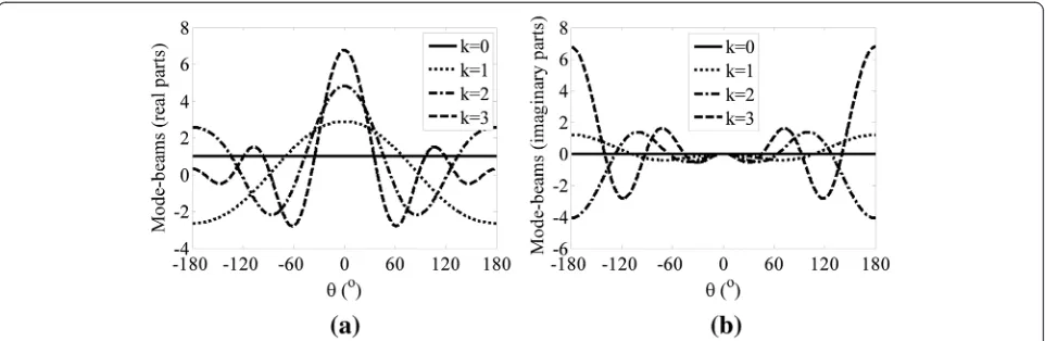
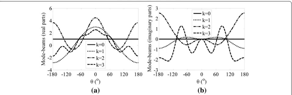
Fig. 4The 0th- to 3rd-order mode-beams of the four-sensor uniform linear array atd/λ= 0.1.aReal parts.bImaginary parts
Fig. 5Synthesized beampatterns of the four-sensor uniform linear array with the use of different models atd/λ= 0.1 and 0.3.ad/λ= 0.1.
been proven to possess the highest superdirectivity for a given number of sensors, and its DI approaches 20logN (dB) when the inter-sensor spacing becomes infinitely small [2, 23], whereNis the number of sensors. For this particular array, a difference approximation (DA) model exists [35]. It provides promising calculation accuracy when the spacing and overall length of the array are small. However, this model is difficult to implement in practice because it is highly error sensitive, which is why only first-order (vector sensor) or second-order linear arrays (at most) exist thus far. The newly developed gen-eral model should be tested if it can significantly relax restrictions on the spacing and overall size (and thus the sensor numberN).
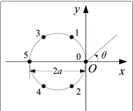
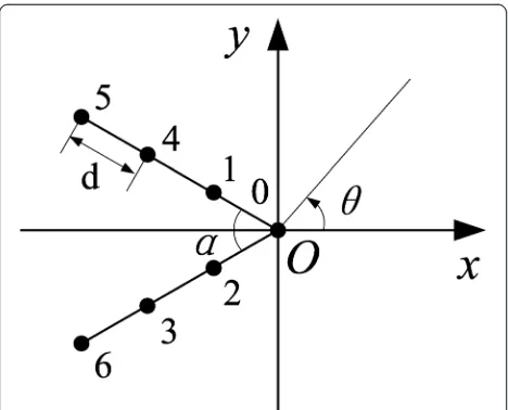
Consider an equally spaced linear array of four sen-sors, as shown in Fig. 2. From the above procedure,Ck
and λk for this four-sensor uniform linear array can be
easily derived as
Equations (34) and (35) appear to be complex, espe-cially when the order number is large. However, they are all in closed-form and can be directly calculated with the recursive formulas as ρi are given. This approach
pro-vides a practical way to obtain an accurate solution for superdirectivity. The expressions of Ck and λk with
Fig. 6Coordinates of a six-sensor uniform circular array
Fig. 7DFs and levels of robustness of the 0th- to 3rd-order modified mode-beams for the six-sensor uniform circular array.aDFs.bLevels
orders larger than 3 can be similarly derived but are not listed here for brevity.
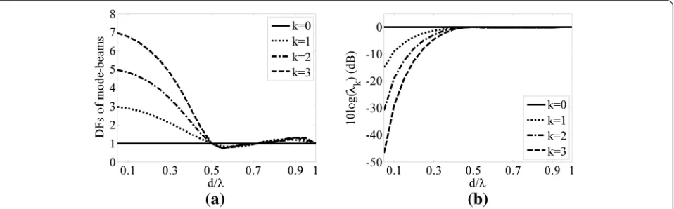
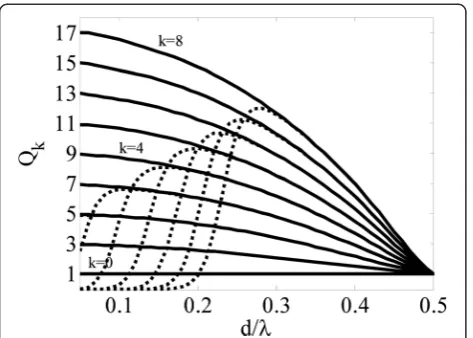
The calculated DFs and levels of robustness (10logλk) of the mode-beams are shown in Fig. 3a, b,
respectively, in which (θ0,ϕ0) = (0, 0). When d/λ< 0.5,
both the DF and the error sensitivity increase with an increase in the order number k and decrease with in-creasingd/λ. As d/λ reaches 0, the DF of thekth-order mode-beam approaches (2k+ 1), and the total DF ob-tained by summation of the 0th- to (N−1)th-order mode-beams is N2. This property is consistent with
the conclusions presented in [2] and shows significant potential in directivity improvement for linear arrays. However, the levels of robustness have no limit values and become infinite as d/λ decreases to 0. When d/λ is larger than 0.5, the DFs and levels of robustness of different mode-beams tend to be equal, and their vari-ances versus d/λ are unclear. Note that the DF and level of robustness of the 0th-order mode-beam are constant in the entire frequency band, and the values are kept at 1 and 0 dB, respectively.
Figure 4 shows the mode-beams with orders ran-ging from 0 to 3. With the geometrical symmetry considered, calculations are only performed in the xOz plane and d/λ= 0.1. The synthesized overall beampatterns are shown in Fig. 5 in which the results of different models are compared, and inter-sensor spacing is differently set. It is clear that the DA [35] and GSMDS models provide the similar main lobe width, and both of them outperform the conventional beamforming (CBF, i.e., DAS beamforming) model. However, the sidelobes of the DA model, especially the opposite beampatterns, are higher than those of the GSMDS model because the DA model involves theoretical approximations. This type of distortions increases with the increasing frequency (c.f. Fig. 5a, b). Specifically, as shown in Fig. 5b, the beampattern produced by the DA model is largely modified when d/λ= 0.3, and the opposite beampattern particularly becomes enormous. By contrast, the GSMDS model still works well.
4.2 Circular arrays
Circular arrays are desired in many circumstances because they have simple configurations, do not have left-right ambiguities, and can provide uniform beams along with 360° azimuthal directions [4, 21, 22, 37]. A six-sensor uniform circular array with radius a is
Fig. 8The 0th- to 3rd-order modified mode-beams of the six-sensor uniform circular array ata/λ= 0.1.aReal parts.bImaginary parts
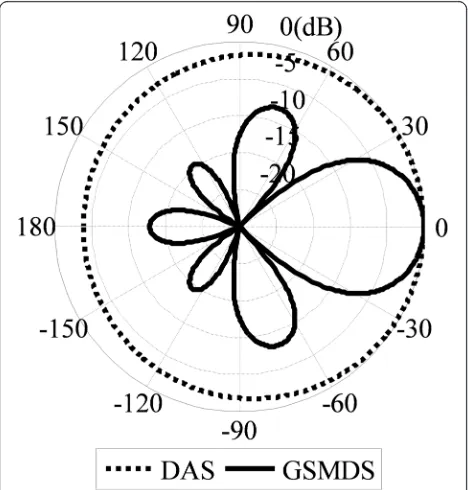
Fig. 9Synthesized superdirective beampattern (DI = 10.75 dB) of the
considered, and its coordinates are shown in Fig. 6. The origin is deliberately not located at the center of the circle for the convenience provided in the decompos-ition and synthesis procedure. The numbers adjacent to the sensors in Fig. 6 indicate the processing order of GS transformation. The DFs and levels of robustness of all mode-beams can then be readily calculated with the use of Eqs. (23) and (22). However, an additional process is needed to clearly show the regularity of the GSMDS model for circular arrays. WhenNis even, the mode-beams, DFs, and robustness parameters can be modified with the use of Eqs. (36) to (38):
^ bk¼
bk ðk¼0Þ;
b2k−1þb2k ðk¼1; 2; ⋯; N=2−1Þ;
b2k−1 ðk¼N=2Þ; 8
< :
ð36Þ
^ Qk¼
Qk ðk¼0Þ;
Q2k−1þQ2k ðk¼1; 2; ⋯; N=2−1Þ; Q2k−1 ðk¼N=2Þ;
8 < :
ð37Þ
ηk¼ λkðλ2k−1þλ2kÞ=2 ððkk¼¼10;Þ;2; ⋯; N=2−1Þ; λ2k−1 ðk¼N=2Þ;
8 < :
ð38Þ
and when N is odd, the following equations are obtained:
^ bk¼
bk ðk¼0Þ;
b2k−1þb2k ðk¼1; 2; ⋯; ðN−1Þ=2Þ;
ð39Þ
^ Qk¼
Qk ðk¼0Þ;
Q2k−1þQ2k ðk¼1; 2; ⋯; ðN−1Þ=2Þ;
ð40Þ
ηk¼
λk ðk¼0Þ;
λ2k−1þλ2k
ð Þ=2 ðk¼1; 2; ⋯; ðN−1Þ=2Þ:
ð41Þ
These equations are reasonable because of the sym-metry between the (2k−1)th and (2k)th sensors, which is also utilized in [21]. Therefore, the total number of mode-beams will decrease to (N/2 + 1) (for even N) or (N+ 1)/2 (for odd N) from N. The final synthesized beampattern and the total DF are unaffected by this modification, but the levels of robustness should be properly evaluated to keep them meaningful. The values ofλ2k−1andλ2khave the same order of magnitude, and
this means that the (2k−1)th- and (2k)th-order mode-beams have similar robustness. At this point, their
Fig. 10Coordinates of a seven-sensor V-shaped array
Fig. 11DFs and levels of robustness of the 0th- to 3rd-order modified mode-beams for the seven-sensor V-shaped array.aDFs.bLevels
average valueηkis selected to measure the robustness of
thekth-order modified mode-beam.
The DFs and levels of robustness of the modified mode-beams are shown in Fig. 7a, b, respectively, and they depict the same behavior as that of linear arrays whena/λis small. Specifically, the larger the order num-ber, the higher is the DF of this mode-beam, and the worse is the robustness. As a/λ decreases, the DF also increases, and the mode-beam becomes error sensitive. When a/λ is large, the levels of robustness almost overlap with one another, but the DFs become irregular.
The 0th-order modified mode-beam still has a constant DF and robustness in the entire frequency band.
The 0th- to 3rd-order modified mode-beams for this six-sensor uniform circular array at a/λ= 0.1 are shown in Fig. 8. Unlike the eigen-beams shown in [21], the imaginary parts of these mode-beams cannot be ignored (see Fig. 8b). As shown in Fig. 9, the synthesized final superdirective beampattern using all mode-beams is ac-tually the same as the final result using all eigen-beams in [21], which shows apparent performance improve-ment compared with the conventional DAS beampat-tern. Note that the EBDS model appears to be simpler for circular arrays than the GSMDS model, but it cannot be applied to other arrays. The superiority of the GSMDS model over the EBDS one is clear.
4.3“V”-shaped arrays
The V-shaped arrays have good potential to be used in practical applications, such as in underwater acoustic communication and navigation systems for small au-tonomous vehicles. They can also effectively show the advantages of the GSMDS model. A seven-sensor V-shaped array is shown in Fig. 10. It consists of two four-sensor uniform linear arrays with a common four-sensor. These two linear arrays are axisymmetric with respect to thex-axis. The opening angleαis set to 60°.
The DFs and levels of robustness shown in Fig. 11a, b, respectively, were modified with the use of Eqs. (40) and (41), respectively, and the number of mode-beams was changed to four. Note that the DFs do not regularly change with d/λ or the order number, but the levels of robustness still show the same behavior as those of the linear and circular arrays. Figure 12 shows the 0th- to 3rd-order modified mode-beams for the seven-sensor V-shaped array atd/λ= 0.1. The synthesized superdirective beampattern using these mode-beams is compared with
Fig. 12The 0th- to 3rd-order modified mode-beams of the seven-sensor V-shaped array atd/λ= 0.1.aReal parts.bImaginary parts
Fig. 13Synthesized superdirective beampattern (DI = 10.39 dB) of
the conventional DAS beampattern in Fig. 13. The per-formance enhancement is also clear.
These analyses indicate that the GSMDS model can accurately decompose the optimal solutions of superdir-ectivity into different sub-solutions for arrays of different shapes. When it is applied to the above three array types (not limited to these arrays), the robustness property of the mode-beams with high orders clearly becomes error sensitive. Therefore, the reduced-rank technique can be readily used to synthesize robust high-order superdirec-tive beampatterns.
5 Comparisons with the DAS and MVDR methods
Some detailed comparisons between the GSMDS method and some widely used methods are presented in the fol-lowing simulations, so that the advantages of the proposed method will be clearer.
We regard a nine-sensor linear array as an example. The sensor gain and phase errors, termed g and ψ,
respectively, are assumed to be statistically independent, zero mean, Gaussian random variables, and their vari-ances are set toσ2
g ¼σ2ψ ¼10−6.
The average values of actual DFs of the mode-beams calculated using Eq. (32) are shown in Fig. 14 (dotted lines), in which the different mode-beams show differ-ent sensitivities to errors at this level of errors. Specif-ically, the mode-beams with orders lower than 3 are all sufficiently robust. Their average DFs show no changes in the given frequency band, whereas the average DFs of the 3th- to 8th-order mobeams de-crease at some frequencies, called “critical frequen-cies”. The smaller the order, the lower is the critical frequency. This is because the lower-order mode-beams correspond to smaller frequencies when the re-quired robustness level is the same, as shown in Fig. 3b. It is clear that the high-order mode-beams in Fig. 14 do not contribute to the total DF in some fre-quency ranges, and these mode-beams can be trun-cated, leading to the improved robustness. If better superdirectivity is required to be obtained in practice, the maximum order of the retained mode-beams is unnecessarily selected to be large.
Fig. 14Theoretical (solid line) and average (dotted line) DFs of mode-beams for the nine-sensor linear array
Fig. 15DIs of different methods for the nine-sensor linear array
Fig. 16Average DIs of different methods for the nine-sensor linear
array
Fig. 17Experimental uniform linear array of nine omnidirectional
The average DIs of this array achieved using differ-ent methods are shown in Fig. 15 by considering the same level of errors ( σ2
g ¼σ2ψ ¼10−6 ). The DAS method is the most robust method, but its directivity is the lowest. By contrast, the minimum variance dis-tortionless response (MVDR) method can provide the highest directivity, but its robustness is the worst. The average DI of the MVDR method degrades at approxi-mately d/λ= 0.26 and is even less than that of the DAS method when d/λ< 0.19.The theoretical DI of the GSMDS method without any errors, which is obtained by summing the theoretical DFs of mode-beams shown in Fig. 14, is equal to that of the MVDR method. Fur-thermore, at d/λ= 0.26, the average DI of the GSMDS method, which is achieved by summing the average DFs of mode-beams in Fig. 14, starts to decrease but with a slower velocity. Compared with the MVDR method, the achieved average DI of the GSMDS method can reach 16.3 dB at d/λ= 0.19, which is also
higher than that of the DAS method. When the fre-quency is lower, the DI of the GSMDS method is still larger than that of the DAS and MVDR methods owing to the contribution of the robust lower-order mode-beams.
6 Comparisons with the regularization-based methods
As presented previously, the type of regularization-based methods, specifically the DL method, is exten-sively used in practice and can be selected as a typical example to compare with the proposed method. The average DIs obtained using these two methods are shown in Fig. 16.
It is observed that the average DI of the DL method is larger than that of the MVDR method in the low-frequency band, which indicates that adding a regularization param-eter (i.e., DL value) effectively improves robustness. How-ever, if the selected regularization parameter is large, then the beamformer is over-robust and the DI is theor-etically low. If the regularization parameter selected is small, then robustness is not sufficiently good to lead to an exceedingly low actual DI. In Fig. 16, the average DIs of DL = 10−2(large) and DL = 10−8(small) in the low-frequency range are lower than those of the GSMDS method, whereas the obtained DI for DL = 10−6is larger than that of the GSMDS method. It is clear that the regularization-based methods will perform better than the GSMDS method when the regularization parameter is appropriately selected (e.g., DL = 10−6 in this ex-ample), but the appropriate parameter is not easily de-termined in many practical applications because the level of actual errors is always unknown so that the final results will be always degraded in some frequency bands. By contrast, the performance of the GSMDS
Table 1Performance measures of practical beampatterns
Method DI (dB) HPBW (°) SL (dB)
f= 1350 Hz (d/λ= 0.09)
DAS 5.80 118.74 −12.46
GSMDS (K= 3) 11.92 48.05 −12.98
f= 3000 Hz (d/λ= 0.2)
DAS 8.63 80.70 −9.99
GSMDS (K= 6) 15.01 31.41 −14.00
f= 5000 Hz (d/λ= 0.33)
DAS 11.07 59.50 −11.65
GSMDS (K= 8) 15.57 28.68 −14.16
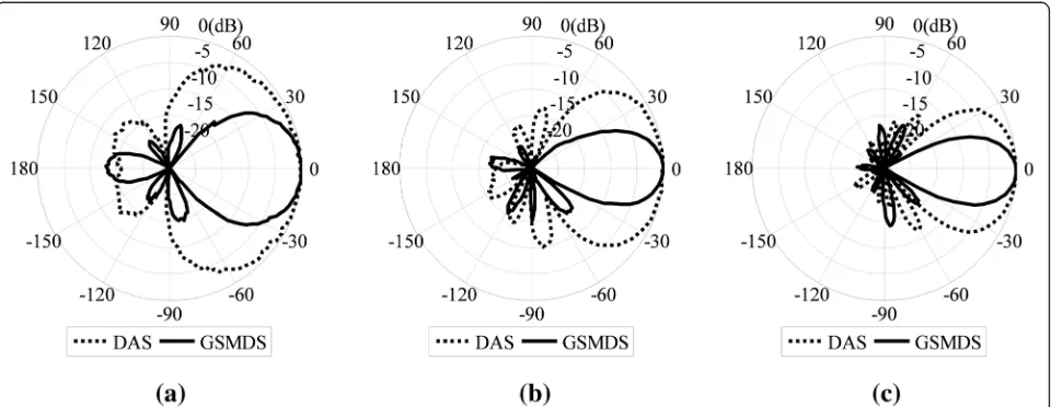
Fig. 19Synthesized experimental superdirective beampatterns for the nine-hydrophone linear array compared with conventional DAS
method is determined when the actual level of errors is given, and it will not change with other parameters. In other words, although the regularization-based methods can work better than the GSMDS method, they also have the great possibility to give worse re-sults in some frequency ranges over the proposed method in practical applications. For a conservative purpose, the GSMDS method will be preferred to be applied in practice because it has the determined per-formance and takes no risks of giving worse results in comparison with the regularization-based methods.
7 Experimental results
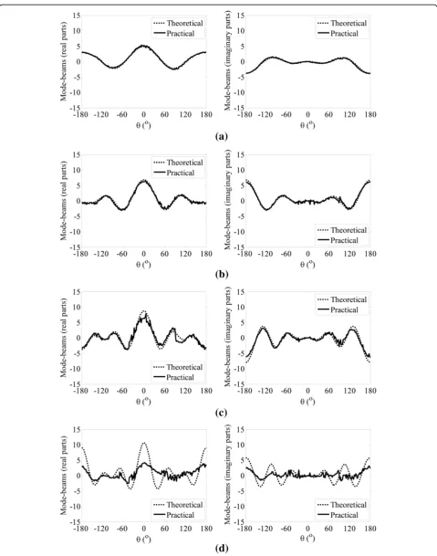
An experimental uniform linear array consisting of nine omnidirectional hydrophones was prepared. This array is shown in Fig. 17, and the inter-sensor spacing is 10 cm. The data acquired in an anechoic water tank were used for experimental verification. The signals employed in the experiment were rectangular-window-modulated single-frequency continuous-wave pulses, and their frequencies were 5000, 3000, and 1350 Hz. Figure 18 shows the theoretical and practical mode-beams with orders ranging from 2 to 5 at a frequency of 1350 Hz (d/λ= 0.09). The mode-beams with orders smaller than 4 clearly agree well with the corresponding theoretical ones. Because of the errors from hydrophone gain and phase mismatches, sensor position perturba-tions, and structural scattering, all the high-order mode-beams are corrupted, and distortions increase with an increase in the order number. This condition is consist-ent with the above-presconsist-ented analyses on λk. Although
the 0th- and 1st-order mode-beams, as well as the 6th-to 8th-order ones, are not shown here, their properties are self-evident. The mode-beams at 3000 Hz (d/λ= 0.2) and 5000 Hz (d/λ= 0.33) also exhibit similar behavior, but they are not shown here for brevity.
The above analyses indicate that the overall practical beampatterns at these three frequencies can be easily synthesized. Figure 19 shows these superdirective beam-patterns, and Table 1 lists their performance measures, including DIs, half-power beamwidths (HPBWs), and sidelobe levels (SLs). The DI values were calculated with the assumptions that the beampatterns had rotational symmetry, and the noise field was isotropic. The SL was defined as the maximum level of sidelobes. The fre-quency is 1350 Hz, so the practical mode-beams with orders larger than 3 are unusable because of their error sensitivities. Therefore, a reduced-rank beampattern is synthesized with the use of only the 0th- to 3rd-order mode-beams (K= 3). The measured SL is almost the same as the conventional DAS beampattern, but the HPBW decreases to 48.05° unlike the conventional DAS beamwidth at approximately 118.74°. Because the main lobe is pointed toward the endfire direction, the DF is
improved by approximately a factor of four in this par-ticular case and 6 dB for the DI. For high frequencies, e.g., 3000 Hz, the 4th- to 6th-order mode-beams (K= 6) are also usable, and the DI of the final superdirective beampattern is improved by approximately 6 dB over its conventional DAS counterpart. When the frequency increases to 5000 Hz, all mode-beams (K= 8) are ro-bust against errors and can be used to synthesize the superdirective beampattern. However, the DI enhance-ment is approximately 4.5 dB, which is smaller than those in the two above cases. Both the superdirective beampatterns have lower SLs and narrower HPBWs than the conventional DAS beampatterns when the frequencies are 3000 and 5000 Hz, a result indicating better performance over the DAS method.
It is found that the effect of actual errors on mode-beams for this experimental linear array is similar to that shown in Fig. 14, although the actual errors of the experimental linear array are not only from the sensor gain and phase. Accord-ing to the analyses in the“Comparisons with the DAS and MVDR methods” section, the average DFs of mode-beams with orders smaller than 4 show good performance at 1350 Hz (d/λ= 0.09), meaning the appropriate maximum order is 3 at this level of errors. From Fig. 14, it is also in-ferred that the appropriate maximum order will be 5 and 8 when the frequencies are 3000 Hz (d/λ= 0.2) and 5000 Hz (d/λ= 0.33), respectively, if the actual errors are inde-pendent of the frequency. The conclusions for the cases at 1350 Hz (d/λ= 0.09) and 5000 Hz (d/λ= 0.33) are approximately right, whereas the case at 3000 Hz (d/λ= 0.2) shows some deviations in experimental re-sults because of effects of other errors.
As presented previously, the highest order of satisfac-tory mode-beams has to be selected with special atten-tion, and this selection deserves a final consideration. If the level of actual errors of a practical array can be precisely estimated, then the highest order can be easily determined with the use of computer simulations, and the truncation of unsatisfactory high-order mode-beams can be conveniently conducted. When the information of actual errors cannot be known, an ad hoc experimen-tal measurement is required to determine the highest order, which can also be effectively used during trunca-tion, as is the case in this study.
8 Conclusions
involved in this model, meaning this model provides an effective mechanism to achieve high-order superdirectiv-ity. The beamforming process is simplified by decom-position of the optimal beampattern and maximum DF into mode-beams and their associated DFs to signifi-cantly facilitate the implementation of superdirectivity. All of these results are directly derived from the optimal solutions of superdirectivity, so the GSMDS method can be applied to sensor arrays with arbitrary geometries, and no a priori knowledge of errors are required. Design examples for three different arrays show that as the order number increases, the robustness of mode-beams decreases. Therefore, robust superdirective beampatterns should be synthesized with the use of a reduced-rank treatment. The performance of this technique is demon-strated with simulations and real-data experiments. Fur-ther work can focus on the error control for high-order mode-beams to further improve the practically achiev-able superdirectivity. An in-depth study of applying this model to other complex arrays, such as volumetric ar-rays, will also be a main topic in the further.
Competing interests
The authors declare that they have no competing interests.
Acknowledgements
This work was supported by the National Natural Science Foundation of China (Grant Nos. 11274253 and 60901076) and the Fundamental Research Funds for the Central Universities (Grant No. 3102014JCQ01008).
Received: 9 February 2015 Accepted: 14 July 2015
References
1. HL Van Trees,Optimum Array Processing: Part IV of Detection, Estimation, and Modulation theory(John Wiley & Sons, Inc, New York, 2002), pp. 59–71. 274–289, 439–443
2. AI Uzkov, An approach to the problem of optimum directive antenna design. Compt. Rend. Acad. Sci. U.R.S.S.53, 35–38 (1946)
3. JB Franklin,Superdirective Receiving Arrays for Underwater Acoustics Application
(Defence Research Establishment Atlantic, Dartmouth, Nova Scotia, 1997) 4. Q-C Zhou, H Gao, H Zhang, F Wang, Robust superdirective beamforming for
HF circular receive antenna arrays. Prog. Electromagn. Res.136, 665–679 (2013) 5. E Shamonina, L Solymar, Maximum directivity of arbitrary dipole arrays.
IET Microwaves, Antennas Propagation9, 101–107 (2015)
6. R Berkun, I Cohen, J Benesty, Combined beamformers for robust broadband regularized superdirective beamforming. IEEE/ACM Trans. Audio Speech Lang. Process.23, 877–886 (2015)
7. BD Carlson, Covariance matrix estimation errors and diagonal loading in adaptive arrays. IEEE Trans. Aero. Elec. Sys.24, 397–401 (1988) 8. H Cox, R Zeskind, M Owen, Robust adaptive beamforming. IEEE Trans.
Acoust. Speech Signal Process.35, 1365–1376 (1987)
9. MR Bai, C-C Chen, Regularization using Monte Carlo simulation to make optimal beamformers robust to system perturbations. J. Acoust. Soc. Am. 135, 2808–2820 (2014)
10. S Doclo, M Moonen, Design of broadband beamformers robust against gain and phase errors in the microphone array characteristics. IEEE Trans. Signal Process.51, 2511–2526 (2003)
11. M Crocco, A Trucco, The synthesis of robust broadband beamformers for equally-spaced linear arrays. J. Acoust. Soc. Am.128, 691–701 (2010) 12. A Trucco, M Crocco, Design of an optimum superdirective beamformer
through generalized directivity maximization. IEEE Trans. Signal Process. 62, 6118–6129 (2014)
13. S Doclo, M Moonen, Superdirective beamforming robust against microphone mismatch. IEEE Trans Audio Speech Lang Process15, 617–631 (2007)
14. M Crocco, A Trucco, Design of robust superdirective arrays with a tunable tradeoff between directivity and frequency-invariance. IEEE Trans. Signal Process.59, 2169–2181 (2011)
15. A Trucco, F Traverso, M Crocco,Robust superdirective end-fire arrays
(Proceedings of OCEANS 2013, Bergen, Norway, 2013), pp. 1–6
16. H Cox, RM Zeskind, T Kooij, Practical supergain. IEEE Trans. Acoust. Speech Signal Process.34, 393–398 (1986)
17. DJ Schmidlin, Directionality of generalized acoustic sensors of arbitrary order. J. Acoust. Soc. Am.121, 3569–3578 (2007)
18. BA Cray, AH Nuttall, Directivity factors for linear arrays of velocity sensors. J. Acoust. Soc. Am.110, 324–331 (2001)
19. BA Cray, VM Evora, AH Nuttall, Highly directional acoustic receivers. J. Acoust. Soc. Am.113, 1526–1532 (2003)
20. GL D’Spain, JC Luby, GR Wilson, RA Gramann, Vector sensors and vector sensor line arrays: comments on optimal array gain and detection. J. Acoust. Soc. Am.120, 171–185 (2006)
21. YL Ma, YX Yang, ZY He, KD Yang, C Sun, YM Wang, Theoretical and practical solutions for high-order superdirectivity of circular sensor arrays. IEEE Trans. Ind. Electron.60, 203–209 (2013)
22. Y Wang, YX Yang, YL Ma, ZY He, Robust high-order superdirectivity of circular sensor arrays. J. Acoust. Soc. Am.136, 1712–1724 (2014) 23. AT Parsons, Maximum directivity proof for three-dimensional arrays.
J. Acoust. Soc. Am.82, 179–182 (1987)
24. M Uzsoky, L Solymar, Theory of super-directive linear arrays. Acta Phys. Acad. Sci. Hungary6, 185–205 (1956)
25. RJ Urick,Principles of underwater sound(McGraw-Hill, New York, 1983), p. 42 26. F Ling, D Manolakis, JG Proakis, A recursive modified Gram-Schmidt
algorithm for least-squares estimation. IEEE Trans. Acoust. Speech Signal Process.34, 829–836 (1986)
27. K Gerlach, FF Kretschmer, Convergence properties of Gram-Schmidt and SMI adaptive algorithms. IEEE Trans. Aero. Elec. Sys.26, 44–56 (1990) 28. K Gerlach, FF Kretschmer, Convergence properties of Gram-Schmidt and
SMI adaptive algorithms. II, IEEE Trans. Aero. Elec. Sys.27, 83–91 (1991) 29. JN Sahalos,Orthogonal Methods for Array Synthesis: Theory and the ORAMA
Computer Tool(Wiley, London, 2006), pp. 69–72
30. S Enomoto, Y Ikeda, S Ise, S Nakamura,Optimization of Loudspeaker and Microphone Configurations for Sound Reproduction System Based on Boundary Surface Control Principle(Proceedings of the 20th
International Congress on Acoustics, ICA 2010, Sydney, Australia, 2010), pp. 1–7
31. JWR Griffiths, JE Hudson, An introduction to adaptive processing in a passive sonar system, inAspects of signal processing, ed. by G Tacconi (Springer, Netherlands, 1977), pp. 299–308. Vol. 33–1
32. SA Schelkunoff, A mathematical theory of linear arrays. Bell Syst. Tech. J. 22, 80–107 (1943)
33. RL Pritchard, Optimum directivity patterns for linear point arrays. J. Acoust. Soc. Am.25, 879–891 (1953)
34. RL Pritchard, Maximum directivity index of a linear point array. J. Acoust. Soc. Am.26, 1034–1039 (1954)
35. VF Humphrey, PC Hines, V Young, Experimental analysis of the performance of a superdirective line array, inProceedings of the Seventh European Conference on Underwater Acoustics(Delft, Holland, 2004), pp. 1033–1038 36. A Trucco, F Traverso, M Crocco, Broadband performance of superdirective
delay-and-sum beamformers steered to end-fire. J. Acoust. Soc. Am.135, EL331–EL337 (2014)