A scalable multi sink gradient based routing protocol for traffic load balancing

R E S E A R C H

Open Access

A scalable multi-sink gradient-based routing

protocol for traffic load balancing

Hongseok Yoo

, Moonjoo Shim

and Dongkyun Kim

Abstract

Wireless sensor networks have been assumed to consist of a single sink and multiple sensor nodes which do not have mobility. In these networks, sensor nodes near the sink dissipate their energy so fast due to their many-to-one traffic pattern, and finally they die early. This uneven energy depletion phenomenon known as the hot spot problem becomes more serious as the number of sensor nodes (i.e., their scale) increases. Recently, multi-sink wireless sensor networks have been envisioned to solve the hot spot problem. Gradient routing protocols are known to be appropriate for the networks in that network traffic is evenly distributed to multiple sinks to prolong network lifetime and they are scalable. Each node maintains its gradient representing the direction toward a neighbor node to reach one of the sinks. In particular, existing protocols allow a sensor node to construct its gradient using the cumulative traffic load of a path for load balancing. However, they have a critical drawback that a sensor node cannot efficiently avoid using the path with the most overloaded node. Hence, this paper

introduces a new Gradient routing protocol for LOad-BALancing (GLOBAL) with a new gradient model to maximize network lifetime.

The proposed gradient model considers both of the cumulative path load and the traffic load of the most overloaded node over the path in calculating each node’s gradient value. Therefore, packets are forwarded over the least-loaded path, which avoids the most overloaded node. In addition, it is known that assigning a unique address to each sensor node causes much communication overhead. Since the overhead increases as the network scales, routing protocols using an address to indicate the receiver in forwarding a packet are not scalable. Thus, GLOBAL also includes an addressing-free data forwarding strategy. Through ns-2 simulation, we verify that GLOBAL achieves better performance than the shortest path routing and load-aware gradient routing ones.

Keywords:Wireless sensor networks (WSNs), multi-sink, load balancing, gradient, routing

I Introduction

Traditionally, wireless sensor networks (WSNs) are com-posed of a large number of sensor nodes and a single sink. Since the distance from each sensor node to a sink (except one-hop neighbor nodes of the sink) is larger than the transmission range of sensor nodes, sensor nodes should transmit their data packet to the sink in a multi-hop manner. Therefore, sensor nodes near the sink tend to dissipate their energy faster than nodes located far away from the sink because they have to forward a large number of data. This uneven energy depletion, known as the hot spot problem [1], drastically reduces

the lifetime of sensor networks. In addition, as the net-work scales in terms of the number of sensor nodes, the hot spot problem becomes more serious. Particularly, the WSN architecture with a single sink which creates a many-to-one traffic pattern is considered as the major cause of the hot spot problem [2].

The deployment of multiple sinks might be able to pro-vide a solution to overcoming the architectural limitation of the WSN with a single sink [3]. However, deploying more sinks simply is not enough to solve the problem. We need to design novel communication protocols to realize potential benefits of the multi-sink architecture. When the network traffic is evenly distributed among the multiple sinks, the hot spot problem is expected to be significantly alleviated. Therefore, an efficient routing protocol is required to load balance network traffic * Correspondence: dongkyun@knu.ac.kr

2

School of Computer Science and Engineering, College of IT Engineering, Kyungpook National University, Daegu, Korea

Full list of author information is available at the end of the article

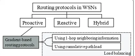
evenly among the multiple sinks (load-balancing func-tionality), because the direction of traffic flows is directly determined by the routing protocol. Particularly, in large-scale WSNs, communication protocols should large-scale with the number of sensor nodes [4]. Routing protocols pro-posed in the literature for WSNs can be categorized in different ways. Depending on the fashion in which rout-ing paths are established, they can be broadly classified into three classes as shown in Figure 1 [5]: (1) proactive, (2) reactive, and (3) hybrid protocols. In proactive proto-cols, every route is computed in advance, regardless of the need of packet delivery. On the other hand, reactive protocols allow routes to be computed on demand. Hybrid protocols combine properties of both proactive and reactive protocols. Among those protocols, it is known that gradient-based routing protocols which belong to the proactive protocols are scalable, because they are not required to maintain information about net-work topology [6]. Therefore, we favor a gradient-based routing approach for the large-scale WSNs with multiple sinks. We attempt to mitigate the hot spot problem through load-balancing functionality.

In gradient-based routing protocols, the gradient is defined as the minimum cumulative link (or node) cost along the path, which will be used to transmit its data to the sink. Data from a sensor node flow toward only neighbor nodes having lower gradient. All the gradients of the network nodes create their gradient field whose lowest value the sink has in order to make data always flow toward the sink. The link (or node) cost can take different forms such as hop count, energy consumption, or physical distance, depending on routing design objectives.

Until now, several gradient-based protocols have been proposed to achieve such load balancing [6-11]. They can be categorized into two classes as shown in Figure 1: (a) protocols that exploit the traffic load information of a forwarder’s 1-hop neighbor nodes, and (b) protocols that utilize the cumulative traffic load information of sensor nodes over a path from a sensor node to the sink. In the first class, the link cost is defined as the amount of energy consumption or the hop count when establishing the

gradient field. Data packets are transmitted along the energy-efficient path to the sink or the path with the minimum end-to-end delivery latency from sensor nodes to the sink. Considering the remaining energy or the queue length of the forwarder’s 1-hop neighbor nodes, the neighbor nodes with heavy traffic load or low residual energy are prevented from being selected as a next for-warder, based on their customized forwarding rules. In these protocols, however, sensor nodes cannot spread the traffic evenly since there is no way for them to get the information about heavily loaded region (i.e., hot spot regions near the sinks) several hops away from them [12]. In the second class, each sensor node constructs its gradient using the cumulative traffic load informationa of the path potentially used for its data delivery. Then, data flow through the least-loaded path over the estab-lished gradient field. Unlike the first class protocols that utilize local information, they can spread the traffic to perform the load balance since they use the cumulative path load. However, they have some drawbacks that a sensor node cannot efficiently avoid using the path with the most overloaded node among its all possible paths since only the cumulative path load is not enough to identify the path including the most overloaded node [13]. We focus on overcoming this drawback in this work.

Based on the above observation, this paper introduces a new gradient-based routing protocol for LOad-BALancing (GLOBAL) in large-scale WSNs with multiple sinks. Assuming that network lifetime is defined as the time elapsed from the deployment to the instant when one of sensor nodes becomes dead, the network lifetime is lim-ited by the lifetime of the most over-loaded sensor node. Therefore, the routing protocol should be able to prevent sensor nodes from using a path including the most over-loaded sensor node. In GLOBAL, in order to allow a sensor node to use the least-loaded path which also avoids the most overloaded sensor node, each sensor node calcu-lates its gradient using the weighted average (WA) of the cumulative path load and traffic load of the most over-loaded node over the path. The WA technique is a well-known method used to create a new metric as in [14]. In WA, weights are selected heuristically to obtain overall performance improvements. GLOBAL also includes a heuristic method to determine our weight values.

Generally, an address is used to indicate the receiver in forwarding a packet. Hence, each sensor node should be assigned to its unique address prior to network operations. Such addressing can be made in manufacturing sensor nodes. Since duplicate addresses can exist in the network due to a lot of addressing errors in manufacturing sensor nodes, an automatic addressing protocol is needed to assign a unique address to each node in the network. How-ever, this protocol has much communication overhead as Gradient-based

well as much energy consumption. In particular, the over-head increases as the network scales. Hence, in gradient routing protocols, a gradient value is simply included in the packet and only neighbor nodes with smaller gradients participate in forwarding the packet. Due to the existence of multiple neighbor nodes with smaller gradients, dant packet forwarding can occur. Although such redun-dancy improves reliability, it needs to be suppressed, depending on routing design objectives [15]. GLOBAL, therefore, has an addressing-free data forwarding strategy without such overhead and redundancy.

The rest of the paper is organized as follows. We intro-duce related works on gradient-based routing protocols with load balance and their general operations in Section II. Section III presents the detailed description for the proposed GLOBAL protocol. Section IV presents the results of the performance evaluation of the proposed scheme and discusses the impact of different values of the simulation parameter on the performance of GLO-BAL. Finally, we conclude this paper with future work in Section V.

II Related works

A General operation of gradient-based routing protocols

In gradient-based routing protocols, no routes are set up prior to sending data. Nodes are assigned only gradients, which are equal to the minimum cumulative link (or node) cost to reach the sink. When a sensor node has some data packets to send, it broadcasts its data packet with its own gradientG. Only its neighbor nodes with gradients lower thanGparticipate in rebroadcasting the packet. Gradients of sensor nodes create a gradient field whose lowest value the sink has so that the data packets always flow toward the sink.

A straightforward solution to setting up the gradient field would be found through flooding. Initially, each sen-sor node sets its gradient to infinity. After the sink broad-casts an ADV (advertisement) packet containing its own gradient 0, the packet propagates throughout the net-work. Upon receiving the ADV packet from node M, node N acquires a path with gradientGM+CN, where GMis node M’s gradient andCNis the link cost from N to M. The node N then compares its current gradientGN andGM+CN. If the new gradient is smaller than the old

one, it sets GN to GM + CN and broadcasts an ADV

packet with an inclusion of its new gradient. Whenever a sensor node receives an ADV packet with gradient smal-ler than its current gradient, it updates its gradient accordingly and broadcasts a new ADV packet.

B Gradient-based routing protocols with load balancing

In this section, two classes of existing gradient-based rout-ing protocols with load balancrout-ing which are mentioned in

Section I are described in more detail. We briefly review representative protocols belonging to each class.

B.1 Using 1-hop neighboring information

Huang et al. [6] proposed the SGF protocol. Since SGF aims to route data along an energy-efficient path to the sink, energy consumption is used as link cost for estab-lishing a gradient of each sensor node. Assuming that the transmission power of sensor nodes is adjustable, each sensor node (say node i) measures the actual channel gainδijbased on its transmission power and received power of a control packet (i.e., ADV packet) sent by its neighbor node (say nodej) and calculates the minimum transmission power required to send data from nodeito nodej, fromδij.

In order to balance network traffic load, SGF intro-duces a new forwarding method that gives sensor nodes with more remaining energy more chance to forward their neighbor nodes’packets. Hence, nodeitransmits its data with its gradient, and then, when nodejreceives a packet from its neighboring node i, nodejdetermines whether to forward the received packet, based on its resi-dual energy as well as gradients of nodeiand itself. Some protocols are similar to SGF (see [7,8]).

B.2 Using cumulative path load

Lie et al. [9] proposed the PWave protocol, which takes its inspiration from potential theories and principles in resis-tive electric networks. In PWave, a gradient field is con-structed in a WSN and routing is determined by the gradients of nodes just like the way that an electric current flows in a resistive electric network. The sink’s gradient is set to 0, and the others’gradients are assigned to minimize a certain global objective function. Data can only flow from each sensor node toward its neighbor nodes having lower gradients than it has. As stated in [9], by minimizing the global objective function, PWave yields a multi-path proportional routing scheme where the sensor node spreads its traffic across multiple paths inversely propor-tional to the cumulative path cost. The cumulative path cost is defined as the sum of link costs along the path.

node. Similar approaches based on the cumulative path load are founded in [10,11].

III GLOBAL: a gradient-based routing protocol for LOad-BALancing

The proposed GLOBAL protocol is designed under the following assumptions.

•Types of traffic: In our target applications, both per-iodic traffic and aperper-iodic event-driven traffic are generated from sensor nodes.

• Position of sinks and sensor nodes: The sinks and sensor nodes are randomly placed, and all sinks and sensor nodes have no mobility.

• Communication ranges: The fixed and

homoge-neous transmission range is set, and the carrier sen-sing, interference range is two times larger than the transmission range.

•Security concern: As stated in [16], since the hard-ware of sensor nodes is not tamper-resistant, the attacker can control any sensor node through physi-cal compromise and it can also acquire the secret keys to participate in legitimate inter-node communi-cations. Even though some cryptographic protocols can be applied to inter-node communications, the attacker can still access the cryptographic keys through physical compromise in order to participate in the communications in a legitimate way. After get-ting control of a sensor node, the attacker can force some sensor nodes to perform malicious attacks (i.e., altering/dropping the messages which should be for-warded to the next-hop node). In this current version of GLOBAL, the countermeasure for such attacks are not included, since security issues are beyond the scope of this work.

The GLOBAL protocol consists of three phases: gradi-ent field establishmgradi-ent, data forwarding, and gradigradi-ent field maintenance phases. In the gradient field establish-ment phase, sinks flood an ADV packet. In receiving an ADV packet, a senor node calculates its gradient using the information specified in the received ADV packet. In the data forwarding phase, an address is useless to indi-cate the receiver in forwarding a packet. When a sensor node updates its gradient, it acquires the gradient value of its next-hop node. Hence, the gradient value can be used as the next-hop node identifier. In the gradient field maintenance phase, since the traffic load distribution of sensor nodes changes dynamically after sensor nodes start to transmit their data, each sensor node refreshes its gradient whenever it overhears a periodic data packet from its neighbor nodes. The periodic data packet includes the information required to calculate the gradi-ent value. In the rest of this section, we first introduce

the proposed cost & gradient models and then present the detailed description of each phase in the proposed GLOBAL protocol.

A The proposed cost & gradient models

A.1 The cost model

The link (or node) cost that is used to evaluate routes is a very important component of the gradient-based rout-ing protocols. For load balancrout-ing, GLOBAL uses traffic load of sensor nodes as cost for gradient construction (Detailed mechanisms of gradient construction are given in the next subsection). Different from the value which is defined at the link level such as the amount of energy consumed in transmitting a packet and the geographical distance between sensor nodes, a traffic load is the cost defined at the node level.

As indicated in [17], the traffic loadTLiin each sensor node (say nodei) is defined as the sum of the traffic pas-sing through nodeiand the traffic passing through node i’s neighbor nodes due to the broadcast nature of radio channels. AlthoughTLican be calculated based on the actual amount of traffic, the amount of local energy dissi-pated in the radio communication can be utilized to obtain TLisince all the communication activities (transmission, reception, and overhearing) occurring at nodeiand node i’s neighbor nodes result in decrease in nodei’s residual energy [18]. In addition, let us assume that two sensor nodes (say nodesAandB) consume the same amount of energy per unit time and their energy expenditure only comes from the communication activities, but nodeBhas the larger amount of residual energy than nodeA. In this case, although they consume the same amount of energy for the communication activities, nodeAeventually dies earlier than nodeB. Therefore, a traffic load of nodeB should be estimated lower than nodeAto make other nodes favor nodeBthan nodeAas their forwarder. Based on the above observation, we use the residual energy depletion rate (REDR) as the metric that measures the traf-fic load of a given sensor node. In this work, we assume that all sensor nodes are battery powered and the amount of their energy consumed in executing activities (i.e., sen-sing) except for communication activities is identical to each other. Therefore, REDR is only affected by the energy consumption resulting from the communication activities. Hence, REDR can be substituted for traffic load.

In GLOBAL, nodeiupdates its gradient whenever it receives an ADV or a periodic data message from its neighbor nodes (Refer to following sub-sections for details). Before updating its gradient, nodeifirst updates its REDR in order to use the latest REDR information. Whenever nodeihas received the ADV or periodic data message from its neighbor nodes at timea,REDRsample_i is calculated by Equation 1, whereea_i andeb

of residual energy at timesaandb, respectively.b indi-cates the time when nodeipreviously received the ADV or periodic data message. We assume that each sensor node can measure its residual energy through a battery monitoring systemb _[19].

REDRsample_i represents the depletion rate of residual energy during the lasta - b sec-onds.

Upon obtaining a newREDRsample_i , node iupdates its residual energy depletion rate REDRithrough the well-known exponential weighted moving average method to mitigate the fluctuation ofREDRsample_i (see Equation 2). In Equation 2,REDRold

i represents the previous REDR

value of nodeiand is the smooth weighing factor.

REDRi=α·REDRoldi + (1−α)·REDR

sample

i (2)

To better reflect the current status of energy dissipa-tion of sensor nodes, we give higher weight to the new REDRsample_i by setting a to 0.3. Although sensor nodes do not have data to relay, they have to send packet peri-odically. Therefore, an initial value of REDRi is taken according to the amount of periodic data at the nodei. A.2 The gradient model

GLOBAL allows sensor nodes to set their gradients with two design goals as follows.

• Sensor nodes should favor a path which is less loaded.

• Sensor nodes should avoid a path including the most overloaded sensor node.

If only the first design goal is considered, the gradient of node i(denoted by Gi) should be set to the sum of the REDR values of the sensor nodes, which constitute the path potentially used for data delivery. Therefore, assuming that the path of node iconsists of n sensor nodes including node i,Gi is calculated by Equation 3, where REDRjis the REDR value of thejth sensor node over the path. However, with the gradient model driven by Equation 3, a sensor node cannot efficiently avoid using the path with the most overloaded node among its all possible paths since only the cumulative path load is not enough to identify the path including the most overloaded node [13]. Thus, Equation 3 should be revised to achieve the above two goals.

Gi= n

j=1

REDRj (3)

If Gi is calculated by Equation 4, sensor nodes can avoid the path including the most overloaded node. However, max1≤j≤nREDRjdoes not increase as the path has more hops. Hence, it is not an useful gradient value as explained in Section II.A. Therefore, in order to meet the two design goals, we attempt to combine the desir-able properties of the two values obtained by Equations 3 and 4. Therefore, their weighted average is taken by adopting the method introduced in [14]. See Equation 5.

Gi= max

1≤j≤nREDRj (4)

Assuming that REDRnis max1≤j≤n REDRj, Equation 5 can be changed to Equation 6. Consequently, Gi indi-cates the weighted sum of the REDR values of the sen-sor nodes which constitute the path. The REDR of the most overloaded sensor node is weighted differently from the REDRs of the other sensor nodes over the path, according to Equation 6.

Gi=β

In Equations 5 and 6, bis a weighting factor of both parameters and ranges between 0 and 1. In Section IV. B, we will investigate the impact ofbon the GLOBAL’s performance using ns-2 simulation and introduce a new heuristic method to choose b, based on observations from simulation results.

B Gradient field establishment

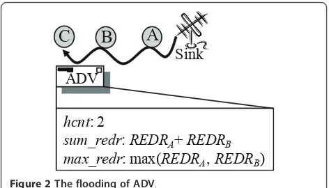
GLOBAL utilizes the naive flooding-based gradient field establishment algorithm to set up initial gradients of sensor nodesc_{. When a network is initialized, each of} sinks floods an ADV packet one after another with a pre-defined time interval, which is set to enough time to ensure that two consecutive floodings do not interfere with each other. The ADV packet contains the following three fields for the gradient field construction. Initially, sinks have the three fields whose values are 0. For example, in Figure 2, when sensor node B rebroadcasts

the ADV packet received from sensor node A, hcnt,

sum_redr, andmax_redrcarry 2, REDRA +REDRBand max(REDRA, REDRB), respectively. REDRA and REDRB represent the REDR values of sensor nodes A and B, respectively.

• sum_redr: The sum of REDR values of sensor nodes that the ADV packet has traversed.

• max_redr: The maximum REDR value among

REDR values of sensor nodes that the ADV packet has traversed.

When a sensor node (say nodei) initially receives an ADV packet, it firstly initializes all local variables to NULL and its local variables including its gradient are updated through the fields specified in the received ADV packet (see Algorithm 1). When nodeireceives an ADV packet for the first time, it increases the hcntvalue appeared in the ADV packet by one in order to account for the new hop distance.s_hcntkeeps the increased value (i.e.,hcnt+ 1). Since nodeiinitially does not have any path information, the newly acquired path will be used to transmit data as the shortest hop path. Hence, path_hcntis set to the same value ofs_hcnt. Both hop-count variables are used to avoid an excessive increase in the path length as followings. Then, after updating its REDRithrough the procedure described in Section III. A.1, nodeiupdatessum_redrLandmax_redrLas shown in Algorithm 1.sum_redrLandmax_redrLindicate the cumulative path load and traffic load of the most over-loaded node over the path, respectively. Using Equation 7, nodeicalculates its gradientGiand maintainsGiin its local memory.

From the proposed gradient model introduced in Sec-tion III.A.2,Giis calculated by averaging the two metrics, namelysum_redrLandmax_redrL, wherebis a weighting factor of both parameters and ranges between 0 and 1. After updating its local variables, nodeiupdates the fields in the ADV packet from its local variables as follows:hcnt =path_hcnt,sum_redr=sum_redrL,max_redr= max_-redrL. Finally, it rebroadcasts the ADV packet.

Gi=β·sum redrL+ (1−β)·max redrL (7)

After acquiring the initial path, nodeimay still dis-cover a less loaded path than the initial path when it receives a duplicate ADV packet. However, since the

latency of an end-to-end delivery increases as the number of hops in the path increases, it is not desirable to select a very long path with respect to load balancing. Therefore, GLOBAL defines a system parameterKin order to pre-vent a sensor node from selecting an extremely long path. Given paths providing lower gradients than a cur-rent gradient of nodei, GLOBAL allows nodeito desig-nate only the path whose hop count is not larger than s_hcnt+Kas its new path. To do so, when nodeireceives a duplicate ADV packet, it first calculates the gradientg of the newly discovered path after updating its REDR using Equation 8.

g=β·(sum redr+ REDRi) + (1−β)·max(max redr, REDRi) (8)

Only if g is lower thanGiand hcnt is smaller than s_hcnt+K, nodeidesignates the newly discovered path as its new path. Then, it setsgtoGiand rebroadcasts the ADV packet after updating fields in the ADV packet as mentioned before. Particularly, whenever nodeireceives a duplicate ADV packet, it updates thes_hcntvalue if hcnt of the received packet is smaller than a current s_hcntvalue - 1.

C Data forwarding with the proposed addressing-free forwarding strategy

GLOBAL includes an addressing-free data forwarding strategy. In GLOBAL, if a node (say node A) updates its gradient after receiving a packet, the node from which the packet is received should be designated as the node A’s next-hop node. Instead of using an address for for-warding packets, GLOBAL uses the gradient value as the next-hop node identifier. Suppose that a node (say

Algorithm 1Updating local variables at nodei s_hcnt: the shortest number of hops to reach a sink from node i.

path_hcnt: the number of hops of the current path which nodeitransmits data over.

sum_redrL : the sum of REDR of nodes (including node i) along the current path which node i transmits data over.

max_redrL : the maximum REDR value among

REDR values of sensor nodes (including node i) along the current path which nodeitransmits data over.

Gi: nodei’s gradient.

if(ADVis received for the first time) then s_hcnt=hcnt+ 1

path_hcnt=s_hcnt update REDRi

sum_redrL=sum_redr+ REDRi if (REDRi>max_redr)then

max_redrL= REDRi

end if

updateGi(=b·sum_redrL+ (1 -b) ·max_redrL) else if(Duplicate reception ofADV, or overhearing of a data packet)thenupdate REDRi

calculateg(= b· (sum_redr + REDRi) + (1 -b) · max(max redr, REDRi))

if(g < Gi&hcnt <(s_hcnt+K))then Gi=g

sum_redrL=sum_redr+ REDRi if(REDRi>max_redr)then

max_redrL= REDRi

nodej) had been the next-hop node of a node (say node i), based on their previous gradient values. Note that the gradient of each node can be changed over time. Hence, after nodeiacquired nodej’s gradient as its next-hop identifier, nodejshould still maintain the gradient value of which it informedieven though nodejhas a new gradient value, so that nodejcan relay the packet forwarded from nodei. In GLOBAL, each node broad-casts the packet with its current gradientGnexthop and

maintains that gradient value in local memoryGinformed.

When a node updates its gradient after receiving the packet, it usesGnexthopas the next-hop node identifer

when sending next packets. A node receiving a packet decides to forward the packet only ifGnexthopof the

received packet is equal to its localGinformedvalue.

D Gradient field maintenance

The initial gradient field becomes inaccurate, since the traffic load distribution of sensor nodes varies dynami-cally after sensor nodes start to transmit their data. In addition, some sensor nodes may fail to receive an ADV message since wireless channel is vulnerable to data loss. Therefore, they cannot calculate their gradients. This requires the gradient field to be refreshed timely in order to avoid the uneven traffic load distribution as well as to enable sensor nodes to acquire their accurate gradients.

Most of gradient routing protocols rely on the periodic flooding of ADV packet to reconfigure gradient fields [4,15]. However, since such a flooding incurs excessive packet overhead, the network becomes stressed, which is not scalable. Hence, GLOBAL has gradients to be updated during data transmissions without any depen-dency on flooding, which leads to little overhead. In our target application scenario, sensor nodes transmit data in a periodic manner. All periodic data packets include

three fields specified in the ADV packet. Whenever a sensor node (say nodei) overhears a data packet from its neighbor node except its current next-hop node (say nodej), they process the data packet just as they process a duplicately received ADV packet. In order to prevent the nodejfor designating nodeito its next-hop node, nodejdoes not update its gradient when it receives a data packet from nodei. As explained in Section III.C, each sensor node advertises its gradient value as the iden-tifier of a next-hop node (instead of address) to its neigh-bor nodes and it can also acquire a new identifier when a gradient is updated. Hence, when nodeireceives a packet from nodej, the packet should carry the gradient value of which nodej informed nodei previously in order to allow nodeito find out whether the received packet has been sent from nodejor not. Therefore, in GLOBAL, each node broadcasts its packet with the currentGinformed

value. When a sensor node receives a packet from a neighbor node, it can find out whether the received packet has been sent from its next-hop node or not by checking whether Gnexthopis equal toGinformedin the

received packet. In particular,Gnexthopof a sensor node is

set to NULL (as mentioned in Section III.B), because it cannot have the information on the current next-hop node until it receives an ADV message. Hence, a sensor node failing to receive an ADV message can acquire its gradient once it overhears a periodic data packet from its neighbor nodes.

After a senor node (say nodei) decides its path, its traf-fic load through the path keeps changing over time. Hence, nodei’s gradient should be dynamically updated accordingly. Therefore, when nodei overhears a data packet from its current next-hop node, it first checks the hop count of the path. Ifhcntis not larger thans_hcnt+ K, it updates its gradient in order to reflect the changes of traffic load over the path which it is currently using. Otherwise, nodeisets its gradient to infinity and tries to find a new path whose hop count is not larger thans_hcnt +K. In addition, when nodeifails to overhear a periodic packet from its current next-hop node (say nodej), the Gnexthopvalue maintained in nodeimay become unequal

to theGinformedvalue maintained in nodej. In this case,

nodeishould not designate nodejas its next-hop node. Thus, nodeisets its gradient to infinity and tries to find a new path when it fails to receive nodej’s periodic packet. We assume that each node knows the transmission inter-val of periodic traffic.

IV Performance evaluation

A Simulation setup

20 m. Since the hot spot problem becomes more serious as the network scales, we tested different network scales (i.e.,N= 20, 30, 40). Three sink nodes were positioned in the farthest locations among each other in the grid, and the others were configured as sensor nodes. Transmission, interference, and carrier sensing ranges were set to 35, 70, and 70 m, respectively. Each sensor node generated its periodic traffic as well as event-driven one.R% of nodes generated the event-driven traffic, and they were randomly re-selected every 10 s. We assumed that the event-driven traffic was also periodic for the simplicity of simulations, but it had shorter transmission interval. In addition, differ-entRvalues (i.e.,R= 5, 10, 15) were used to vary traffic rates.

We compared GLOBAL with two protocols, SPR (shortest-hop path routing) and CPL (cumulative path load). In SPR, each node transmits its data using the shortest path without any consideration of load balan-cing. On the other hand, in CPL, each node constructs its gradient based on the cumulative traffic load of a path. If

b is set to 1, GLOBAL works in the same as CPL.

Through performance comparisons of GLOBAL with CPL, we could observe the superiority of the proposed gradient model that allows each sensor node to calculate its gradient by considering both the cumulative path load and the most overloaded node over the path.

As an energy consumption model, we employed the energy model used in [12]. The packet transmission and reception energy consumption were set to 50 nJ *l+ 100 pJ/bit/m2*l*d2and 50 nJ *l, respectively, where each ofl-bit packets is transmitted at a distanced. From the assumption of a fixed transmission range,dwas set to 30 m. In addition, due to the broad-cast nature of the wireless channel, a sender’s neighbor nodes overhear its transmissions even if they are not its intended receivers. As mentioned in [20], a receiver cannot decide whether or not it is an intended receiver until the entire packet is received. Therefore, such overhearing causes unintended receivers to waste energy. Hence, assuming that the energy consumption caused by additional processing of the packet header is negligible, GLOBAL does not require additional energy consumption caused by over-hearing. Certainly, if the receiver has a mechanism to decode the packet header alone and then turn off the radio during the period of receiving the remaining part of the packet for an unintended recipient, the additional energy savings can be expected. However, such sophisti-cated scheduling comes from a high price in terms of hardware complexity and may induce delays in proces-sing at higher layers. In particular, such scheduling with high complexity cannot be easily realized in a resource-constrained sensor node. Nevertheless, if we assume that such scheduling can be applied to sensor nodes with a low price, the amount of additional energy consumption

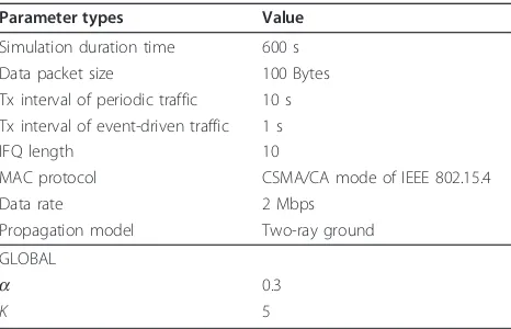
caused by overhearing in GLOBAL is required only in receiving the additional three header fields,hcnt, sum_-redr, andmax_redr(Their total size for the three fields is 5bytes.). In our simulations, a packet overhearing requires GLOBAL and CPL to consume more additional energy in receiving the three fields, as compared to SPR. The initial energy of sensor nodes was set to be 1J. Other simulation parameters are summarized in Table 1.

We define four performance metrics as follows.

•Balance factor (BF): We measure the balance factor of traffic load of sensor nodes. BF is utilized to investigate how well the traffic load is balanced across sensor nodes [21]. LetLi be the traffic load of a sensor node i. BF with the nnumber of nodes is defined as Equation 9. Under the configurations where traffic conditions applied to simulations of each routing protocol are different from each other, measuring their BF values looks unfair. In our simu-lations, we therefore investigated the evolution of BF till the lifetime of a network where SPL is used as its underlying routing protocol. SPL is the routing pro-tocol showing the lowest network lifetime. Since the network lifetime of SPL varies depending on net-work scales, Figures 3 and 4 show different x-axis ranges accordingly.

•Network lifetime: Network lifetime can be defined variously according to a type of applications [22]. In GLOBAL, we define the network lifetime in two ways: (a) the time from network deployment to the instant when one of any sensor nodes dies, denoted byLT1, and (b) the time from network deployment

to the instant when P percentage of sensor nodes

Table 1 Simulation parameters

Parameter types Value

Simulation duration time 600 s Data packet size 100 Bytes Tx interval of periodic traffic 10 s Tx interval of event-driven traffic 1 s

IFQ length 10

MAC protocol CSMA/CA mode of IEEE 802.15.4

Data rate 2 Mbps

Propagation model Two-ray ground

GLOBAL

a 0.3

die, denoted by LT%. In particular, theP values are

varied in our simulations.

• Packet delivery ratio (PDR): PDR is defined as the ratio of the total number of data packets received by sinks to the total number of data packets transmitted by sensor nodes.

•Average end-to-end delay: The end-to-end delay is averaged over all surviving data packets from sensor nodes to sinks.

First, we investigate the impact of bon the perfor-mance of GLOBAL in the following section. We also design a heuristic method to choosebbased on observa-tions from simulation results. We introduce simulation results for each of the above-mentioned metrics, and the analysis of routing control overhead in the protocols is presented in Section IV.C

B The impact ofband a heuristic method to chooseb

As shown in Equation 5,bis tunable.bdetermines the shape of the gradient field, which determines GLOBAL’s routing operations. A largerbvalue enables each sensor node to more favor the least-loaded path, while a smaller

bone makes the path excluding the most overloaded

node more favored. The network traffic is more evenly distributed as the least-loaded path is preferred to use. However, a decrease in network lifetime (LT1) is

unavoid-able since only the cumulative path load is not enough information to identify the path including the most over-loaded node. Therefore, there exists a trade-off between the even distribution of traffic load and network lifetime.

To explore the impact of bon the GLOBAL

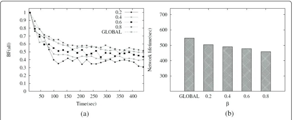
perfor-mance, we evaluated the GLOBAL’s performance with variousbvalues. We measured BF for all sensor nodes (denoted by BF(all)) in the grid scenario whereNis set

to 20. As expected, a largerbvalue makes the BF(all) value for traffic load of sensor nodes to increase, but it makes the network lifetime to decrease as shown in Figure 5. As mentioned in Section III.A.2, settingbto 1 does not make sense, since the gradient value is not guar-anteed to increase with path length.

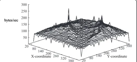
We also captured the load distribution of network traf-fic in the 20x20 grid network with two sinks when SPR was used as a underlying routing protocol. As shown in Figure 6, due to the many-to-one traffic pattern (i.e., con-vergecast traffic to each sink), sensor nodes around sinks tend to be highly overloaded. Since the network lifetime is limited by the lifetime of the most overloaded node among them, the selection of a value should allow traffic to make a detour around the most overloaded node, especially around sinks.

Based on the above observations, we introduce a heuris-tic method to choosebin order to maximize the network

lifetime while minimizing the decrease in BF(all). In GLO-BAL,β= _net−s hcnt_diameter, wheres_hcntis the shortest number of hops to reach a sink from a sensor node (see Algorithm 1) andnet - diameteris the maximum number of hops from one end of the network to the othere_{. Through the} proposed heuristic method, each sensor node is enabled to more favor paths excluding the most overloaded node as its shortest hop distance to a sink decreases. This makes the traffic load of sensor nodes around sinks effectively balanced while allowing sensor nodes far away from sinks to favor the least-loaded path.

Here, for the purpose of demonstrating the effective-ness of the proposed heuristic method, we measured BF (all) and network lifetime (LT1) of GLOBAL under the

same simulation configurations as mentioned above (see Figure 7a). As shown in Figure 7b, GLOBAL shows the best network lifetime with a negligible deterioration in BF(all).

C Performance results

C.1 BF

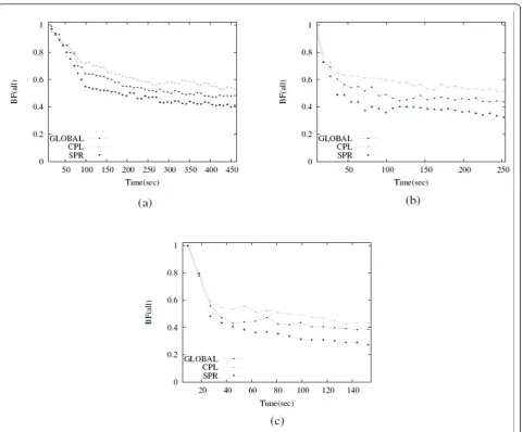
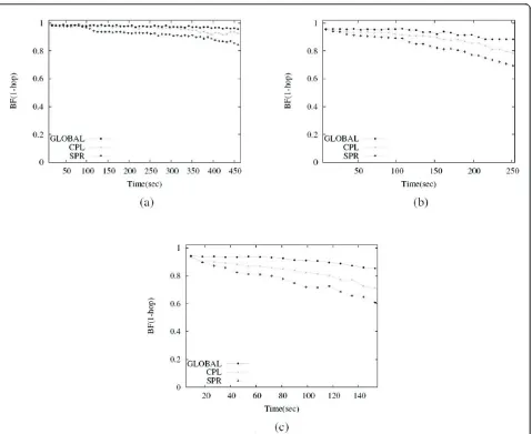
First, for each network scale, we measured the BF(all) value of three compared protocols (GLOBAL, SPR, CPL). Rwas set to 5% in these simulations. Figure 3 shows the evolution of BF(all) for each network scale. At an early stage of the simulation, all the protocols have BF(all) of almost 1 because sensor nodes cannot generate enough traffic to make traffic load distribution unbalanced. For all network scales, similar results are observed.

In a scenario whereNis 20 (see Figure 3a), SPR has a drastic decrease in BF(all) over time, as compared to the other protocols. This is mostly due to the feature of SPR that allows a sensor node to use the same set of links constructing the shortest path in order to forward/relay packets. Eventually, this property heavily loads some nodes and causes them to die earlier. On the other hand, GLOBAL and CPL have better BF(all) than SPR, because both schemes distribute the network traffic through the gradient field constructed based on the cumulative path load of sensor nodes. However, in GLOBAL, since sensor nodes prefer the path excluding the most loaded node to

the least overloaded path as their hop distance to a sink decreases, GLOBAL cannot outperform CPL. GLOBAL outperforms SPR by 3.2%, while CPL outperforms SPR by 12.2% at time 450 s. Table 2 summarizes the perfor-mance gains that GLOBAL and CPL could achieve in terms of BF(all), as compared to SPR. Since the uneven traffic load distribution becomes more serious as the net-work scales, their gains compared to SPR are expected to increase with the network scale.

In order to analyze the impact of increasing a traffic rate on the BF(all) performance, we also measured the BF(all) value of the compared protocols using different Rvalues in the grid scenario where Nwas set to 20. As sensor nodes generate their traffic at a higher rate, sen-sor nodes located in hot spot regions become more overloaded, which makes the distribution of traffic load in the network unbalanced. In this respect, the effect of increasing a traffic rate is almost identical to that of increasing a network scale given a fixed traffic rate. We obtained similar simulation results with each other. Table 3 summarizes the performance gain that GLO-BAL could achieve in terms of BF(all) as compared to the other protocols for different traffic rates.

Due to the characteristics of convergecast traffic to each sink, sensor nodes around sinks tend to be highly overloaded. Since the network lifetime is limited by the lifetime of the most overloaded node among them, it is important to evenly distribute the traffic load around sinks. Based on the reason, we also measured BF for 1-hop neighbor nodes of sinks (denoted by BF(1-1-hop)). In GLOBAL, in order to enable sensor nodes to avoid paths including the most overloaded node, the gradient field is constructed by weighting the cumulative path load as well as the traffic load of the most overloaded node. On the other hand, since CPL creates it gradient field, based

20 ₈₀ 140 ₂₀₀

260 ₃₂₀

380 20 80 140 200

260 320 380 50

100 150 200 250 300

bytes/sec

X-coordinate Y-coordinate bytes/sec

Figure 6Load distribution in the 20 × 20 grid network with two sinks (Coordinates of sinks: (120, 120) and (300, 280)).

on only the cumulative path load, it cannot efficiently avoid using paths containing the most overloaded node. Therefore, CPL produces lower BF(1-hop) than GLO-BAL, as shown in Figure 4. In particular, due to the superiority of GLOBAL’s heuristic method to choose the weighting factor, GLOBAL keeps BF(1-hop) almost close to 1 from 0 to 450 s without significant decrease in BF (all) in case whereNis set to 20 (see Figure 4a). For all network scales, similar results are observed. In this sce-nario, GLOBAL outperforms SPR and CPL by 18.6 and 4.2%, regarding BF(1-hop) at time 450 s, respectively.

Since the uneven traffic load distribution becomes more serious as the network scales, the GLOBAL’s gain in BF is expected to increase with the network scale. Table 4 summarizes the performance gain that GLO-BAL could achieve in terms of BF(1-hop), as compared to the other protocols. In addition, Table 5 summarizes the performance gain that GLOBAL could achieve in terms of BF(1-hop) for differentRvalues in 20 × 20 grid

networks. As mentioned earlier, we observed similar simulation results to those with different network scales. C.2 Network lifetime

Second, we measured the average network lifetime of the compared protocols after running above 50 runs. we define the network lifetime in two ways: LT1and LT%.

Figure 8a showsLT1as a function of network scale. As

mentioned before, sensor nodes around sinks tend to be highly overloaded and the network lifetime is limited by the lifetime of the most overloaded node among them. As shown in Figure 8a, since GLOBAL shows the best BF(1-hop), it also has the bestLT1as expected. In

addi-tion, we observe that the gain inLT1 also increases with

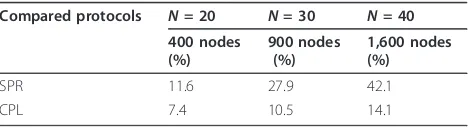
the network scale. Table 6 summarizes the performance

gain that GLOBAL could achieve in terms of LT1 as

compared to the other protocols.

We also measure LT% in 20 × 20 grid networks.

Figure 8b shows how LT% changes by varying the P

Figure 7The performance of GLOBAL: BF(all) and network lifetime.aBF(all).bNetwork lifetime (LT1).

Table 2 The gain of GLOBAL and CPL for different network scales (w.r.t. BF(all))

Protocols N= 20 N= 30 N= 40

400 nodes (%) 900 nodes (%) 1,600 nodes (%)

GLOBAL 8.2 23.4 33.3

CPL 12.2 31.6 45.1

Table 3 The gain of GLOBAL and CPL for different traffic rates (w.r.t. BF(all))

Protocols R= 5 (%) R= 10 (%) R= 15 (%)

GLOBAL 8.2 13.7 18.2

CPL 12.2 21.3 31.2

Table 4 The gain of GLOBAL for different network scales (w.r.t. BF(1-hop))

Compared protocols

N= 20 N= 30 N= 40

400 nodes (%)

900 nodes (%)

1,600 nodes (%)

SPR 18.6 27.9 42.1

CPL 4.2 10.2 20.4

Table 5 The gain of GLOBAL for different traffic rates (w.r.t. BF(1-hop))

Compared protocols R= 5 (%) R= 10 (%) R= 15(%)

SPR 18.6 25.7 30.2

values. Whenever the most overloaded node becomes dead, one of sensor nodes which are still staying alive becomes the most overloaded node newly. Since the GLOBAL’s gradient model reflects the traffic load of the most overloaded node which can be changed over time, GLOBAL efficiently allows sensor nodes to avoid the path including the most overloaded node even after some sensor nodes die. On the other hand, CPL cannot efficiently avoid using paths containing the most over-loaded node. Therefore, GLOBAL keeps its high gain, regardless of the Pvalues as shown in Figure 8b. Table 7 summarizes the performance gain that GLOBAL could achieve in terms ofLT%as compared to the other

protocols. C.3 PDR

Third, we investigated PDR of each protocol. Figure 9 depicts PDR values at the time when the network lifetime is terminated. The unbalance of network traffic load causes a channel around overloaded regions to be con-gested, which leads to the increase in packet loss due to collisions and buffer overflow [12,17]. Hence, since SPR lacks the load-balancing functionality, it shows lower PDR performance than the other load-balancing proto-cols (i.e., GLOBAL, CPL). For example, in case whereN is set to 20, GLOBAL and CPL outperform SPR by 4.5 and 3.3%, respectively. The degree of congestion around overloaded regions become obviously more severe as the

network scales. As expected, both load-balancing proto-cols’gain in PDR increases with the network scale as shown in Figure 9a. For the same reason, the gain of PDR in both load-balancing protocols increases with the traffic rate as shown in Figure 9b. We also examined the causes of packet loss. As shown in Figure 10, most of packet loss results from buffer overflow, followed by packet colli-sions. Since sensor nodes cannot have an abundant sto-rage to buffer packets in resource-constrained WSNs, our simulation set the buffer size to 10 packets.

As observed in previous simulation results, sensor nodes around sinks become highly overloaded and GLOBAL can balance the traffic load, especially around sinks. Therefore, GLOBAL allows more packets to reach sinks than CPL. That is, it shows better PDR than CPL. GLOBAL outper-forms CPL by 3.3% in case whereNis set to 20 and the GLOBAL’s gain in PDR increases with the network scale as shown in Figure 9. Tables 8 and 9 summarize the per-formance gain that GLOBAL could achieve in terms of PDR for different network scales and traffic rates, respectively.

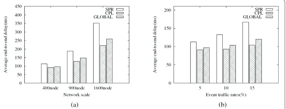
C.4 Average end-to-end delay

Finally, we measured the average end-to-end delay of the compared protocols for different network scales and traffic rates. As shown in Figure 11, the average end-to-end delays of GLOBAL and CPL are lower than those of SRP. This is because both protocols prefer a path with light traffic load and thus reduce the queuing delay in the packet buffer. However, since GLOBAL requires a sensor

Figure 8Performance comparison (w.r.t. Network lifetime).aLT1,bLT%.

Table 6 The gain of GLOBAL (w.r.t.LT1)

Compared protocols N= 20 N= 30 N= 40

400 nodes (%)

900 nodes (%)

1,600 nodes (%)

SPR 11.6 27.9 42.1

CPL 7.4 10.5 14.1

Table 7 The gain of GLOBAL (w.r.t.LT%)

Compared protocols P= 10 (%) P= 20 (%) P= 30 (%)

SPR 15.9 24.1 23.45

node to favor the path excluding the most loaded node as its hop distance to a sink decreases, the traffic load of the selected path may be higher than that of the least-loaded path. Therefore, GLOBAL has a slightly higher average end-to-end delay than CPL, but the difference is negligible. Since the traffic load of the path increases with the amount of traffic generated from the network, the GLO-BAL’s gain is expected to decrease with the network scale and traffic rate, as compared to CPL. Tables 10 and 11 summarize the performance gain that GLOBAL could achieve in terms of the average end-to-end delay for differ-ent network scales and traffic rates, respectively.

C.5 Analysis of routing overhead

Normalized routing load (NRL) is defined as the number of control packets transmitted per data packet delivered at the destination. NRL has been commonly used to evaluate the overhead of routing protocols. In the compared proto-cols, the ADV packet is the only control packet and sinks flood the ADV packet only once when a network is

initialized. Therefore, they have almost the same NRL among each other. Unlike SPR, GLOBAL and CPL, how-ever, require sensor nodes to piggyback control informa-tion on the periodic data packet. We therefore measured their byte-level control overhead, since NRL cannot reflect the control overhead caused by the piggybacking. In the compared protocols, the overhead is affected by three parameters: the size of information piggybacked on the periodic data packet, the period of the periodic data trans-mission, and the number of sensor nodes. Since we have fixed values for such parameters, their byte-level control over-head was measured numerically without simulations.

In GLOBAL, sensor nodes are allowed to piggyback the 5-byte information (i.e.,hcnt,sum_redr, andmax_redr) on their periodic data packet. On the other hand, CPL requires the 3-byte information (i.e.,hcntandsum_redr) to be piggybacked on the periodic data packet, and SPR does not require any piggybacking. Therefore, assuming that there areNsensorsensor nodes and they transmitk

periodic data packets per second, GLOBAL and CPL have the routing overhead of 5 ·Nsensor·k bytes/sand 3 ·Nsensor

·kbytes/s, respectively. In addition, the routing overhead caused by the ADV flooding is calculated to beLADV ·

Nsink·Nsensorbytes, whereLADVis the length of the ADV

message in bytes andNsinkis the number of sinks.

V Conclusion

For the purpose of load balancing, the cumulative traffic load of a path is considered in existing gradient routing protocols. However, they have a critical drawback that a sensor node cannot efficiently avoid using the path with the most overloaded node. Only the information on cumulative path load is not enough to identify the path including the most overloaded node. Hence, we proposed a new gradient routing protocol (called GLOBAL). In

Figure 9Performance comparison (w.r.t. PDR).aPDR for different network scales,bPDR for different traffic rates.

GLOBAL, each sensor node determines its gradient by weighting the cumulative load of a path and the most overloaded node over the path through a weight factorb. Using ns-2 simulator, we explored the impact ofbon the GLOBAL performance and found that there exists a trade-off between the even distribution of traffic load and network lifetime. Based on simulation results, we intro-duced a heuristic method to choosebin order to maxi-mize network lifetime while minimizing deterioration in load-balancing performance. Through the proposed heuristic method, each sensor node is enabled to more favor paths excluding the most overloaded node as its shortest hop distance to a sink decreases. This makes the traffic load of sensor nodes around sinks effectively balanced while allowing sensor nodes far away from sinks to favor the least-loaded path. In addition, we also pro-posed an addressing-free forwarding strategy in order to avoid addressing overhead. Instead of using an address

for forwarding packets, GLOBAL uses the gradient value as the next-hop node identifier.

Through ns-2 simulation, we conducted performance comparisons with other routing protocols in static grid networks: shortest path routing (SPR) and CPL, where CPL is a gradient routing using the cumulative path load only. We measured four metrics: balance factor, network lifetime, packet delivery ratio, and average end-to-end delay. GLOBAL always achieves better perfor-mances than the others in terms of the former three metrics. In particular, assuming that the network life-time is defined as the life-time from network deployment to the instant when one of any sensor nodes dies, GLO-BAL shows the performance improvements in the net-work lifetime by 42.1 and 14.1% at a 40 × 40 grid network, as compared to SPR and CPL, respectively. This implies that GLOBAL can achieve its main goal of extending the network lifetime. However, GLOBAL has a slightly higher average end-to-end delay than CPL, but the difference is negligible. In this work, GLOBAL did not take the mobility of sensor nodes and sinks into account. Its performance degradation in dynamic net-works with node mobility is unavoidable. Hence, its robustness against the frequent change of network topology will be improved in our future work.

Endnotes

a_{The cumulative traffic load information of the path is}

simply called as cumulative path load.

b_{A simple battery life indicator based solely on the}

battery voltage cannot provide high-resolution measure-ment. Resolution refers to the smallest quantity of energy that a system can measure. However, more sophisticated devices can measure their battery level

Table 8 The gain of GLOBAL for different network scales (w.r.t. PDR)

Compared protocols

N= 20 N= 30 N= 40

400 nodes (%)

900 nodes (%)

1,600 nodes (%)

SPR 4.5 13.65 23.6

CPL 3.3 6.45 13.3

Table 9 The gain of GLOBAL for different traffic rates (w. r.t. PDR)

Compared protocols R= 5 (%) R= 10 (%) R= 15 (%)

SPR 4.5 5.18 8.4

CPL 3.3 4.1 5.3

based on the average of the energy drained from the battery. As mentioned in [19], high-resolution battery measuring can be performed using either hardware sup-port, as in systems like Quanto [23] and iCount [24], or using software monitoring, as in Pixie [25] and a resolu-tion of 0.1μJ can be achieved.

c_{Ye et al. [4] proposed an efficient backoff-based}

gra-dient field establishment algorithm, which attempts to find the optimal costs of all nodes to the sink with the overhead of one packet per node. Although GLOBAL currently utilizes the naive flooding-based gradient field establishment algorithm, it can simply adopt the back-off-based one. The performance improvement issue in the gradient field establishment algorithm is out of scope of this paper.

d_{Assuming that sinks and sensor nodes have no}

mobi-lity, the evaluation of performance in dynamic networks is beyond the scope of this work.

e_{net - diameter is a system parameter. The}

calcula-tion ofnet - diameteris out of scope of this paper.

Author details

1_{Graduate School of Electrical Engineering and Computer Science,}

Kyungpook National University, Daegu, Korea2_{School of Computer Science}

and Engineering, College of IT Engineering, Kyungpook National University, Daegu, Korea

Competing interests

The authors declare that they have no competing interests.

Received: 15 June 2010 Accepted: 1 September 2011 Published: 1 September 2011

References

1. M Perillo, Z Cheng, W Heinzelman, Strategies for Mitigating the Sensor Network Hot Spot Problem, inProceedings of MobiQuitous(July 2005) 2. D Puccinelli, M Haenggi, Arbutus: Network-Layer Load Balancing for

Wireless Sensor Networks, inProceedings of IEEE WCNC(April 2008) 3. I Slama, B Jouaber, D Zeghlache, Energy Efficient Scheme for Large Scale

Wireless Sensor Networks with Multiple Sinks, inProceedings of IEEE WCNC

(March 2008)

4. F Ye, A Chen, S Lu, L Zhang, A Saclable Solution to Minimum Cost Forwarding in Large Sensor Networlks, inProceedings of IEEE ICCCN

(October 2001)

5. JN Al-Karaki, AE Kamal, Routing techniques in wireless sensor networks: a survey. IEEE Wirel Commun.11(6), 6–28 (2004). doi:10.1109/

MWC.2004.1368893

6. P Huang, H Chen, G Xing, Y Tan, SGF: a state-free gradient-based forwarding protocol for wireless sensor networks. ACM Trans Sen Netw. 5(2), 1–25 (2009)

7. A Basu, A Lin, S Ramanathan, Routing Using Potentials: A Dynamic Traffic-Aware Routing Algorithm, inProceedings of ACM SIGCOMM(August 2003) 8. RH Cheng, SY Peng, C Huang, A Gradient-Based Dtnamic Load Balance

Data Forwarding Method for Multi-Sink Wireless Snesor Networks, in

Proceedings of IEEE APSCC(December 2008)

9. H Liu, ZL Zhang, J Srivastava, V Firoiu, PWave: A Multi-Source Multi-Sink Anycast Routing Framework for Wireless Sensor Networks, inProceedings of IFIP Networking(May 2007)

10. RC Shah, JM Rabaey, Energy Aware Routing for Low Energy Ad Hoc Sensor Networks, inProceedings of IEEE WCNC(March 2002)

11. J Suhonen, M kuorilehto, M Hannikainen, TD Hamalainen, Cost-Aware Dynamic Routing Protocol for Wireless Sensor Networks–Design and Prototype Experiments, inProceedings of IEEE PIMRC(September 2006) 12. M Fyffe, M Sun, X Ma, Traffic-Adapted Load Balancing in Sensor Networks

Employing Geographic Routing, inProceedings of IEEE WCNC(March 2006) 13. S Singh, M Woo, CS Raghavendra, Power-Aware Routing in Mobile Ad Hoc

Networks, inProceedings of ACM/IEEE MobiCom(October 1998)

14. R Draves, J Padhye, B Zill, Routing in Multi-Radio, Multi-Hop Wireless Mesh Networks, inProceedings of ACM/IEEE MobiCom(September 2004) 15. F Ye, G Zhoung, S Lu, L Zhang, GRAdient broadcast: a robust data delivery

protocol for large scale sensor networks. Wirel Netw.11(3), 285–298 (2005). doi:10.1007/s11276-005-6612-9

16. T Roosta, WC Liao, WC Teng, S Sastry, Testbed Implementation of a Secure Flooding Time Synchronization Protocol, inProceedings of IEEE WCNC

(March 2008)

17. K Wu, J Harms, Load-Sensitive Routing for Mobile Ad Hoc Networks, in

Proceedings of IEEE ICCCN(October 2001)

18. D Kim, JJ Garcia-Luna-Aceves, K Obraczka, J-C Cano, P Manzoni, Routing mechanisms for mobile ad hoc networks based on the energy drain rate. IEEE Trans Mob Comput.2(2), 161–173 (2003). doi:10.1109/

TMC.2003.1217236

19. GW Challen, J Waterman, M Welsh, Idea: Integrated Distributed Energy Awareness for Wireless Sensor Networks, inProceedings of ACM MobiSys

(June 2010)

20. P Basu, J Redi, Effect of Overhearing Transmissions on Energy Efficiency in Dense Sensor Networks, inProceedings of IEEE IPSN(April 2004)

21. H Dai, R Han, A Node-Centric Load Balancing Algorithm for Wireless Sensor Networks, inProceedings of IEEE GLOBECOM(December 2003)

22. Y Chen, Q Zhao, On the lifetime of wireless sensor networks. IEEE Commun Lett.9, 976–978 (2005). doi:10.1109/LCOMM.2005.11010

23. R Fonseca, P Dutta, P Levis, I Stoica, Quanto: Tracking Energy in Networked Embedded Systems, inProceedings of OSDI(December 2008)

24. P Dutta, M Feldmeier, J Paradiso, D culler, Energy Metering for Free: Augmenting Switching Regulators for Real-Time Monitoring, inProceedings of IEEE IPSN(April 2008)

25. K Lorincz, B Chen, J Waterman, G Werner-Allen, M Welsh, Resource Aware Programming in the Pixie os, inProceedings of ACM SenSys(November 2008)

doi:10.1186/1687-1499-2011-85

Cite this article as:Yooet al.:A scalable multi-sink gradient-based

routing protocol for traffic load balancing.EURASIP Journal on Wireless

Communications and Networking20112011:85.

Table 10 The gain of GLOBAL for different network scales (w.r.t. Average end-to-end delay)

Compared

Table 11 The gain of GLOBAL for different traffic rates (w.r.t. Average end-to-end delay)

Compared protocols R= 5 (%) R= 10 (%) R= 15 (%)

SPR 14.2 21.85 28.4