© 2017 The Authors. Published by Innovare Academic Sciences Pvt Ltd. This is an open access article under the CC BY license (http://creativecommons. org/licenses/by/4. 0/) DOI: http://dx.doi.org/10.22159/ajpcr.2017.v10s1.20767
Advances in Smart Computing and Bioinformatics
DETECTION OF WHALES USING DEEP LEARNING METHODS AND NEURAL NETWORKS
SAHEB GHOSH*, SATHIS KUMAR B, KATHIR DEIVANAI
Department of Computer Science, VIT University, Chennai, Tamil Nadu, India. Email: [email protected] Received: 23 January 2017, Revised and Accepted: 03 March 2017
ABSTRACT
Deep learning methods are a great machine learning technique which is mostly used in artificial neural networks for pattern recognition. This project is to identify the Whales from under water Bioacoustics network using an efficient algorithm and data model, so that location of the whales can be send to the Ships travelling in the same region in order to avoid collision with the whale or disturbing their natural habitat as much as possible. This paper shows application of unsupervised machine learning techniques with help of deep belief network and manual feature extraction model for better results.
Keywords: Deep learning, Whale detection, Neural network, Machine learning.
INTRODUCTION
Detection of underwater creatures is not an explored area of science until now. So looking back, we found only few people who have tried to apply machine learning for detection or classification of marine animals. Cornell university whale detection program [1, 2, 3, 4, 5] provides extensive information about whale detection a and its importance The data used here is taken from Kaggle competition[6] of whale detection, sponsored by Cornell university. Mellinger and Clark [1] looked at a few techniques for perceiving bowhead whale calls. They proposed a system utilizing spectrogram relationship and contrasted this with three other systems, which utilized a hidden Markov model (HMM), a coordinated channel and a neural system, individually. The HMM system is similar to the one utilized by Weisburn et al. The data layer of the neural system was a [11,22] exhibit processed from the spectrogram. The shrouded layer contained four units, what’s more, the yield layer contained a solitary unit. Each of the system gave back a score which were contrasted with an edge for figuring out if a call was distinguished. The main data set was utilized for contrasting the spectrogram connection system with the strategy utilizing a HMM and the strategy utilizing a coordinated channel while the second Data set was utilized for looking at the spectrogram relationship system to the strategy utilizing a neural system and the technique utilizing a coordinated channel. Mellinger and Clark found that, the spectrogram relationship system performed imperceptibly superior to the technique utilizing a HMM, and that the system utilizing a neural system performed far better. In any case they additionally found that the neural system requires a moderately expansive data set for learning. Further they found that the match channel performed inadequately, and they inferred that the coordinated channel strategy is not suitable in light of the fact that the problem in the recordings were not Gaussian [12] disseminated, and the bowhead whale calls were excessively disparate from each other. RELATED WORK
The objective of perceiving marine creature sounds has been implemented by a few people in the past utilizing different techniques:
Brown and Smaragdis [11] ordered calls from executioner whales into seven distinctive call sorts. They explored the utilization of Gaussian mixture models (GMMs) and HMMs [25] where the HMMs had a GMM for every state. Their data comprised of 75 recorded calls which each contained one and one and only of the seven call sorts. As highlight information the mel-frequency cepstral coefficients (MFCCs) [27] and their transient subsidiaries were utilized. These
were ascertained utilizing the project MELCPST from the Matlab [8] perceiving marine creature sounds is an issue that has incredible closeness to discourse acknowledgment.
Data and Sturtivant [13] utilized HMMs to distinguish three distinct gatherings of dolphin shrieks. Their HMMs spoke to the form of the state of the dolphin shriek when drawn as a spectrogram. For each of their sound recordings, the part that contained a dolphin shriek was recognized in the preprocessing, and a spectrogram representation of this was developed. At that point from taking after calculation was connected on the spectrogram to discover the state of shriek sound. A HMM was educated for every shriek class. These were then utilized for characterizing future shrieks by figuring the probability that a recorded shriek has a place with every class.
Roch et al. [29] utilized GMMs to decide the types of recorded dolphin shrieks. The recorded sign was part up into time allotments from
which the cepstral coefficients were computed. These were then
utilized as highlight information for the GMMs. A GMM was gained from the shrieks for each species. At the point when the species for a recorded shriek was resolved, the probability for each GMM speaking to the component information was ascertained. The dolphin that made the shriek was then expected to have a place with the animal categories whose GMM had given back the most elevated probability. The number of segments of the GMMs was 64, 128, 256, and 512. The best results were discovered utilizing GMMs with 256 blends. Weisburn et al. [34] researched two distinct routines for recognizing
bowhead whale brings in sound recordings which were recorded in the arctic. Other than bowhead calls they contained commotion, and, potentially impedances made by different creatures, or by ice that was breaking. The two distinct routines, that they utilized, were a HMM and a coordinated channel. The component information for the HMM was the three biggest crests in the recurrence range for every time period. The Gee had 18 states, and for each of these it had a Gaussian conveyance [28] over the component information. The coordinated channel was resolved from 40 recordings that contained just whale calls and no impedances. These recordings were likewise used to take in the HMM. Keeping in mind the end goal to recognize whale calls in the recorded signs, they figured a score and contrasted it with an edge. For the HMM the score was the probability found by the Viterbi calculation, and for the coordinated channel it was the connection between the sign and the channel. Weisburn et al. found that their HMM technique performed superior to the technique utilizing a coordinated channel, however both strategies distinguished a high partition wrongly.
For both issues we are attempting to characterize sound signs by the source which produced them. Therefore it is the specific source, that we are attempting to perceive, which recognizes the issues. For discourse acknowledgment we realize that the source is a human vocal tract, and we are attempting to perceive the setting of this vocal tract. For the issue tended to by this venture, the source could have been a right whale which radiated an up-call. Else it could likewise some other source e.g., other marine creatures. For both issues we must concentrate highlight information which convey data about the procedure that produced the sign, and from this learn models which catch the procedure that produced the sign. Discourse acknowledgment is an issue that has been widely examined in the past [24,26,30], and due to its comparability to our issue it is sensible to research how techniques for discourse acknowledgment can be connected to perceiving up calls. Roch et al. [29] and Brown and Smaragdis [11] utilized a methodology exceptionally like the one that was proposed for discourse acknowledgment by Rabiner in 1989 [26]. They too utilized the Cepstral coefficients which are utilized frequently as a part of discourse acknowledgment on the grounds that it conveys much data about the vocal tract [23] tool kit Voicebox [7]. Testing was performed utilizing the forget one technique where each recording from the data set thusly was grouped while the remaining were utilized for learning the models. To quantify execution the rate understanding was utilized. The GMMs [9,10] were learned with 1-6 segments and 8-30 highlights. The best result was 92% understanding which was acquired utilizing GMMs with two segments and 30 highlights. The HMMs was scholarly with 5-17 states, 1-4 parts, and 8-42 highlights. The best results were 95% ascension, which was acquired utilizing HMMs with 24-30 highlights, 13-17 states, and one segment.
APPROACH
All the methods mentioned above follows a feature extraction by a manual process. However, after invention of deep learning techniques in machine learning it is possible to ask the machine to identify patterns and feature with proper training. Neural systems are effective example classifiers which have been utilized as a part of various order and capacity guess undertakings. They are exceedingly nonlinear classifiers not just since they have nonlinear actuation units additionally in light of the fact that of the layer-wise structure stacked in a steady progression. Such a structure empowers the neural networks (NNs) to take in the mind boggling info yield connections of numerous grouping issues, for example, acoustic occasion grouping.
Our main focus here is to extract as many features as possible. The major disadvantage of analyzing audio files is that they contain lots of noise. Therefore a more prudent approach is to convert the audio files to Fig. files i.e., fast Fourier transformation, then use sliding window method to extract multiple features. Manufactured neural systems are prepared in a regulated way with the back propagation calculation in which the arbitrarily instated system weights are balanced concurring to the inclination plunge standard to take in the info yield relations from marked information. Back propagation calculation performs viably for shallow systems, i.e. those that have 1 or 2 concealed layers, yet its execution decays when the number of layers increments. Various investigations appear that the calculation gets stuck in neighborhood optima effortlessly and falls flat to sum up legitimately for profound systems [13,14] (with a conceivable exemption of convolutional neural systems, which were observed to be less demanding to prepare notwithstanding for more profound architectures [15,16]). All in all, it is demonstrated that, when NN weights are arbitrarily instated, profound neural systems perform more regrettable than the shallow ones [13,17]. With a specific end goal to facilitate the preparation of profound systems, an unsupervised pre-preparing is directed layer by layer, to instate the system weights [18]. This insatiable, layer-wise unsupervised pre-training depends on confined boltzmann machine (RBM) generative model. A calculation called contrastive dissimilarity (album) is connected to prepare a RBM. Compact disc calculation prepares the
first layer in an unsupervised way, delivering a starting arrangement of coefficients for the first layer of a NN. At that point, the yield of the main layer is bolstered as information to the following, again introducing the relating layer in an unsupervised way. The scientific points of interest of the CD calculation, can be found in [19] and won’t be introduced in this work. In the wake of pre-training, neural systems are prepared in a directed way with group back propagation calculation in which the weight overhauls happen after various preparing tests is exhibited to the system (group size). This stride serves as an adjusting procedure of the neural system coefficients [20] that have gone with pre-training. In this work, the topology of the neural system (5 covered up layers each containing 70 neural units with sigmoid actuation capacities) is picked by approval set and the impact of varieties in system topology on the characterization exactness is not displayed. Preparing parameters for the neural systems, for example, learning rate, energy, bunch size and so forth as well as their topology are kept the same for the majority of the investigations. The bunch size for both unsupervised and directed parts is decided to be 100. The learning rate and force of back propagation [21] are chosen to be 0.5 and 1 individually. The number of ages for the unsupervised pre-training is altered to two. The basis for ceasing the directed preparing was in light of the approval set mistake. The preparation was ended at the point when the acceptance mistake began to build which is a sign of over fitting [35].
MODULES
There are three different modules:
A. The features extraction module, which will read the dataset and extract features based on deep NN. The extraction is done in two
parts first using deep learning techniques and second extracting few
features with help of Numpy and Sklearn python library functions. B. Data analyzing and modeling module.
C. Re-evaluation and back propagation module (Fig. 1). FEATURES USED
High frequency template
Apply horizontal contrast enhancement and look for strong vertical features in the Fig. cut out the lower frequencies.
Fig. 1: Complete architecture of the proposed model
a
b
High frequency metrics
Calculate statistics of features at higher frequencies [31] This is designed to capture false alarms that occur at frequencies higher than typical whale calls.
Also sum across the frequencies to get an average temporal profile. Then return statistics of this profile. The false alarms have a sharper peak.
Time metrics
Calculate statistics for a range of frequency [32] slices.
Calculate centroid, width, skew, and total variation [33]. let x=P[i,:], and t=time bins
centroid=sum(x*t)/sum(x)
width=sqrt(sum(x*(t-centroid)^2)/sum(x)) skew=scipy.stats.skew
total variation=sum(abs(x_i+1-x_i)).
All these three types of features are at first filtered against Sliding Window and various frequency or X, Y coordinate.
IDENTIFIED TOOLS
MatlabR2014, Python 3.4 both of these required for Reading the audio files and extracting the features. The data model can be built in any of these two. We have also used Sklearn and Numpy libraries for statistical calculations.
b a
Fig. 3: Three dimensional spectrogram of a audio containing whale sound
Fig. 4: Spectrogram of sound without whale voice
Fig. 6: Fast Fourier transform of a sound which does not contain whale voice
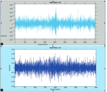
Fig. 7: Sample with whale call (cropped)
Fig. 9: Frequency distribution without a whale call
Fig. 10: Receiver operating characteristic curve
Rank Extracted feature Importance
1 maxH_0005501 0.0373
2 maxH_0001315 0.033032
3 maxH_0000151 0.021753
4 maxH_0003507 0.020955
5 max_0000151 0.019671
6 maxH_0006245 0.018837
7 max_0004355 0.017471
8 max_0001315 0.016203
9 maxH_0001347 0.015726
10 skewTime_0027 0.01521
11 bwTime_0001 0.014406
12 maxH_0006722 0.013614
13 maxH_0002307 0.012322
14 bwTime_0006 0.011176
15 max_0001347 0.011116
16 max_0005501 0.010813
17 yLocH_0004631 0.010806
18 max_0003507 0.010696
19 max_0006340 0.0106
20 maxH_0005360 0.010428
21 skewTime_0050 0.010049
22 centOops_0002 0.009445
23 max_0006245 0.009411
24 centOops_0006 0.00888
25 bwTime_0002 0.00886
26 bwTime_0034 0.008708
Rank Extracted feature Importance
27 skewTime_0031 0.008067
28 yLoc_0001315 0.00794
29 maxH_0004355 0.007474
30 maxH_0001236 0.007401
31 tvTime_0005 0.007322
32 bwTime_0000 0.007204
33 bwTime_0048 0.006806
34 max_0001236 0.006698
35 skewTime_0023 0.005678
36 tvTime_0000 0.005587
37 skewTime_0042 0.005575
38 skewTime_0011 0.005341
39 bwTime_0012 0.005291
40 maxH_0001312 0.005287
41 skewTime_0044 0.005073
42 yLoc_0000151 0.004998
43 skewTime_0022 0.004918
44 tvTime_0009 0.004874
45 max_0006722 0.004849
46 skewTime_0032 0.004485
47 bwTime_0049 0.00443
48 skewTime_0012 0.004246
49 centTime_0004 0.004014
50 bwTime_0037 0.004001
51 centOops_0005 0.003918
52 tvTime_0052 0.003822
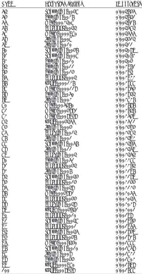
Table 1: Top features based on execution Table 1: (Continued)
(Contd...) (Contd...)
Fig. 8: (a and b) Whale component frequency filter b
RESULTS AND SCREENSHOTS
The frequency based filter on whale component analysis shows us the major difference between a sample containing whale voice and a sample not containing whale voice (Figs. 6-9). These initial analyses using fast fourier transform (FFT) made us understand the attributes of whale voices. Therefore, we decided to work on manual feature extraction based on frequency. The extracted features of high frequency template, high frequency metrics and time metrics has been sorted in order of importance towards the result accuracy in Table 1.
The receiver operating characteristic (ROC) analysis shows that we have achieved (AUC) area under curve of 0.9857831 analysis for our approach (Fig. 10).
CONCLUSION
The current work shows an efficient feature based highly accurate method of detection of whale voices from underwater captured audio files with more than 97% accuracy.
Rank Extracted feature Importance
Table 1: (Continued) FUTURE WORK
In near future the similar approach can be used for other applications as well like, detection of audio from deep space observations for intelligent species search, even it can be used in other image or audio detection problems. The current model works very well with audio files with less noise. Another improvement can be done on detection of required signal on noisy files.
1. Cornell University’s Bioacoustics Research Program. Available from: http://www.birds.cornell.edu/brp. [Last retrieved on 2013 Apr 29]. 2. Kaggle. Available from: https://www.kaggle.com. [Last retrieved on
2013 Apr 22].
3. The Marinexplore and Cornell University Whale Detection Challenge. Available from: https://www.kaggle.com/c/whale-detection-challenge. [Last retrieved on 2013 Apr 22].
4. The Marinexplore and Cornell University Whale Detection Challenge Forum. Available from: http://www.kaggle.com/c/whale-detection-challenge/forums. [Last retrieved on 2013 Apr 22].
5. Right Whale Listening Network. Available from: http://www. listenforwhales.org. [Last retrieved on 2013 Apr 29].
6. Marinexplore. Available from: http://www.marinexplore.org. [Last retrieved on 2013 Apr 29].
7. Voicebox: Speech Processing Toolbox for MatLab. Available from: http://www.ee.ic.ac.uk/hp/staff/dmb/voicebox/voicebox.html. [Last retrieved on 2013 Apr 22].
8. Compute Receiver Operating Characteristic (ROC) Curve or other Performance Curve for Classifier Output. Available from: http:// www.mathworks.se/help/stats/perfcurve.html. [Last retrieved on 2013 May 23].
9. Is a Sample Covariance Matrix Always Symmetric and Positive Definite? Available from: http://www.stats.stackexchange.com/ questions/52976/is-a-sample-covariance-matrix-always-symmetric-and-positive-definite. [Last retrieved on 2013 Apr 30].
10. Bilmes JA. A gentle tutorial of the EM algorithm and its application to parameter estimation for Gaussian mixture and hidden Markov models. Intern Comput Sci Inst 1998;4(510):126.
11. Brown JC, Smaragdis P. Hidden Markov and Gaussian mixture models for automatic call classification. J Acoust Soc Am 2009;125(6):EL221-4. 12. Cormen TH, Leiserson CE, Rivest RL, Stein C. Introduction to
Algorithms. 2nd ed. Cambridge, MA, USA: The MIT Press; 2001. 13. Rumelhart DE, Hinton GE, Williams RJ. Learning Representations by
Back-Propagating Errors. Cambridge, MA, USA: MIT Press; 1988. 14. Hinton GE, Salakhutdinov RR. Reducing the dimensionality of data
with neural networks. Science 2006;313(5786):504-7.
15. Lee H, Grosse R, Ranganath R, Ng AY. Convolutional deep belief networks for scalable unsupervised learning of hierarchical representations. In: Proceedings of the 26th Annual International Conference on Machine Learning. ACM; 2009. p. 609-16.
16. Simard P, Steinkraus D, Platt JC. Best practices for convolutional neural networks applied to visual document analysis. ICDAR 2003;3:958-62. 17. Erhan D, Manzagol PA, Bengio Y, Bengio S, Vincent P. The difficulty of
training deep architectures and the effect of unsupervised pre-training. In: International Conference on Artificial Intelligence and Statistics; 2009. p. 153-60.
18. Hinton GE, Osindero S, Teh YW. A fast learning algorithm for deep belief nets. Neural Comput 2006;18(7):1527-54.
19. Bengio Y. Foundations and trends in machine learning. Learning Deep Architectures for AI. Vol. 2. Hanover, MA: Now Publishers Inc.; 2009. p. 1-127.
20. Leon SJ. Linear Algebra with Applications. Maxwell Macmillan International Edition. New York: Pearson; 2006.
21. McAllester D. The Covariance Matrix. Course TTIC 103 (CMSC 35420): Statistical Methods for Artificial Intelligence, at Toyota Technological Institute at Chicago, Autumn; 2007. Available from: http://www.ttic.uchicago.edu/~dmcallester/ttic101-07/lectures/ Gaussians/Gaussians.pdf. [Last retrieved on 2013 Apr 14].
22. Mellinger DK, Clark CW. Recognizing transient low-frequency whale sounds by spectrogram correlation. J Acoust Soc Am 2000;107:3518-29.
24. Owens FJ. Signal processing of speech. Macmillan New Electronics Series. McGraw-Hill Ryerson, Limited; 1993. Available from: http:// www.books.google.dk/books?id=qpAeAQAAIAAJ.
25. Rabiner L, Juang BH. Fundamentals of Speech Recognition. Englewood Cliffs: Prentice Hall; 1993.
26. Rabiner LR. A tutorial on hidden Markov models and selected applications in speech recognition. In: Proceedings of the IEEE; 1989. p. 257-86.
27. Reby D, Andre-Obrecht R, Galinier A, Farinas J, Cargnelutti B. Cepstral coefficients and hidden markov models reveal idiosyncratic voice characteristics in red deer (Cervus elaphus) stags. J Acoust Soc Am 2006;120(6):4080-9. Available from: http://www.sro.sussex.ac.uk/756. 28. Douglas Reynolds. Gaussian mixture models. Encyclopedia of
Biometric Recognition. Amsterdam, Netherlands: Springer; 2008. p. 14-68.
29. Roch MA, Soldevilla MS, Burtenshaw JC, Henderson EE, Hildebrand JA. Gaussian mixture model classification of odontocetes in the Southern California bight and the Gulf of California. J Acoust Soc Am 2007;121(3):1737-48. Available from: http://www.
biomedsearch.com/nih/Gaussian-mixture-model-classification-odontocetes/17407910.html.
30. Russell SJ, Norvig P, Canny JF, Malik JM, Edwards DD. Artificial Intelligence: A Modern Approach. 2nd ed. Englewood Cliffs: Prentice Hall; 1995.
31. Spaulding E, Robbins M, Calupca T, Clark CW, Tremblay C, Waack A, et al. An autonomous, near-real-time buoy system for automatic detection of north Atlantic right whale calls. Proc Meet Acoust 2009;6(1). DOI: 10.1121/1.3340128. Available from: http://www.link. aip.org/link/?PMA/6/010001/1.
32. Tan PN, Steinbach M, Kumar V. Introduction to Data Mining. 1st ed. Boston, MA, USA: Addison-Wesley Longman Publishing Co., Inc.; 2005.
33. Vaseghi SV. Advanced Digital Signal Processing and Noise Reduction. Wiley; 2008. Available from: http://www.books.google.ca/ books?id=vVgLv0ed3cgC.
34. Weisburn BA, Mitchell SG, Clark CW, Parks TW. Isolating biological acoustic transient signals. In: Acoustics, Speech, and Signal Processing; 1993. ICASSP-93., 1993 IEEE International IEEE; 1993. p. 269-72. 35. Wu CF. On the convergence properties of the EM algorithm. Ann Stat