Deadlock Analysis of Message-Passing Programs with Identical Processes

(1)

JUN ZHOU. Deadlock Analysis of Message-Passing Programs with Identical Processes. (Under the direction of Professor K. C. Tai.)

Deadlocks are a common type of faults in message-passing programs. One approach to detecting deadlocks in a message-passing program is to perform reachability analysis, which involves deriving possible global states of the program. The resulting state graph is referred to as a reachability graph (RG). The size of the RG of a message-passing program, in the worst case, is an exponential function of the number of processes in the program. This problem, referred to as the state explosion problem, makes reachability analysis impractical for message-passing programs with many processes.

Assume that P is a message-passing program that contains one process type T with a dynamic number of instances. Let Pm denote the version of P that has m instances of T. To detect deadlocks in P, we apply reachability analysis to P1, P2, ..., and Pn, where n is an integer chosen randomly or according to some criterion. If the value of n is large, reachability analysis ofPnis impractical. If the value ofnis small, we have little confidence on whether Pk is deadlock-free for any k > n. A deadlock cutoff number c for P means that under certain conditions, if Pc has no deadlocks, then Pk has no deadlocks for any k > c. For message-passing programs that contain two or more process types with dynamic numbers of instances, their deadlock cutoff vectors are defined in a similar way.

(2)

major problem with this approach is that it fails to find deadlock cutoff numbers for many message-passing programs.

To improve the above approach, we define a new equivalence relation called projection equivalence, which is weaker than observational equivalence. The projection of L in Pm, i >0, is defined to be the behavior ofLinPm. The environments ofLinPi andPj,i6=j, are said to be projection equivalent ifLhas the same projection inPi andPj. We show how to apply projection equivalence to find deadlock cutoff numbers for client/server programs and ring-structured programs.

A client/server program contains a server and a number of clients. Clients call the server to request service; they do not communication with each other. The server cannot call individual clients. For client/server programs, we define a new type of reduced reachability graphs, called client/server reachability graphs or CSRGs. The size of the CSRG of a client/server program is a polynomial function of the number of clients. Based on CSRGs, we show how to determine the existence of a deadlock cutoff number for a client/server program and how to find this number if it exists. We also show how to find deadlock cutoff vectors for client/server programs with two or more types of clients.

(3)

Identical Processes

by

Jun Zhou

A thesis submitted to the Graduate Faculty of North Carolina State University

in partial fulfillment of the requirements for the Degree of

Doctor of Philosophy

Department of Computer Science

Raleigh 2000

APPROVED BY:

(4)

To my wife

Yanyu Liu,

(5)

BIOGRAPHY

(6)

ACKNOWLEDGEMENTS

I would like to thank my advisor, Dr. K. C. Tai, for his guidance. His intuition and enthusiasm have been very inspiring. I sincerely thank Dr. Harry Perros, Dr. Mladen A. Vouk, and Dr. S. Purush Iyer who kindly accept my invitation to be on my advisory committee.

I thank my wife for her love and support.

(7)

List of Figures

2.1 Illustration of LTS systems . . . 7

2.2 (a) ring-structured LTS system P8 and (b) ring-plus-structured LTS system P7 . . . 9

2.3 Recursive model checking algorithm forP: EF(“T=1”) . . . 12

2.4 Recursive model checking algorithm forQ: EG(“T=1”) . . . 13

2.5 Illustration of deadlocks . . . 15

4.1 Ring-structured LTS systemP6 . . . 23

4.2 Ring-plus-structured LTS system Pm . . . 25

4.3 Env₍_m,i₎ in ring-plus-structured LTS systems . . . 26

4.4 Solution two for the DP problem . . . 31

5.1 Illustration of projection operation. . . 36

5.2 An counter example . . . 40

5.3 Illustration of Theorem 5.2.2 . . . 44

5.4 Illustration of Theorem 5.3.1 with k=3, m=1 . . . 49

5.5 An application of algorithms Find DCN 5.3 and Find DCN 5.3 Refine . . . 53

5.6 Illustration of Theorem 5.4.1 with m=1 . . . 55

6.1 From RG toCSRG . . . 65

6.2 Illustration of Algorithm Extend() . . . 69

6.3 Illustration of Theorem 6.1.1 . . . 70

6.4 Find a deadlock cutoff number using CSRGs . . . 74

6.5 An example to illustrate that the server allows unbounded number of clients to be active. . . 76

6.6 Illustration of a deadlock cutoff vector . . . 83

6.7 The LTS specification for CSMA/CD . . . 91

6.8 LTSs for tasksRW3,Reader,W riter and (Reader||W riter) . . . 93

7.1 An example client/server ECFSM program . . . 105

7.2 The operator in Solution 3 . . . 117

7.3 The pump in Solution 3 . . . 118

7.4 The customer in Solution 3 . . . 119

(10)

(11)

List of Tables

6.1 Comparison of sizes of RGs for the readers and writers problem . . . 98 7.1 Sizes of RGs for the computing-service problem . . . 116 7.2 Size comparisons of RGs for Solution 3 by Helmbold and LuckHam for the

(12)

Chapter 1

Introduction

1.1 Problem statements

1.1.1 Reachability analysis and the state explosion problem

Telecommunication protocols, embedded systems and Internet applications are exam-ples of concurrent systems. Such systems are composed of multiple communicating processes or processors. The behavior of a concurrent system is usually too complex for a human mind to fully comprehend.

Reachability analysis (RA) is a method for verification of concurrent systems. It is based on the generation of thereachability graph(RG) for a concurrent system. The vertices of a reachability graph are the states reachable from the initial state of the system and the edges are the actions between states. If the system’s state-space is finite, the reachability graph generation can be performed automatically.

Reachability graphs can be constructed to detect deadlocks and other types of faults. However, applications of reachability analysis have been stymied by the state explosion problem, which means that for a concurrent system P, the size of its reachability graph, in the worst case, is an exponential function of the number of processes inP.

1.1.2 Message-passing programs with identical processes

(13)

In this dissertation, we focus on synchronous message-passing programs where both the sender and receiver of a message are blocked until the message synchronization happens. We use “message-passing” instead of “synchronous message-passing” in the remainder of this dissertation.

Many message-passing programs allow multiple instances of each process type. These programs are referred as message-passing programs with identical processes in this disser-tation. Different communication topologies are used in message-passing programs with identical processes. Ring structure and client/server structure are two examples.

1.1.3 Deadlock cutoff numbers

To perform reachability analysis of a message-passing program P with identical pro-cesses, the number of instances of each process type in P needs to be determined. How to select such numbers for P is a difficult problem. If these numbers are large, reachabil-ity analysis of P needs huge memory and very long CPU time due to the state explosion problem. If these numbers are small, we have little confidence on the correctness ofP with larger numbers of instances of process types inP.

Consider a message-passing programDP that solves the dining philosophers problem. Assume that we decide to perform reachability analysis of programDP with 3 philosophers and that this analysis reports no existence of deadlocks. However, this analysis does not imply that program DP with 4 or more philosophers has no deadlocks. In fact, several studies were done to detect deadlocks in solutions to the dining philosophers problem with various numbers (up to 100 or more) of philosophers [DBD94]. One interesting question is that for programDP, can we find a number Csuch that ifDP withC philosophers has no deadlocks, then DP with more than C philosophers has no deadlocks?

Assume that a concurrent programP contains exactly one process typeT. LetP[n] be P with ninstances ofT. We want to find an integer C such that under certain conditions ifP[C] has no deadlocks, then P[n] has no deadlocks for any value ofngreater than C. C is referred to as a deadlock cutoff number forP.

(14)

1.2 Summary of contributions

In this dissertation, we propose four approaches to deadlock analysis of message-passing programs with identical processes. To detect deadlocks in a message-passing program, we do not derive the conventional reachability graph of this program. Instead, we make use of equivalence relations or construct reduced reachability graphs to do deadlock analysis more efficiently.

Approach (a): observational equivalence based deadlock analysis.

For a message-passing programP(n) withnindicating the number of instances of one process type, this approach is to find a certain condition between P(k) andP(k+ 1) based on observational equivalence [Mil89]. We prove that if the condition is satisfied between P(k) and P(k+ 1), then it is satisfied between P(n) and P(n+ 1) for any n < k. Based on this condition, deadlock cutoff numbers can be found.

Approach (b): projection equivalence based deadlock analysis.

Approach (b) is similar to approach (a) and it is based on projection equivalence, which is a new equivalence relation proposed by us. Based on projection equivalence, the chance of finding a deadlock cutoff number for a message-passing program is increased.

Approach (c): deadlock analysis of client/server LTS systems by using CSRGs.

For a client/server system, this approach exploits the symmetry between instances of one client type. We define a new type of reduced RGs, called CSRGs, and prove that the size of the CSRG of a client/server program is a polynomial function of the number of clients. Based on CSRGs, we show how to determine the existence of a deadlock cutoff number for a client/server program and how to find this number if it exists. We also show how to find deadlock cutoff vectors for client/server systems with two or more types of clients.

(15)

Approach (d) considers client/server programs with two-way communication instead of client/server LTS systems. In this approach, each client is represented as a com-municating finite state machine (CFSM) and the server is represented as an extended CFSM. For such programs, we define a new type of reduced reachability graphs, called abstract CSRGs or ACSRGs. Based on ACSRGs, we show how to find deadlock cut-off numbers for client/server programs with two-way communication. Our empirical studies show that ACSRGs are much smaller than their corresponding RGs. For ex-ample, for a solution to the gas station problem with one pump and six customers, its ACSRG has 74 states and its RG has 25394 states.

1.3 Organization of the dissertation

(16)

Chapter 2

Preliminary

2.1 LTS, CCS, and observational equivalence

2.1.1 Labeled transition systems (LTSs)

A concurrent program consists of a set of communicating processes, where each pro-cess is a sequential program. In this dissertation, we consider concurrent programs wherein processes communicate using a rendezvous mechanism. Examples of rendezvous-based lan-guages include CSP [Hoa78], Ada [Bar95] and other lanlan-guages [And00] [Bur93].

For each process of a concurrent program, a labeled transition system (LTS) can be generated. In this dissertation, we use the LTS model in CCS [Mil89]. An LTS is defined as a quadruple< Q, E,→, q0 >, whereQis a finite set of states,E is a set of rendezvous events

(including a special eventτ which denotes a synchronization between matching rendezvous events),→⊆Q×E×Qis the transition relation, andq0 is the initial state. For readability,

a transition (s, e, s0)∈→ is denoted ass−→e s0 and is referred to as an e transition.

2.1.2 Process algebra CCS (calculus of communicating systems)

Process Algebras are structured languages for describing processes and concurrent programs. Milner’scalculus of communicating systems(CCS) [Mil89] is used in our research for specifying processes and concurrent programs. The following is the brief summary of CCS.

(17)

{τ}. a, b, c,..., range over A; anda, b, c,..., range over A. Communications are modeled as handshakes between rendezvous events aand a,band b,c andc, etc.

E is defined as the set of agent expressions, which contains the following expressions, whereE, F are already inE:

1. α.E, a Prefix (α ∈Act )

2. E + F, a Summation

3. E || F, a Composition

4. E \ L, a Restriction ( L⊆Act-{τ} )

5. E[f], a Relabelling (f is a function fromAct-{τ}toAct-{τ}such thatf(l) =f(l). )

The transitional semantics of CCS is based on LTSs. For a CCS definition, there is a corresponding LTS < Q, E,→, q0 >, where the set Q of states correspondes to E, the

agent expressions; the set E of events correspondes toAct, the actions; and the semantics forE consists in the definition of the transition relation → according to the following rules [Mil89]:

1. Prefix: true α.E−→α E

2. Summation: E

α

−→G ∨ F−→α G

E+F−→α G

3. Composition 1: E

α

−→E0 E||F−→α E0||F 4. Composition 2: F

α

−→F0 E||F−→α E||F0 5. Composition 3: F

α

−→E0 ∧ F−→α F0

E||F−→τ E0||F0 6. Restriction: E

α

−→E0(α,α6∈L) E\L−→α E0\L 7. Relabelling: E

α

(18)

Below we show how composition and restriction operators are used together: (E ||F) \ L

Its semantics is defined by the following three rules. The events inLare called internal events and the events not in Lare called external events.

8. Composition 1 with restriction: E

α

−→E0(α,α6∈L) (E||F)\L−→α (E0||F)\L 9. Composition 2 with restriction: F

α

−→F0(α,α6∈L) (E||F)\L−→α (E||F0)\L 10. Composition 3 with restriction: F

α

−→E0 ∧ F−→α F0

(E||F)\L−→τ (E0||F0)\L

The following is a concurrent program P specified in CCS. P is composed of two processes P roc1 and P roc2.

P = (P roc1|| P roc2) \ {a, b},

where processesP roc1 andP roc2 are specified also in CCS as follows: P roc1 = a.τ.b.c.P roc1

P roc2 =τ.a.c.b.P roc2

The LTSs corresponding to P roc1,P roc2 and P are shown in Fig. 2.1. Events aand bare internal and c external.

E0 E1 _E3

a

c

b

E2

τ

(E2 || F2)\{a,b} (E1 || F2)\{a,b}

(E1 || F3)\{a,b}

(E2 || F3)\{a,b} (E3 || F0)\{a,b} (E0 || F0)\{a,b}

(E0 || F1)\{a,b}

c

τ

c

a

τ

b

c

F0 F1 F3 F2

Proc2= . a. c. b. Proc2

τ

Proc1=a. .b.c.Proc1

τ

P = ( Proc1 || Proc2 )\{a,b}

(19)

2.1.3 Observational equivalence

One important concept in CCS is equivalence checking. For example, an implementa-tion and a specificaimplementa-tion are compared to see if they are “equivalent”.

For an LTS L =< Q, E,→, q0 > and s1, s2 ∈ Q, s1 and s2 are said to be strongly

equivalent, denoted bys1∼s2, if the following condition and its symmetric condition hold:

∀a∈E, s1

a

−→s0₁ ⇒ ∃s0₂, s2

a

−→ s0₂∧s0₁ ∼s₂0. Informally,s1 ∼s2 if whenever s1 has an a

transition tos0₁ thens2 also has anatransition to s 0

2 such thats 0 1∼s

0

2 and the symmetric

condition holds. States s1 and s2 are said to be observationally equivalent, denoted by

s1≈s2, if the following conditions and their symmetric conditions hold.

1. ∀a∈E\ {τ}, s1 −→a s 0 1 ⇒ ∃s

0 2.s2 τ

∗_aτ∗

−→ s0₂∧s0₁≈s0₂ 2. s1

τ

−→s0₁ ⇒ ∃s0₂.s2

τ∗

−→s0₂∧s0₁≈s0₂

Informally, s1 ≈s2 if whenevers1 has aweak a transition (i.e., ana transition which

subsumes zero or more of its preceding and succeeding τ transitions) to s0₁, then s2 also

has a weak a transition to s0₂ such that s0₁ ≈ s0₂ and the symmetric condition holds. De-tails concerning these equivalences can be found in [Mil89]. Also, a brief introduction to CCS and algorithms for computing the above equivalences can be found in [CPS93] and references therein. Note that if two states are strongly equivalent, they are also observa-tionally equivalent. The converse, however, is not true. Two LTSs are said to be strongly (observationally) equivalent if their initial states are strongly (observationally) equivalent.

2.2 Ring-structured LTS systems and ring-plus-structured

LTS systems

(20)

Definition 2.2.1 A ring-structured LTS systemPi is composed ofi >1 instances of LTS L such that each LTS synchronizes with its left and right neighbors with events f and r respectively. Formally,Pi is defined in CCS as

Pi = (L1 ||L2 ||... || Li) \ {h0, h1, ...hi−1 }, where

L1=L[h0/f, h1/r],

L2=L[h1/f, h2/r],

...

Li=L[hi−1/f, h0/r].

The setP ={ Pi |i >1} is referred to as a ring-structured LTS domain.

One extension of a ring-structured LTS system is to allow one LTS to be different from other LTSs. Such extension is needed when a process in a ring acts as the leader or initiator. Such an LTS system is called a ring-plus-structured LTS system.

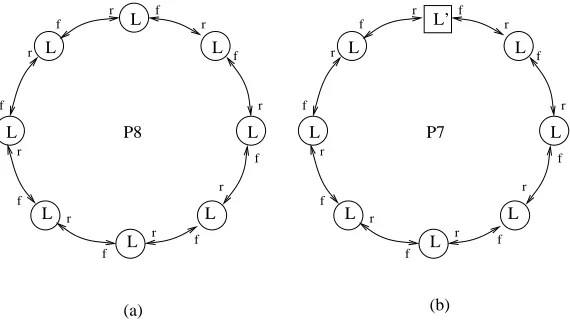
L L L’ L L f r r f r f f r r f r f r _f r f L L L L L L L L f r r f r f f r P8 r f r f r _f r f L L L P7 (a) (b)

Figure 2.2: (a) ring-structured LTS systemP8 and (b) ring-plus-structured LTS systemP7

Definition 2.2.2 A ring-plus-structured LTS system Pi is composed of LTSL0 and i > 1 instances of LTS Lsuch that each LTS synchronizes with its left and right neighbors with events f and r respectively. Formally,Pi is defined in CCS as

Pi = (L1 ||L2 ||... || Li) \ {h0, h1, ...hi }, where L0=L0[h0/f, h1/r],

L1=L[h1/f, h2/r],

...

Li=L[hi/f, h0/r].

(21)

2.3 General LTS systems and client/server LTS systems

Definition 2.3.1 A general LTS system Pi is composed of LTS Base and i instances of LTSL. Formally, Pi is defined in CCS as

Pi = (Base ||L1 ||L2 || ... || Li) \ I with

L1=L2= ... =Li=L, and I being the set of internal events. The setP ={ Pi |i >0} is referred to as a general LTS domain.

Definition 2.3.2 A client/server LTS system is defined as a set of LTSs satisfying the following properties:

1. One LTS, called the server LTS, synchronizes with other LTSs.

2. Other LTSs, called client LTSs, are instances of one or multiple LTS types1, synchro-nize with the server, and do not synchrosynchro-nize with each other.

3. Each client does not containτ transitions.

4. The server may contain τ transitions, but it does not have loops that contain τ transitions only.

5. No server or clients have deadlocks.

The set of client/server LTS systems with the same server and different numbers of clients is referred to as a client/server LTS domain.

2.4 Reachability graphs and model checking

Let P be a set of concurrent processes L1, L2, ..., and Lr, wherer > 1. Reachability analysis ofP involves deriving the reachability graph (RG) ofP, which contains all possible states of P, and analyzing the RG to detect deadlocks and other types of faults. The definition of a state of P depends on how processes are represented, how they interact with each other, and the level of accuracy. Assume that each process in P is represented by a sequential program, a state of P can be defined as [S1, S2, ..., Sr, other information], where Si,0 < i ≤ r, denotes the next statement to be executed by process Li and “other information” includes the values of all variables and the contents of all message queues. This

(22)

definition of a state provides complete information. However, since the size of RG(P) is an exponential function of the total number of processes, variables and message queues, this definition can be used in practice only ifPcontains a small number of simple processes. One alternative is to define a state of P as [S1, S2, ..., Sr]. This definition significantly reduces the size of RG(P), but the results of reachability analysis are inaccurate. Techniques for constructing RGsfor concurrent programs can be found in [PTY95] [Hol97].

RGs can be used for deadlock analysis as well as model checking, which was proposed by Queille and Sifakis [QS82], Clarke and Emerson [CE81] [CES86], and others [LP85]. Model checking verifies a behavioral property of a system through exhaustive enumeration (explicit or implicit) of all the states reachable by the system.

Formally, model checking is defined by E.M. Clarke [Cla99] as “Given a Kripke struc-ture M = (S, R, q0, AP, L) that represents a finite-state concurrent system and a

tem-poral logic formula f expressing some desired specifications, find out f(q0) = true or

f(q0) =f alse.”.

In this definition, Kripke structureM = (S, R, q0, AP, L) is an FSM whereS is a

non-empty set of states,R⊆S×S is the transition relation,q0∈S is the initial state,AP is a

finite set of atomic propositions, andL is the labeling function which assigns to each state of S the true/false value for the setAP of atomic propositions.

The temporal logic formula f, which can be either linear temporal logic or branching temporal logic, is based on the set AP of atomic propositions associated with the Kripke structureM. In this dissertation, we use CTL (Computation Tree Logic) [CE81] [Mc93] to express branching temporal logic defined as follows:

• Every atomic proposition g∈AP is a CTL formula.

• If f and g are CTL formulas, then so are ¬f, f ∨g, f∧g, AXf,EXf,A(fUg), and E(fUg)

CTL formulas are composed of path quantifiers and temporal operators. The path quantifiers include A (for all paths) and E (for some paths). The temporal operators include X (next time), U (until), F (eventually) and G (always). Temporal operators F and Gcan be viewed as being derived fromUaccording to the following rules:

(23)

• EGf = ¬A(trueU¬f)

Temporal logic can be used to express a broad range of specifications. For example, the liveness property of a concurrent program can be expressed as AG(AFg) where the atomic proposition g is defined as “one progress step is made”.

A reachability graph can be easily converted into a Kripke Structure with the labeling functionLbeing defined for each state. This is usually done in parallel with the generation of the reachability graph. For example, to perform model checking of the liveness property AG(AFg), the true/false value for the atomic proposition g (whether one progress step is made) can be assigned to each state during the construction of the reachability graph.

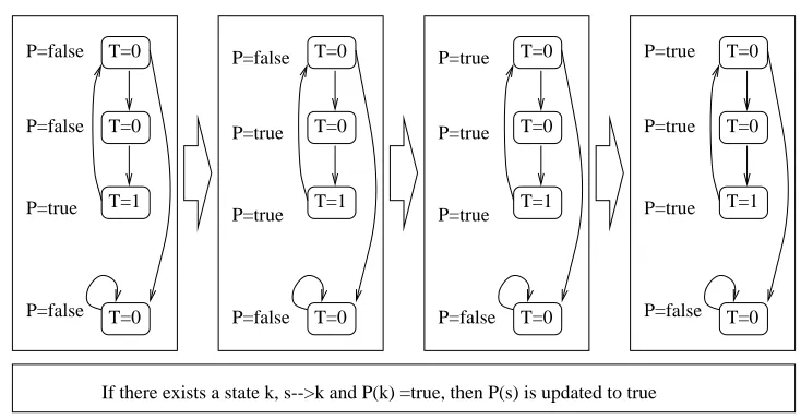
Fig. 2.3 and Fig. 2.4 show simple model checking algorithms for two CTL temporal logic formulas.

Initially, for all states with "T=1", P is set to be true, otherwise, P is set to be false. P="there exists an execution sequence such that ‘T=1’ eventually to be true"

If there exists a state k, s-->k and P(k) =true, then P(s) is updated to true

T=1 T=1 T=1 T=1

T=0 P=true P=false P=true P=true T=0 T=0 T=0 P=true P=false P=true P=true T=0 T=0 T=0 P=true P=false P=false P=true T=0 T=0 T=0 T=0 P=false P=false P=false P=true T=0

Figure 2.3: Recursive model checking algorithm for P: EF(“T=1”)

Definition 2.4.1 (Simulation)[Cla99] Given two Kripke structuresM = (S, R, q0, AP, L)

andM0 = (S0, R0, q0₀, AP, L0), a binary relationLR⊆S×S0is asimulationrelation between M andM0 if and only if for any two states s∈S ands0 ∈S0, ifLR(s, s0) then the following conditions hold

1. L(s) =L0(s0).

(24)

T=0 T=0 T=0 T=0

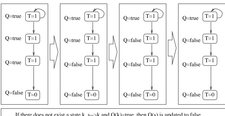
If there does not exist a state k, s-->k and Q(k)=true, then Q(s) is updated to false Initially, for all states with "T=1", Q is set to be true; otherwise, Q is set to be false

Q="there exists an execution sequence such that ‘T=1’ is always true"

T=1 T=1 T=1

Q=false

Q=false Q=true

Q=false Q=false

Q=false Q=true

Q=true

Figure 2.4: Recursive model checking algorithm forQ: EG(“T=1”)

3. For every states0₁such that R0(s0, s0₁), there iss1 such thatR(s, s1) andLR(s1, s01).

Structures M and M0 are said to be simulation equivalent (denoted as M ≡ M0) if there exists a simulation relationLRsuch that LR(q0, q00).

Theorem 2.4.1 [Mc93] [Cla99] Given two Kripke structuresMandM0, ifM ≡M0then for every CTL formulaf based on the atomic proposition set ofM (orM0),M |=f ⇔M0 |=f. In other words, M and M0 are exchangeable w.r.t. model checking.

2.5 Global and local deadlocks

2.5.1 Global and local deadlocks in a concurrent program

(25)

Let P be a concurrent program containing two or more processes. Assume that the number of states inRG(P) is finite. Informally,P is said to have a deadlock ifP can reach a state such that some process in P is blocked in this state and remains blocked forever. Lets be a state ofRG(P).

1. If a process in P is blocked in s and all states reachable froms, then this process is said to be deadlocked in sand sis said to be a deadlock state for this process. 2. s is said to be a deadlock state if at least one process of P is deadlocked in s. A

deadlock state s is said to be a global deadlock state if every process is s is either blocked or terminated; otherwisesis said to be a local deadlock state.

3. P is said to have a deadlock ifRG(P) contains at least one deadlock state. LetLbe a process ofP. If a statesofRG(P) is a deadlock state forL, then all states reachable from sare deadlock states forL.

Global and local deadlock can be defined as CTL formulas. For a concurrent program P, a global deadlock state is not a termination state and has no outgoing transitions. In order to define global deadlock as a CTL formula, we define an atomic proposition g for any state of RG(P) as “the current state is not a termination state and has no outgoing transitions”. The property of freedom from global deadlocks can be expressed as “AG(¬g)”. As for the property of freedom from local deadlocks, a set of atomic propositions need to be defined. Assume that a concurrent program P have m+ 1 processes L0, L1, ...Lm. Let atomic proposition gi,0≤i≤ m, for a state s of RG(P) be defined as “Li is blocked insand sis not a termination state”. Thus, the property of freedom from local deadlocks can be expressed as “¬(EF(AG(g0))∨EF(AG(g1))∨...∨EF(AG(gm)))”. In the formula, EF(AG(gi)) means the existence of a loal deadlock forLi.

Theorem 2.5.1 A concurrent program P has no global deadlocks if P has no local dead-locks for any process in P.

Proof Assume thatP has a global deadlock. Then each process ofPhas a local deadlock.

(26)

2.5.2 Global and local deadlocks in an LTS

A state sof an LTS L is said to be a global deadlock state ifs is reachable from the initial state of L and has no outgoing transitions. If such state s exists, LTS L is said to have a global deadlock. In this dissertation, we assume that the LTS for each process in a concurrent program has no global deadlock .

a b a c

L2 P1 P2

τ

τ c

L1 E1

F0

F1 E0

E1,F1 E1,F1

E0,F0 E0,F0

Figure 2.5: Illustration of deadlocks

Consider the following LTSs, which are shown in Fig. 2.5. L1 =a.b.L1

L2 =a.F1, F1 =c.F1

P1 = (L1||L2)\{a, b}

P2 = (L1||L2)\{a, b, c}

P1 has no global deadlock states, butP2 has a deadlock state (E1, F1).

Consider two LTSs P and P0. IfP ∼P0, then P has a global deadlock if and only if P0 has a global deadlock. However, P ≈P0 does not implies that P has a global deadlock if and only if P0 has a global deadlock. The reason is that process 0, which has only one state and no actions, is observationally equivalent to P3, which is defined as “P3 =τ.P3”.

Process0 has a global deadlock state, butP3 does not.

In the above example, state (E1, F1) of P1 has only one outgoing transition, which

is a c transition to (E1, F1). The c transition from (E1, F1) to (E1, F1) is a transition originally in L2. After entering (E1, F1), P1 will not execute transitions originally in L1.

So (E1, F1) is a local deadlock state inP1forL1. Below we formalize the concept of a local

(27)

Assume that LTS P is defined as (L1||L2||...||Ln)\I, where I is the set of internal events forP andLi,1≤i≤n, is the LTS of a process. For each transitiontinP, letpid(t) be defined as follows.

(a) Iftis a τ transition due to a synchronization betweenLi andLj, where 1≤i, j≤ n, pid(t) ={i, j} and t is said to involve transitions inLi andLj.

(b) If tis aτ transition originally inLi, 1≤i≤n, pid(t) ={i}.

(c) If t is a non-τ transition originally in Li, 1 ≤i≤ n, pid(t) ={i} and t is said to involve a transition inLi.

A state sinP is said to be a local deadlock state forLi,1≤i≤n, ifsand all states reachable from s do not have any outgoing transitions that include i in their pid sets. P is said to have a local deadlock for Li,1≤i≤n, ifP contains at least one local deadlock state forLi.

Based on the formal definition of local deadlocks, the following algorithm checks whether a state s of an LTS system P is a local deadlock state for process Li. If each state of P is not a local deadlock state for each process, thenP has no deadlocks.

1. Let queueOpenbe empty and let setV isited be empty. 2. Put statesinto queueOpen

3. If queueOpenis not empty, remove its first element g Otherwise, exit with state sbeing found to be a local deadlock state for processLi.

4. If there exists an outgoing transition t of g with i included in pid(t), exit with state sbeing found not to be a local deadlock state for process Li.

5. Put gintoV isited and append all states which are directly reachable fromg and are neither in Opennor inV isited at the end of queueOpen.

6. go back to step 3.

A global deadlock state inP is a local deadlock state for eachLi,1≤i≤n. Thus, we have the following theorem.

Theorem 2.5.2 Assume that LTSP is defined as (L1||L2||...||Ln)\I, whereI is the set of internal events forL. Each Li, 1≤i≤n, has no global deadlocks.

(28)

(b) Assume that Li and Lj, where 1 ≤i, j ≤n and i 6=j, are identical instances of the same LTS definition. P does not have local deadlocks for Li iff P does not have local deadlocks forLj.

(29)

Chapter 3

Review of Related Work

In Section 3.1, we briefly review previous work on alleviating the state explosion prob-lem in RA. In Section 3.2, we describe previous work on finding deadlock cutoff numbers.

3.1 Alleviating the state explosion problem

The efficiency of reachability analysis (RA) of a system depends on the size of the system’s reachability graph. The larger the reachability graph is, the more time and memory it takes to verify the system. The major obstacle of RA is the state explosion problem.

Considerable efforts have been spent on alleviating the state explosion problem. Many different techniques have been proposed, including partial-order reduction [GW91] [LC89] [Val91], symbolic model checking [Mc93], compositional techniques [YY91], abstraction [CGL94], and dataflow analysis [DC94] [MR90] [MR91].

Symbolic model checking [Mc93] was first proposed by E. M. Clarke and K. L. McMil-lan. It is able to verify complex systems by representing a large set of states in a compact

(30)

Partial-order reduction techniques have aroused significant interests in recent years. They take advantage of independent transitions in an interleaving model of a system. For a global stategof a concurrent system, partial-order reduction methods construct a subset T of the set of enabled transitions in g such that each transition in T remains enabled at every global state that can be reached from g by an execution of transitions not in T. After getting the subsetT (which is called apersistent set), partial-order reduction methods explore only the transitions inT. In contrast, the conventional reachability analysis explores each enabled transition in g. Thus, partial-order reduction methods only explore parts of the global state space that are sufficient for verifying certain properties. [Pel94] [GP93] [GW91].

Compositional techniques [KT96] [GS90] are divide-and-conquer approaches usually making use of abstraction capabilities of process algebra. Compositional techniques derive the reachability graph of sub-systems independently, simplify them after certain verifica-tions, and then hierarchically combine them to form the reachability graphs of larger parts of a complete system.

3.2 Finding deadlock cutoff numbers

AssumeP is a message-passing program with identical processes and contains exactly one process type T. To perform reachability analysis of P, the number of instances of T needs to be determined. If the number is large, reachability analysis of P needs huge memory and very long CPU time. If the number is small, we have little confidence on the correctness of P with larger numbers of instances of process type T inP. Although many techniques can be used to relieve the state explosion problem, one interesting question is that for the program P, can we find a number U such that under certain condition if P with U instances of T has no deadlocks, then P with more than U instances of T has no deadlocks? Such a number is called a deadlock cutoff number.

(31)

analyze programs with different topologies: star topology: symbolic reachability analysis broadcast topology: matrix equations ring topology: simple induction other topologies: induction with filters

For a ring-structured system with identical processes, he proposed an induction tech-nique and said that “the principle of induction states that if an observer cannot distinguish between two systems with i andi+ 1 processes even with an infinite input to both systems, then he also cannot distinguish system withiprocesses and any other system with more than

i processes ”. In the future work section of [Gar88], Garg said that “for application of the induction technique, we need to find a k such that the system withk processes is equivalent to a system with k+ 1 processes. It was easy in our examples wherek had small values (1

and 2). There needs to be a more general algorithm for selecting k ”.

(32)

Chapter 4

Using Observational Equivalence

for Deadlock Analysis of LTS

Systems

Equivalence checking is an important concept in process algebra. It is often used in compositional techniques to alleviate the state explosion problem. In this chapter, we present techniques using observational equivalence to find deadlock cutoff numbers. Sections 1 presents basic principles. Section 2, 3, and 4 show techniques for finding deadlock cutoff numbers for ring-structured LTS systems, ring-plus-structured LTS systems, and general LTS systems respectively. Section 5 presents empirical studies. Section 6 presents a brief comparison.

4.1 The environment of an LTS in an LTS system

For a systemP of LTSs L0, L1, L2, ..., Lm, it can be formally specified in CCS as P = (L0||L1||...||Lm)\I, where I is the set of internal events.

For each LTSLi, 0≤i≤m, inP, its environment is the composition of all other LTSs inP.

(33)

Envi = (L0||L1||...||Li−1||Li+1||...||Lm). 2

With the above definition,P can be rewritten as P = (Envi||Li)\I.

The following theorem provides a foundation for deadlock analysis using observational equivalence.

Theorem 4.1.1 LetL, Env1 and Env2 be LTSs. Let

System1 = (L||Env1)\I and

System2 = (L||Env2)\I.

Assume that Env1 ≈ Env2. System1 has no local deadlocks for L if and only if

System2 has no local deadlocks forL.

Proof Below we prove the “only if” part. The proof for the “if” part is omitted. Assume that System1 has a local deadlock forLs. There exists a local deadlock state

(qL₁, qEnv1

1 ) in LTSSystem1, whereqL1 andqEnv1 1 are states of LTSLandEnv1 respectively,

such that

(1)qL₀ −→t0 q₁L , whereq₀L is the initial state ofL, (2)qEnv1

0

t1

−→qEnv1

1 , whereq

Env1

0 is the initial state of Env1,

(3) (q₀L, qEnv1

0 )

t

−→ (q₁L, qEnv1

1 ), where (q0L, q

Env1

0 ) is the initial state of System1 and t

is an interleaving of t0 and t1, and

(4) (q₁L, qEnv1

1 ) and all states reachable from (q1L, qEnv1 1) do not have any outgoing

transitions involving transitions inL.

Because Env1 ≈ Env2, there exists a sequence t2 such that qEnv0 2

t2

−→ qEnv2

1 and

qEnv1

1 ≈qEnv1 2, where q0Env2 is the initial state of Env2 and t2 has the same non-τ action

sequence as t1. It follows that there exists a sequence t0 of an interleaving of t0 and t2,

such that (q₀L, qEnv2

0 )

t0

−→(qL₁, qEnv2

1 ), where (qL0, q

Env2

0 ) is the initial state ofSystem2, and

(qL

1, q

Env2

1 ) and all states reachable from (qL1, q

Env2

1 ) do not have any outgoing transitions

involving transitions in L. Therefore, (q₁L, qEnv2

1 ) is a local deadlock state in System2 for

L.

(34)

4.2 Deadlock analysis of ring-structured LTS systems

In Section 2.2, we defined ring-structured LTS systems and domains. Assume that a ring-structured LTS domain P contains multiple instances of an LTS L. Each process synchronizes with its left and right neighbors with eventsf andr respectively. For the sake of simplicity, it is assumed that each process communicates with its left and right neighbors with only one event. The discussion in this section can be easily extended to the situations where each instance communicates with its left and right neighbors with two or more events.

Theorem 4.2.1 LetP ={Pm|m >1} be a ring-structured LTS domain, wherePm is the ring-structured LTS system with m instances of L. Let Envm be the environment of the instance ofL inPm.

Env2 =L,

P2= (L[h0/f, h1/r]|| Env2[h1/f, h0/r])\{h0, h1},

fori >2,

Envi = (L[f /f, h/r]|| Envi−1[h/f, r/r])\{h},

Pi= (L[h0/f, h1/r]|| Envi[h1/f, h0/r])\{h0, h1}.

L L

L

L _P6

f r

f

r

f r

f

r f

f

r

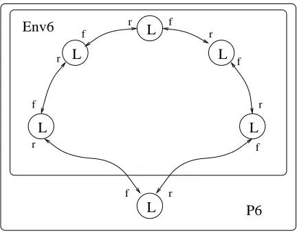
Env6

Figure 4.1: Ring-structured LTS systemP6

Assume thatLhas no global deadlocks and there exists an integerksuch thatEnvk≈ Envk+1. For any integer n > k,

(35)

(b)Pnhas no local deadlocks for L if and only if Pk has no local deadlocks for L. (c)Pn has no global deadlocks ifPk has no local deadlocks forL.

Proof Below we show the proof for (a). (b) is derived from (a) according to Theorem 4.1.1. (c) is derived from (b) according to Theorem 2.5.2.

Envk ≈Envk+1

= (L[f /f, h/r ]||Envk[h/f, r/r ])\{h} ≈(L[f /f, h/r ]||Envk+1[h/f, r/r ])\{h}

=Envk+2

We have Envk ≈ Envk+2. By using the same approach, we can show that Envk ≈ Envn for any n > k+ 2.

2

According to Theorem 4.2.1, for a ring-structured LTS domain P containing multiple instances of an LTSLthat has no global deadlock, if there exists an integerksuch thatPk has no local deadlocks for L and Envk ≈Envk+1, thenk is a deadlock cutoff number for

P. Below we show an algorithm to find a deadlock cutoff number for P. Algorithm Find DCN 4.2

Input L

{ if (Lhas a global deadlock)

{ DeadlockCutoffNumber Is Found =f alse; exit ;} k= 2;

while (true) {

if (Pk has a local deadlock forL)

{ DeadlockCutoffNumber Is Found= f alse; exit;} if (Envk≈Envk+1 )

{ DeadlockCutoffNumber Is Found= true; exit; } k=k+ 1;}

}

(36)

the above algorithm is that the loop in the algorithm might not terminate. To prevent this problem, we need to set an upper bound on the number of iterations of the loop.

4.3 Deadlock analysis of ring-plus-structured LTS systems

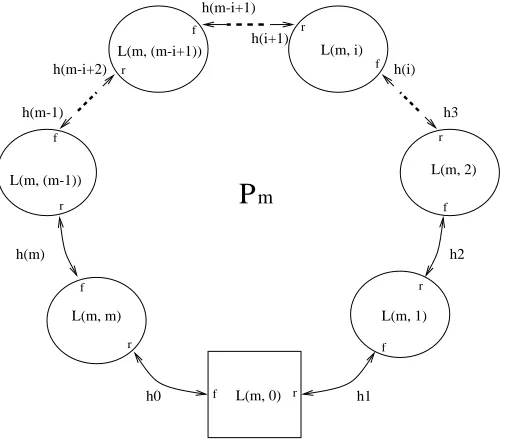
In Section 2.2, we defined ring-plus-structured LTS systems and domains. Assume that a ring-plus-structured LTS domain P contains processes with one of them being an instance of an LTSL0 and others being instances of an LTSL. Each process synchronizes with its left and right neighbors with eventsf andr respectively. For the sake of simplicity, it is assumed that each process communicates with its left and right neighbors with only one event. The discussion in this section can be easily extended to allow each process to communicate with its left and right neighbors with two or more events.

P

m

h0 h1

h(m-1)

h(i) h3

h2 h(m)

f

L(m, (m-1))

h(i+1) h(m-i+1)

r r

r

r r

r

f f

f

L(m, (m-i+1))

L(m, 0) L(m, m)

L(m, i)

L(m, 2)

L(m, 1) h(m-i+2)

Figure 4.2: Ring-plus-structured LTS systemPm

Theorem 4.3.1 LetP ={Pm|0≤m}be a ring-plus-structured LTS domain where Pm is the ring-plus-structured LTS system with minstances of L and one instance ofL0.

Pm = (L(m,0) || L(m,1) || ... || L(m,m)) \ {h0, h1, ...hm }, where L₍_m,₀₎=L0[h0/f, h1/r],

(37)

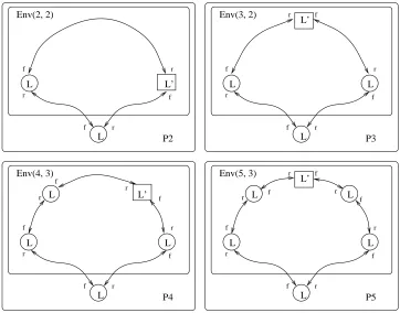
L L’ P2 f r f r r f L L L’ L P3 f r f r r f r f L L L L P4 f r f r r f f r L f L’ L L L’ L L P5 f r f r r f f r f r L

Env(4, 3) Env(5, 3)

r _f _r

Env(2, 2) Env(3, 2)

Figure 4.3: Env(m,i) in ring-plus-structured LTS systems

...,

L(m,i)=L[hi/f, h(i+1)/r],

...,

L₍_m,m₎=L[hm/f, h0/r].

LetEnv(m,i), 1≤i≤m, be the environment ofL(m,i) inPm. Env(m,i) = ( ( L(m,0) ||... L(m,i−1) || L(m,i+1) || ... || L(m,m))

\ { h0, ..., hi−1, hi+2, ...hm })[r/hi, f /hi+1]

Then Pm can be rewritten as

Pm = (Env(m,i) ||L[r/f, f /r] ) \ {r, f }, where 1≤i≤m−1.

Fig. 4.3 shows Env(2,2),Env(3,2),Env(4,2), andEnv(5,3) inP2,P3, P4 and P5

respec-tively.

(38)

(a)Env₍_k,i₎≈Env₍_n,i₎,

(b) Pn has no local deadlocks for L(n,i) if and only if Pk has no local deadlocks for L₍_k,i₎, and

(c)Pn has no global deadlocks ifPk has no local deadlocks forL(k,i).

Proof Below we show the proof for (a). (b) is derived from (a) according to Theorem 4.1.1. (c) is derived from (b) according to Theorem 2.5.2.

Env(k,i) ≈Env(k+1,i)

= (L[f /f, h/r ]|| Env₍_k,i₎[h/f, r/r ] ) \ {h } ≈( L[f /f, h/r ]|| Env₍_k₊₁_,i₎[h/f, r/r ] ) \ {h } =Env₍_k₊₂_,i₎

We have Env₍_k,i₎ ≈ Env₍_k₊₂_,i₎. By using the same approach, we can show that Env(k,i)≈Env(n,i) for any n > k+ 2.

2

According to Theorem 4.3.1, for a ring-plus-structured LTS domainP containing one LTS L0 and multiple instances of an LTSL, if there exist two integers k >0 and i, where 1≤i≤k, such thatPk has no local deadlocks forLi and Env(k,i) ≈Env(k+1,i), then k is

a deadlock cutoff number for P.

Below we show an algorithm to find a deadlock cutoff number forP. Algorithm Find DCN 4.3

Input L, L’

{ if (LorL0 has a global deadlock)

{ DeadlockCutoffNumber Is Found =f alse; exit ;} k= 1;

while (true) {

if (Pk has a local deadlock for anyL(k,i), 1≤i≤k)

{ DeadlockCutoffNumber Is Found= f alse; exit;}

if (there exists an integeri,1≤i≤k,such thatEnv₍_k,i₎≈Env₍_k₊₁_,i₎ ) { DeadlockCutoffNumber Is Found= true; exit; }

(39)

When the above algorithms terminates, ifDeadlockCutoffNumber Is Foundis true, then Pn, n > k, has no deadlocks and kis a deadlock cutoff number for P.

4.4 Deadlock analysis of general LTS systems

In Section 2.3.1, we defined general LTS systems and domains. LetP be a general LTS domain that contains a process type represented by an LTSL. LetBasebe the composition of LTSs in P that are not instances of L. (If P contains other process types, it is assumed that the number of instances of every other process type is fixed in P). Each instance of LTSL is an instance without relabeling operation.

Theorem 4.4.1 Let Let P={ Pm | 0 ≤ m } be a general LTS domain with Pm being the general LTS system containing LTS Base and m instances of L. Let Envm be the environment for an instance ofL inPm. Let I be the set of internal events inP. Thus,

Env2 =Base ||L,

P2= (L ||Env2)\I,

fori >2,

Envi =Envi−1 || L,

Pi= (L ||Envi)\I.

Assume thatL and Base have no global deadlocks and that there exists an integer k such thatEnvk≈Envk+1. For any integer n > k,

(a)Envk≈Envn,

(b)Pn has no local deadlocks for Lif and only ifPk has no local deadlocks for L, and (c)Pn has no global deadlocks ifPk has no local deadlocks forL.

Proof Below we show the proof for (a). (b) is derived from (a) according to Theorem 4.1.1. And (c) is derived from (b) according to Theorem 2.5.2.

Envk≈Envk+1= (Envk ||L)≈(Envk+1 || L) =Envk+2

We have Envk ≈ Envk+2. By using the same approach, we can show that Envk ≈ Envn for any n > k+ 2.

(40)

According to Theorem 4.4.1, we can have an algorithm similar to that in Section 4.2 to find a deadlock cutoff number for a general LTS domain.

To illustrate Theorem 4.4.1, consider a programQthat contains multiple instances of L, which is defined as

L=e.e.L+e.L

Let Qm be Q with m instances of L and let Envm be environment of an instance ofL in Qm+1. The set of internal events for Qis {e}. We have

Env2=L,

Q2= (L||Env2)\{e},

Env3=L||L,

Q3= (L||Env3)\{e},

Env4=L||L||Land

Q4= (L||Env4)\{e}.

We can show that Env2 6≈Env3

Env3 ≈Env4.

Since Q3 has no local deadlocks for L, Qn with n > 3 has no global deadlocks. So three is a deadlock cutoff number forL.

4.5 Empirical studies

(41)

e developed two solutions to the DP problem and verified these two solutions by using the toolcwb−nc[CPS93] and applying the theory in this chapter.

(a) Solution one

Initially, each philosopher holds his left fork and is thinking. When a philosopher feels hungry, he asks his right neighbor for his right fork. After eating, he returns the right fork to his right neighbor. When a philosopher is hungry and trying to get his right fork, his left neighbor can grab his left fork. When a hungry philosopher has no forks, he must wait for his left neighbor to return his left fork.

This solution is shown below as a ring-structure LTS domain in CCS, wherel, r, l, r, τ1,

and τ2 denote giving left fork, giving right fork, getting left fork, getting right fork, feeling

hungery, and eating respectively. Solution 1:

Think-with-left =l.Think-with-none + τ1.Hungry-with-left

Think-with-none = τ1.Hungry-with-none +l.Think-with-left

Think-with-both = r.Think-with-left

Hungry-with-left =l.Hungry-with-none + r.Hungry-with-both Hungry-with-none =l.Hungry-with-left

Hungry-with-both = τ2.Think-with-both

Philosopher = Think-with-left

Env2 = Philosopher

Env3 = ( Env2[f /r]|| Philosopher[f /l]) \ { f }

Env4 = ( Env3[f /r]|| Philosopher[f /l]) \ { f }

...

System2 = ( Env2[f0/l, f1/r] || Philosopher[f1/l, f0/r] )\ { f0, f1 }

...

We can show that

Env2 6≈Env3 andSystem2 is deadlock-free;

(42)

According to Theorem 4.2.1, three is a deadlock cutoff number for the above solution. Thus,Systemk is deadlock-free for any k >3.

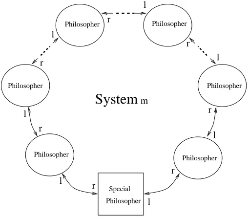
(b) Solution two

Initially, each philosopher holds his left fork and is thinking. When a philosopher feels hungry and is holding his left fork only, he asks his right neighbor for his right fork and his left neighbor can grab his left fork. When a philosopher is hungry and is holding his right fork only, his right neighbor can grab his right fork.

However, one special philosopher behaves in a different way. At beginning, this philoso-pher also holds his left fork and is thinking. When he is hungry and is holding his left fork only, his left neighbor can grab his left fork. When he is hungry and is holding his right fork only, he ask his left neighbor for his left fork and his right neighbor can grab his right fork.

This solution is shown below as a ring-plus-structured LTS domain in CCS, where l, r, l, r, τ1, and τ2 denote giving left fork, giving right fork, getting left fork, getting right

fork, feeling hungery, and eating respectively.

System

m

Philosopher Philosopher

Philosopher

l

l l l

l

l _r

r

r r r

r

Philosopher Special

Figure 4.4: Solution two for the DP problem

Solution 2:

(43)

Think-with-left =l.Think-with-none + τ1.Hungry-with-left

Think-with-both = r.Think-with-left + l.Think-with-right + τ1.Hungry-with-both

Think-with-right = r.Think-with-none + τ1.Hungry-with-right

Hungry-with-none = l.Hungry-with-left Hungry-with-both = τ2.Think-with-both

Hungry-with-left = r.Hungry-with-both

Hungry-with-right = l.Hungry-with-both+ r.Hungry-with-none

Think1-with-none = τ1.Hungry1-with-none

Think1-with-left = l.Think1-with-none + τ1.Hungry1-with-left

Think1-with-both = r.Think1-with-left + l.Think1-with-right + τ1.Hungry1-with-both

Think1-with-right = r.Think1-with-none + τ1.Hungry1-with-right

Hungry1-with-none = r.Hungry1-with-right Hungry1-with-both =τ2.Think1-with-both

Hungry1-with-left = r.Hungry1-with-both+ l.Hungry1-with-none Hungry1-with-right = l.Hungry1-with-both

Philosopher = Think-with-left

Special-Philosopher = Think1-with-left

Env₍₁_,₁₎ = Special-Philosopher

Env₍₂_,₁₎ = ( Philosopher[l/l, f /r] || Env₍₁_,₁₎[f /l, r/r]) \ { f } Env(2,2) = ( Env(1,1)[l/l, f /r] ||Philosopher[f /l, r/r] ) \ { f }

Env(3,1) = ( Philosopher[l/l, f /r] || Env(2,1)[f /l, r/r]) \ { f }

Env(3,2) = ( Philosopher[l/l, f /r] || Env(2,2)[f /l, r/r]) \ { f }

Env(3,3) = ( Env(2,2)[l/l, f /r] ||Philosopher[f /l, r/r] ) \ { f }

...

System1 = ( Env(1,1)[f0/l, f1/r]|| Philosopher[f1/l, f0/r] )\ { f0, f1 }

(44)

...

We can show that

Env(1,1) 6≈Env(2,1) and System1 is deadlock-free.

Env(2,1) ≈Env(3,1) and System2 is deadlock-free.

Env(2,2) 6≈Env(3,2) and System2 is deadlock-free.

According to Theorem 4.3.1, two is the deadlock cutoff number for the solution. So Systemk is deadlock-free for any k >2.

4.6 Comparisons

In Section 3.2, we reviewed two techniques for finding deadlock cutoff numbers for ring-structured systems. Here, we give a brief comparison between those two techniques and our approaches presented in this chapter.

As mentioned in section 3.2, Garg suggested that “we need to find a k such that the system with k processes is equivalent to a system with k+ 1 processes.”. But Gary does not formalize this concept and does not show how to find thisk. We have formally defined deadlock cutoff numbers and shown the use of observational equivalence to find deadlock cutoff numbers for ring-structured, ring-plus-structured, and general LTS systems.

(45)

Chapter 5

Using Projection Equivalence for

Deadlock Analysis of LTS Systems

In Chapter 4, we show algorithms for detecting deadlocks in LTS systems by using observational equivalence. More specifically, we show how to find an integer k, called a deadlock cutoff number, such that Envk and Envn are observationally equivalent for any n > k. We have applied these algorithms to several examples. Our results indicate that the use of observational equivalence fails to find deadlock cutoff numbers for some LTS systems that obviously have deadlock cutoff numbers. Consider the following client/server LTS domain defined as

P ={Pm|m >1}

Pm = (S||C1||C2||...||Cm)\{a, b} C1=C2 =...=Cm =C

S=a.b.S C=a.b.C

LetEnvm = (S||C1||C2||...||Cm−1),Pm can be rewritten as Pm = (Envm||C)\{a, b}.

(46)

a be k+ 1 andEnvk can not. Thus, the algorithm introduced in Section 4.4 fails to find a deadlock cutoff number for the example while one is obviously a deadlock cutoff number for the example.

Based on the above observation, we define a new equivalence relation called projection equivalence, which is weaker than observational equivalence. The use of projection equiva-lence increases the chance of finding a deadlock cutoff number for an LTS system if such a number exists.

In Section 5.1, we define projection operation and projection equivalence. In Section 5.2, we show the properties of projection equivalence. In Section 5.3 and Section 5.4, we present deadlock analysis of client/server LTS systems and ring-plus-structured LTS systems respectively by using projection equivalence. In Section 5.5, empirical studies are presented.

5.1 Projection equivalence

We first explain the concept of projection equivalence. Consider two LTS systems defined below.

System1 = (L||Env1)\I and

System2 = (L||Env2)\I

Assume that the behavior ofLinSystem1 is the same as that ofLinSystem2. From

the viewpoint of L, there is no difference betweenEnv1 andEnv2. In this situation, Env1

and Env2 are said to be projection equivalent with respect toL and I.

Let L and Env be LTSs and let LE be defined as LE= (L ||Env)\I,

where I is the set of internal event names for LE. We are interested in the behavior of L in LE. Such behavior is referred to as the projection of L in LE and is denoted as prj(L, Env, I). Transitions in LE can be divided into the following types:

1. τ transitions originally in L, 2. τ transitions originally in Env,

(47)

5. external transitions originally in Env.

To show the behavior ofL inLE, we modifyLE as follows:

1. For eachτ transition originally inL, replace it with a transition labeled (i, τ, j), where iand j denote the head and tail states respectively of theτ transition in L.

2. For each τ transition due to a synchronization between L and Env over event a, replace it with a transition labeled (i, a, j), where i and j denote the head and tail states respectively of the atransition inL that participated in the synchronization. 3. For each external transition originally inL, replace it with a transition labeled (i, ext, j),

wherei and j denote the head and tail states respectively of the transition in L and extis a new event name.

4. For each external transition originally inEnv, replace it with a τ-transition.

The modified LE is referred to as prj(L, Env, I). Fig. 5.1 shows an example of the projection operation.

2

a

1

τ

3 4

c

b _a

τ

b

c

Env

(1,a,2)

τ

(4,ext,1)

(3,b,4)

τ

(2, ,3)τ

L prj( L, Env, {a,b})

Figure 5.1: Illustration of projection operation

(48)

1. L

a

−→L0, a6∈I, a6∈I

prj(L,Env,I)(L,ext,L−→ 0)prj(L0,Env,I)

2. L

τ

−→L0

prj(L,Env,I)(L,τ,L−→0)prj(L0,Env,I)

3. L

a

−→L0, Env−→a Env0 prj(L,Env,I)(L,a,L−→0)prj(L0,Env0,I)

4. Env

τ

−→Env0

prj(L,Env,I)−→τ prj(L,Env0,I) 5. Env

a

−→Env0, a6∈I, a6∈I prj(L,Env,I)−→τ prj(L,Env0,I)

Definition 5.1.1 LetL, Env1 and Env2 be LTSs. Let I be a set of events. Assume that

prj(L, Env1, I) ≈prj(L, Env2, I). Lis said to have the same behavior in (Env1||L)\I and

(Env2||L)\I. Env1 and Env2 are said to beprojection equivalent with respect to L and

I, and this relation is denoted as Env1 ≈(L,I) Env2. 2

The fact that two LTSs areprojection equivalent with respect to a certain LTS does not imply that they are projection equivalent with respect to other LTSs. The follow-ing theorem shows that if two LTSs are observationally equivalent, they are projection equivalent with respect to any LTS.

Theorem 5.1.1 LetL,Env1andEnv2be LTSs. LetI be a set of events. IfEnv1≈Env2,

thenprj(L, Env1, I) ≈prj(L, Env2, I) and Env1 ≈(L,I)Env2.

Proof we define a binary relationS as

S={(prj(l, env1, I), prj(l, env2, I)) |env1 ≈env2, and

l, env1, and env2 are states of LTSsL, Env1, and Env2 respectively }.

Below we show thatS is an observation bisimulation. The proof consists of the following two parts:

(I) If (prj(l1, env1₁, I), prj(l1, env1₂, I)) ∈ S and prj(l1, env1₁, I) −→e prj(l2, env2₁, I), there must exist prj(l2, env2₂, I) such that (a) if e= τ,prj(l1, env1₂, I) −→τ∗ prj(l2, env₂2, I) and (prj(l2_{, env}2

1, I), prj(l2, env22, I))∈S; (b) ife6=τ,prj(l1, env12, I)

τ∗eτ∗

−→ prj(l2_{, env}2 2, I)

(49)

(II) If (prj(l1_{, env}1

1, I), prj(l1, env21, I))∈S and prj(l1, env21, I)

e

−→prj(l2_{, env}2

2, I), there

must exist prj(l2, env1₂, I) such that (a) if e= τ,prj(l1, env1₁, I) −→τ∗ prj(l2, env₁2, I) and (prj(l2, env₁2, I), prj(l2, env₂2, I))∈S; (b) ife6=τ,prj(l1, env1₁, I) τ−→∗eτ∗prj(l2, env2₁, I) and (prj(l2, env₁2, I), prj(l2, env₂2, I))∈S.

Below we show the proof for part (I). The proof for part (II) is similar and thus omitted. For part (I), assume that (prj(l1, env₁1, I), prj(l1, env₂1, I))∈S, which impliesenv1₁ ≈env1₂. There are five cases to consider.

Case 1:

l1 −→a l2, env1₁ −→a env₁2, a6=τ, ande= (l1, a, l2). In this case, becauseenv1

1 ≈env21, there must existenv22 such that

env₂1 τ−→∗aτ∗env₂2, env₁2 ≈env2₂. So prj(l1, env1₂, I)τ∗(l

1_,a,l2₎_τ∗

−→ prj(l2, env2₂, I)) and (prj(l2, env₁2, I), prj(l2, env₂2, I))∈S. Case 2:

l1 −→a l2, a6=τ, a6∈I, a6∈I, env₁1=env2₁, ande= (l1, ext, l2). In this case, prj(l1, env1₂, I)(l

1_,ext,l2₎

−→ prj(l2, env₂1, I)) and (prj(l2, env₁1, I), prj(l2, env₂1, I))∈S.

Case 3:

l1 −→τ l2, env1₁ =env2₁, and e= (l1, τ, l2). This case is similar to Case 2.

Case 4:

env₁1 −→a env₁2, a6=τ, a6∈I, a6∈I, l1=l2 and e=τ.

In this case, becauseenv₁1 ≈env₂1, there must existenv2₂ such that env₂1 τ−→∗aτ∗env₂2 and env2₁ ≈env₂2.

So prj(l1, env1₂, I)τ−→∗τ τ∗prj(l1, env₂2, I) and (prj(l1, env₁2, I), prj(l1, env₂2, I))∈S. Case 5:

env₁1 −→τ env₁2, l1 =l2, and e=τ.

In this case, becauseenv₁1 ≈env₂1, there must existenv2₂ such that env₂1 −→τ∗ env₂2 and env₁2≈env₂2.

(50)

So S is an observation bisimulation .

Thus,prj(L, Env1, I)≈prj(L, Env2, I)). In other words, Env1≈(L,I) Env2. 2

The following theorem, which is similar to Theorem 4.1.1, provides a foundation for deadlock analysis using projection equivalence.

Theorem 5.1.2 LetL, Env1 and Env2 be LTSs, and let I be a set of events. Let

System1 = (L||Env1)\I and System2 = (L||Env2)\I.

Assume that Env1 ≈(L,I) Env2. System1 has no local deadlocks for L if and only if

System2 has no local deadlocks forL.

Proof Below we show the proof for the “if” part. The proof for the “only if” part is similar and thus omitted.

If System1 has a local deadlock for L, there exists a state prj(L1, Env11, I) such that

prj(L, Env1, I)−→t prj(L1, Env11, I) wheretis a sequence of actions, and prj(L1, Env11, I)

and all states reachable fromprj(L1, Env₁1, I) do not have any outgoing transitions involv-ing transitions inL. Hence,prj(L1, Env1₁, I) and all states reachable fromprj(L1, Env₁1, I) have only τ-transitions as outgoing transitions. Since Env1 ≈(L,I) Env2 that means

that prj(L, Env1, I) ≈ prj(L, Env2, I), there exists a state prj(L2, Env22, I) such that

prj(L, Env2, I)

t0

−→ prj(L2_{, Env}2

2, I) where t0 and t have the same sequence of non-τ

events, prj(L1, Env₁1, I) ≈ prj(L2, Env₂2, I), and prj(L2, Env2₂, I) and all states reach-able from prj(L2, Env2₂, I) have only τ-transitions as their outgoing transitions. Thus, prj(L2, Env₂2, I) and all states reachable from prj(L2, Env2₂, I) do not have any outgoing transitions involving transitions in L. It follows that prj(L2, Env2₂, I) is a local deadlock state forL. Hence System2 has a local deadlock for L.

2

5.2 Properties of projection equivalence

(51)

to Theorem 4.1.1, can similar theorems be developed for projection equivalence. More specifically, we want to know whether the following conjecture is true.

“For an LTS domainP ={Pm|m >1} withPm containingm instances of an LTSL, letEnvm andEnv(m+1) be the environment of one instance ofLinPmandPm+1. Let

I be the set of internal events. ThusPm = (Envm||L)\I andPm+1 = (Envm+1||L)\I.

Assume that there exists an integerksuch thatEnvk≈(L,I)Env(k+1). For anyn > k,

Envk ≈(L,I) Envn.”

Unfortunately, the above conjecture is false. The following is a counter example for the conjecture.

P ={Pm|m >1},

Pm = (Base||L1||L2||...||Lm)\I with L1 =L2 =...=Lm=L,

Base=a.B1, B1 =a.B2+a.Base, B2 =a.a.B4+b.b.Base, B4=b.b.b.b.Base,

L=a.L0, L0 =b.L+c.L0, I ={a, b}.

Fig. 5.2 shows the graphical illustration of the example.

a

b

a

b

Base L

B1

B2

B4 B3

c

L’

Figure 5.2: An counter example

(52)

The above example shows that deadlock analysis using projection equivalence is not as straight-forward as that using observational equivalence. The example indicates that some condition between Pk and Pk+1 that is weaker than “Envk ≈Envk+1” but stronger than

“Envk ≈(L,I) Envk+1” needs to be satisfied in order to imply “Envk ≈(L,I) Envn for any n > k”. Such conditions will be presented in Sections 5.3 and 5.4 for client/server LTS domains and ring-plus-structured LTS domains respectively. In this section, we present two theorems on projection quivalence. These two theorems will be used in Sections 5.3 and 5.4.

Theorem 5.2.1 Let L1, L2, Env1, and Env2 be LTSs, and let I be the set of internal

events. Let

System1 = (L1||L2||Env1)\I and

System2 = (L1||L2||Env2)\I.

IfEnv1 ≈(L1||L2,I)Env2, then (Env1||L2)≈(L1,I)(Env2||L2).

Proof We define a binary relationS as

S={(prj(l1, env1||l2, I), prj(l1, env2||l2, I))| prj(l1||l2, env1, I)≈prj(l1||l2, env2, I), and

l1, l2, env1, and env2 are states of LTSsL1, L2, Env1,and Env2 respectively}.

Below we show that S is an observation bisimulation. Suppose that (prj(l₁1, env₁1||l1₂, I), prj(l₁1, env₂1||l1₂, I))∈S, which implies that prj(l1₁||l1₂, env₁1, I)≈prj(l1₁||l₂1, env₂1, I). Ifprj(l1

1, env11||l12, I)

f

−→prj(l2

1, env12||l22, I)), there are six cases, as shown below.

Case 1:

l1₁ −→a l2₁, l₂1=l₂2, env₁1 −→a env2₁, a6=τ, and f = (l1₁, a, l₁2).

In this case, prj(l1₁||l1₂, env₁1, I)−→e prj(l₁2||l1₂, env2₁, I), wheree= (l₁1||l1₂, a, l₁2||l1₂). Because prj(l1₁||l1₂, env1₁, I)≈prj(l1₁||l1₂, env₂1, I),

there must existprj(l2₁||l₂1, env₂2, I) such that

prj(l1₁||l₂1, env₂1, I)−→e prj(l2₁||l1₂, env₂2, I), wheree=τ∗(l1₁||l₂1, a, l2₁||l₂1)τ∗. So prj(l1₁, env1₂||l₂1, I)−→e prj(l₁2, env₂2||l1₂, I), wheree=τ∗(l1₁, a, l2₁)τ∗, and prj(l2₁||l1₂, env₁2, I)≈prj(l2₁||l₂1, env₂2, I).

Case 2:

Deadlock Analysis of Message-Passing Programs with Identical Processes

Identical Processes

To my wife

Yanyu Liu,

BIOGRAPHY

ACKNOWLEDGEMENTS

Contents

List of Figures

List of Tables

Chapter 1

Introduction

1.1

Problem statements

1.1.1

Reachability analysis and the state explosion problem

1.1.2

Message-passing programs with identical processes

1.1.3

Deadlock cutoff numbers

1.2

Summary of contributions

1.3

Organization of the dissertation

Chapter 2

Preliminary

2.1

LTS, CCS, and observational equivalence

2.1.1

Labeled transition systems (LTSs)

2.1.2

Process algebra CCS (calculus of communicating systems)

a

c

b

τ

τ

c

τ

τ

τ

τ

c

c

a

τ

b

c

τ

τ

2.1.3

Observational equivalence

2.2

Ring-structured LTS systems and ring-plus-structured

LTS systems

2.3

General LTS systems and client/server LTS systems

2.4

Reachability graphs and model checking

2.5

Global and local deadlocks

2.5.1

Global and local deadlocks in a concurrent program

2.5.2

Global and local deadlocks in an LTS

Chapter 3

Review of Related Work

3.1

Alleviating the state explosion problem

3.2

Finding deadlock cutoff numbers

Chapter 4

Using Observational Equivalence

for Deadlock Analysis of LTS

Systems

4.1

The environment of an LTS in an LTS system

4.2

Deadlock analysis of ring-structured LTS systems

4.3

Deadlock analysis of ring-plus-structured LTS systems