Sensorless MPPT Control Based On Left Invertibility

2036

Sensorless MPPT Control Based On Left

Invertibility

Imen Mrad, Jean Pierre Barbot, Lassaad Sbita

Abstract: This paper proposes a voltage sensorless Maximum Power Point Tracking (MPPT) controller for hybrid Photovoltaic (PV) system, which includes PV generator connected with DC DC SEPIC converter. This novel algorithm is based on Left Invertibility Problem (LIP) which consists of recovering the system’s inputs from its outputs and their derivatives. Thus, PV panel voltage was recovered based on hybrid high order sliding mode differentiator. Thanks to this method a simplified hardware configuration and a low cost system can be achieved. In addition, the partial observability problem of SEPIC converter was treated with respect to the Z (TN)-Observability concept and hybrid time trajectory. Simulation results are given using Matlab/ Simulink and then the proposed algorithm efficiency is verified.

Index Terms: Sensor less MPPT controller, SEPIC converter, Left Invertibility, finite time differentiator, Partial observability, Z(TN)-Observability, Hybrid time trajectory.

——————————  ——————————

1

I

NTRODUCTION BY dint of scarcity of traditional energy sources such as coal, oil or natural gas, renewable energy sources have been considered as sustainable alternative for future [1] [2]. Photovoltaic (PV) system is one of the most efficient power generation systems that convert the solar energy into various specific forms of electricity [3]. In this study a PV panel is chosen as energy source due to its benefits such as facility of implementation. Otherwise, PV power depends on ecological conditions such as radiance and temperature. According to the PV characteristics, there is a certain operating point at which the PV generator produces maximum power which is known as maximum power point (MPP). Therefore, to maximize the PV panel output power at different environmental conditions, maximum power point tracking (MPPT) is necessary in the PV system. In MPPT application, the main requirement is to use converter which have low input current ripple. The boost converter presents a high ripple in the load current, but a low current ripple on the PV side. And as compared with boost topologies, the Buck and its derived topologies have pulsating currents on the PV array side. Furthermore, with buck-boost topologies, a load voltage can be either lower or higher than the array voltage. But, the PV array and load current still have a pulsating. Besides, load voltage is inverted with buck-boost converter. Because of these above mentioned restraint, researchers are motivated to examine the possibility of employing single switch fourth order converter, namely single-ended primary inductance converter (SEPIC), Zeta [6] converter and Cuk [4] [5] converter to resolve those problems. These converters have four energy storage elements two inductances and two capacitors to transfer energy from input side to output side. In this work, a SEPIC is used to extract a maximum of power from PV generator because of its non pulsating input current, grounded switch and non-inverting output voltage.

Improvement of power electronics and semiconductor technology play an important role to reduce the cost of PV system and make the energy conversion of PV more efficient than ever before. In this research, a sensorless Maximum Power Point Tracking (MPPT) control is investigated. Thus, the PV voltage was reconstructed based on hybrid finite time differentiator [16]. Thanks to this method a simplified hardware configuration and a low cost system can be achieved with a single current input sensor. This proposed method is based on left invertibility problem LIP, it consists of determining the unknown inputs signals from the knowledge of the set of observations (i.e., the measurement outputs and it’s derivatives). During the last five decades, LIPs have been widely studied. They were being surveyed by Brockett and Mesarovic [7]. The algebraic criterion for invertibility and the construction of inverse system were given by Silverman [8]. In the case of non linear systems, it had begun with Hirschorn for single input single-output (SISO) [9]. And for Multi-input Multi-output (MIMO) [10], some geometric aspects and sufficient conditions for right invertibility problem were given in [11]. The proposed method can be resumed in the following figure.

2037 Based on left invertibility a sensorless Perturb and observe

(P&O) alogorithm was done, the PV voltage was reconstructed based on high order sliding mode differentiator coupled with an estimator, this estimated voltage value was after injected on the P&O MPPT algorithm which requires less hardware complexity and low-cost implementations.

The remaining of the paperis organized as follows: In Section 2, Modeling of global PV system was presented. Section 3 was devoted for MPPT based left invertibility where some recalls and definitions were given, after, left invertibility analysis for PV system is investigated and then, sensorless P&O algorithm.

2

P

HOTOVOLTAIC ENERGY CONVERSION

2.1 PV generator modeling

Pv cell can be substituted by an equivalent circuit as shown in Fig.2. It includes a power supply and a diode [18]. A current

p h

I occurs which depends on incident irradiation G, it crosses through the diode. And then, the diode absorbs light energy and transforming it directly into electric current [19]. The resulting Photovoltaic currentIp v is the difference between

p h

I andId which is reduced by the resistance Rs and Rp.

Fig.2 Equivalent Pv cell circuit

In accordance with the law of Kirchhoff one have :

p v

I =Ip h-Id-Ip (1) Knowing the following expression of the diode current:

e x p p v s p v 1

d s

s T

V R I

I I

N A V

    

 _{  } _

 

 

(2)

s

I : is the reverse saturation or leakage current of the diode. We can deduce the current supplied by the cell:





e x p p v s p v 1 p v s p v p v p h s

s T p

V R I

V R I

I I I

N A V R



    

  _   _

 

 

(3)

The thermal voltage V_T is defined by the following expression:

Let: c T

K T V

q

 and a N A Ks TC N A_s V_T

q

 

K : The Boltzmann constant =1.381 10-23 J/k. q: The charge of the electron =1.602.10-19 _C.

A: Ideality factor.

NS: The number of cells in series.

Tcel: The cell existing temperature.

With:

- Gr e f : irradiation at Standard Test Condition (STC) = (1000 W/m

2₎

- d T : T_{c e l}-T_{c e l r e f,} (Kelvin)

- Tc e l r e f, : Cell temperature at STC = 25+273 = 298K

- c s: Coefficient temperature of short circuit current (A/K). - : Photo current (A) at STC.

With:

- EG: Band gap energy (ev).

2.2 PV generator characteristics

According to the characteristics in the Fig.3, there is usually a single point on the curve I(V) or P(V), which is called: The maximum power point MPP, at this point the Photovoltaic system operates with maximum efficiency and produces maximum output power.

Fig.3 PV characteristics

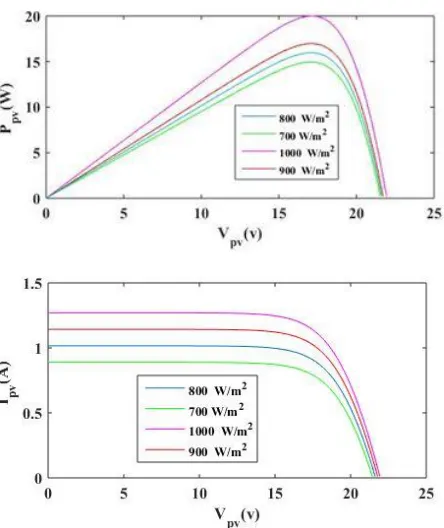
2.3Irradiation influence on the PV characteristics

The current and power of a PV module vary with the irradiation G, this is well shown in Fig.4, taking different



, .



( 4 ) p h p h r e f c s

r e f

G

I I d T

G



 

, p h r e f I

3

,

, ,

1 1

e x p ( 5 )

C G

s s r e f

C r e f A K C C r ef

T q E

I I

T T T

 

   

 _ _  _  _

 

2038 irradiation values (1000 to 700 W/m2_{) with constant}

temperature value T = 25 °C. Power/ Current increase with the sunshine. Besides, the augmentation in luminous flux increased the short-circuit current (Isc) as well as the

open-circuit voltage (Voc).

Fig. 4. Irradiation influence on the Ppv and Vpv

2.4 Temperature influence on the PV characteristic:

By varying the temperature values (T = 0 °C to T = 75 °C) and with a constant irradiation (1000 W/m2_{) as shown in Fig.5, one}

can note that the temperature has also a significant influence on the I(V)/P(V) characteristics of the PV generator. Thus, the increase in temperature causes the reduction in the open circuit voltage (Voc), as well as a decrease in the maximum power.

Fig. 5 Temperature influence on the Ppv and Vpv

2.5 DC/DC SEPIC converter modeling:

SEPIC can provide voltages which are greater than or equal to or less than the input voltage. Besides, it has a minimal actives components a simple controller, and clamped switching waves forms that provide a low-noise operation. The SEPIC has a fourth order model with four storage elements: two capacitors and two inductances as show in Fig.6. It is analogous to cuk and zeta topology. This converter is controlled through the switching element q.

Fig. 6 SEPIC circuit for (q=0)

1

2

1 1 2 4

1 1 1 1

2 1

1

3 3 4

2 2

4 1 3 4

2 2 2

0

1 1 1

1

1 f

1 1 1

L

i n

q

L R

x x x x V

L L L L

x x

C

R

x x x

L L

x x x x

C C R C



    



     

 

     

  





2039 1 2 1 1 1 1 2 3 1

3 2 3

2 2 4 1 4 2 1 1 1 1 n L q L i R

x x V

L L x x C R x x f x L L x x R C                       

SEPIC model can be represented by a hybrid matrix state equation, namely:

( ) _in

x A q x B V

y C x

      (6) Where: 1 2

1 1 1

1 1

2 2 2

2 2 2

1 1 0 1 0 0 ( ) 1 0

1 1 1

0 L

L

R q q

L L L

q q

C C

A q

R

q q

L L L

q q

C C C R

                  _{  }       _{  }        , 1 1 0 0 0 L B                  , C 0 0 0 1             

3

Left invertibility recalls:

Left invertibility problems have been studied in wide range of research and applications. It consists of recovering the unknown inputs signals and the states of a system from the knowledge of the set of observations (i.e., the measurement output and its derivatives). The diagram depicted in Fig.6 presents the principle of the left invertibility problem.

An effective solution for LIP is the ”differentiator” [20], because of its robustness and finite time convergence.

.

Fig. 6 Left invertibility problem

4

V

pv

reconstruction and observer design

4.1 Observability analysis

This section deal with observer designing for recovering PV panel volatgeV_{p v}. For given model it's easy to show that for (q=1) the SEPIC converter is not observable. Nevertheless, the system for (q=0) is completely observable.

Consider the observability matrix « Ґ » combining the information linked to the state and the input for q=0.

1 2 3 4

1 2 3 4

1 2 3 4

1 1 1 1

1 2 3 4

p v

p v

p v

p v

p v

y y y y y

x x x x V

y y y y y

x x x x V

y y y y y

x x x x V

y y y y y

x x x x V

y y y y y

x x x x V

                                                                     

1 2 2

2 1

1

1

0 0 0 1 0

1 1 1

0 0

1

C C C R

A B C D

C L

A

E F G H

L E

I J K L

2040 1

2

2 1 2

1 2

2 2

2 2

2

1 2 2 2 2

1

1 1 2

1

1

1

1 L

1 1 1

( )

L

L

L R A

R C L C

B

L C

R C

R C

D

L C L C R C

A R B D

E

L C C

A F

L 

  

  

    

 

  

 _{   }

 

 _{   }

 

 _{ }

 

2

2

2 2

1 2 2

1

1 1 2

1

2 2

1 2 2

L

L

L

C R _D

G

L C

A C D

H

L L R C

E R F H

I

L C C

E J

L

G R _H

K

L C

E G H

L

L L R C



  

 

 

  

  

   

  

 _{ }

 

 _{  }

 

 

  

 

The matrix Ґ is of full rank. Therefore, we are able to

reconstruct the states and the inputV_{p v}from the output x4 and

its derivatives for q=0. But for q=1, the system is unobservable. In this paper, left invertibility was investigated using Z(TN

)-observability concept *14+, *15+. This notion has the particularity of taking into account the partial observability of SEPIC converter by respecting the so-called hybrid time trajectory.

Definition 1 A hybrid time trajectory is a finite or infinite sequence of intervalsT_N  ( I ) N_{i i}N_0, such that:

- I_i  [ t_{i , 0}; t_{i ,1}[ fo r 0 i N ;

- For all i N :

,1 1 ,0

i i

m m

t t

 

-

0 ,0

t = t

in i

m m et ,1

t t

N e n d

m  m

Moreover, T_N is a ordered list of q associated to

0 1

T_N (q ,q , ...,q_N)with q_ithe value of qduring the time interval I_I

Definition 2 Consider the system (1), the variablez = Z t , x , V _in

is to said to be Z(TN)-observable with respect to hybrid time

trajectory TN for all trajectory (t, x, Vin) and (t, x', Vin') defined in

[tmini tmend], if the equality :







in



h t , x , V_in  h t , x ', V '

Implies



in





in



Z t , x , V  Z t , x ', V '

According to definition 1 and 2 the system (6) is observable in Z(TN) meaning. Indeed, it is Z(TN)-observable, if at least the

hybrid time trajectory contains one mode with q = 0. Consequently, the SEPIC is Z(TN)-observable under all PWM

(Piece Wise Modulation) control. Thus, a hybrid observer can be designed to estimate the vector X and to recover the voltage

V_{p v}.

4.2 Observer design

Based on Z (TN)-observablility, a hybrid observer can be

designed which combine the homogeneous finite differentiator *20+ for (q=0) (When the system is observable coupled with an estimator for all unobservable states for (q=1) by knowing their dynamic.

4.2.1 Recalls on finite time differentiator Consider a linear system on the following form:

With:

The finite time differentiator for this system is designed as:

𝑧 = 𝐴𝑧

𝑦 = 𝐶𝑧

(7)

𝐴 =

0

1

0

0

0

0

0

1

0

0

⋮

0

0

1

0

0

0

0

0

1

𝑃

₁

𝑃

₂

… 𝑃

_𝑛−1

𝑃

_𝑛

2041 Such that:

-- The gains Kiare chosen such that the following matrix is Hwirtz. Furthermore, those gains were selected sufficiently large such that the error dynamics (9) converge to zero in finite time, for more details see \cite,perruquetti2008finite}.

4.2.2 System transformation:

For observer designing SEPIC model (1) should be transformed in the form (7).

Consider the following transformation of SEPIC model for q=0:

Z  Tq0X  G VP V

Such that:

- (A B C D E F G H, , , , , , , ) which are already defined in the previous section.

-The finite time differentiator for SEPIC converter is defined as:

The observer design in the bases x:

As shown with this hybrid structure of observer (11), an estimator or a simple copy of the known dynamics works for q = 1 and a states reconstruction by using finite time observer works for q = 0.

And then :

1 1 q 0

ˆ ˆ ˆ

V_{P V}  G Z G T _ X

1 2 1 1 1

2 3 2 2 1

1 1 1 1

1 1 1 2 2

1 2 1 1

2 3

1

2 1

1 1 1

1 1 1 2

1 2 2 ˆ ˆ ( ) ˆ ˆ ( ) ( ) ( ) ( )

( 8 )

ˆ ˆ ( )

ˆ ( )

( )

n n n n

n n n n n

n n n n

n n n

z z k e

z z k e

z z k e

z k e P e P e P e

e e k e

e e k e

e e k e

e k e P e P e

                            _{    }            

( 9 )

n n P e         

And the observation error dynamic is:

( 1 )

( ) i i ( )

i e e s ig n e



   

1

1 1

1 n  _  _    1 2 1

1 0 0 0 0 1 0 0

0 0 0 1 0 0 0 0

n n k k K k k                   _    1 1 1 2 2 1 3 3 2 2 2 4 4

0 0 0 1

1 1 1

0

0 0

p v

C C C R

A B C D

E F G H

z x z x V g z x g z x      _{ }                     _  _                         1 2

1 1 1

1

, A

g g

L C L

 

1 2 1 1 1

2 3 2 2 1

3 4 3 3 1

4 4 4 1 1 1 2 2 3 3

1 4 4

ˆ ˆ ( )

ˆ ˆ ( ) ( 1 0 )

ˆ ˆ ( )

ˆ ( ) _{p v}

z z k e

z z k e

z z k e

z k e Pz P z P z P z E V

L              _{ }   _{     }   1 2 1

( 0 ) ( 0 )

3

1 2 3 4

4

1 1 1

2 2 1 1

( 0 )

3 3 1

4 4 1

ˆ _{0 1 0 0}

ˆ 0 0 1 0

ˆ ˆ

0 0 0 1

ˆ ˆ ( ) ( ) (1 ) ( ) ( (1 ) ) 1 q q q x x

X T T X

x

P P P P

2042

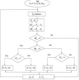
4.3 (P&O) based Left invertibility:

This section is dedicated for voltage sensorless MPPT controller. The algorithm (P&O) is chosen to improve the efficiency of the solar panel and extract the maximum of power. This algorithm requires less hardware complexity and low-cost. As shown in Fig.8, initially, Ppv is calculated by estimating the voltage Vp v based on finite time observer and

measuring the currentIp vof the solar array.

If dPpv=Ppv-P0reads positive, the system will keep perturbing

in the same direction by adding a small perturbation of the form ˆ

p v

V

 . Once it reads negative, the algorithm will bring the output power value back towards the maximum power point by adding a negative increment ˆ

p v

V

 . And the second value of Ppv is calculated by reconstructing the new value of ˆ

p v

V and

measuringIp v.

When the maximum power point is reached (dPpv=0), the

system operating point will start to oscillate constantly around this maximum point. The controller will track this operating

point and try to bring the Vˆp v of the solar array to perform at

this MPP.

5

Simulation and results:

The objectif of this section is to test and verify the performance of the sensorless P&O algorithm applied on PV system (SEPIC +PV generator), under the environment MATLAB-SIMILINKTM_{. The simulation model time step is 10}-6 _{s and}

SEPIC switching frequency is 20 kHz. Table 1 illustrates all parameters of the PV system. In order to verify the robustness of the proposed algorithm a change of irradiation was applied on the PV system as shown in Fig.8. Thus, the irradiation was changed from 1000 (W/m2_{) to 850 (W/m}2_{) at t = 0,2 s and from}

850 (W/m2_{) to 950 (W/m}2_{) at t = 0,6 s. One can note from Fig.9}

that PV panel power reaches its maximum from t =0,01s, this prove the validity of the voltage sensorless P&O algorithm and its capability to extract the maximum power even if without voltage sensor. Indeed, the sensorless P&O controller behavior converge toward the ordinary P&O behavior as shown in figures 8 and 9 . Besides, According to figures Fig.9 to Fig.12, it is noticeable that the proposed algorithm appear robustness against irradiation variation. Furthermore, it is clearly shown that based on observer (11) the vector

ˆ ˆ ₁ ˆ ₁ ˆ ₂

X  i L V c i L _converge toward of measured

statesX 



iL1 V c1 iL2



in finite time. Therefore, the estimation errors tend toward 0 from t=0.001s, as shown in figures Fig.13 to Fig.16. Consequently, according to those simulation results one can deduce the finite time convergence of the observer (11) and the capability of the left invertibility problem to reduce the number of sensor. Thus, by reconstructing the voltage Vpv with a sensorless P&O

controller one can extract the maximum of power from the PV panel.

Fig. 6 Flowchart of the sensorless P&O algorithm

TABLE1

PV SYSTEM PARAMETE RS

2043

Fig.8 Voltage Vpv (V)

Fig.10 Current iL1 (A)

Fig.11 Voltage VC1 (V)

Fig.12 Current iL1 (A)

Fig.13 Observation error

1

1 L

e  i  ̂

Fig.14 Observation error

1 1

2

ˆ

C C

e V V

Fig.15 Observation error

2 2

3 L ˆL

2044 Fig.16 Observation error

2 2

4

ˆ

C C

e V V

6

C

ONLUSION AND

F

UTURE WORK

:

In this research, a voltage sensorless MPPT method of the hybrid PV system is proposed. The available sensor of the output SEPIC converter is used to recover PV voltage and then we used this estimated value as input for P&O algorithm. A high order sliding mode differentiator coupled with an

estimator is suggested to recover Vpv. The simulation results presented in this work denote that the proposed method has considerable advantages. Furthermore, due to this method a simplified hardware configuration and a low cost system can be achieved. As a future work we would like to make an experimental study of this proposed MPPT algorithm on a real PV panel and SEPIC circuit.

References:

[1] N. Hidouri and L. Sbita, ―Water photovoltaic pumping system based on dtc spmsm drives,‖ Journal of Electric Engineering: Theory and Application, vol. 1, no. 2, pp. 111–119, 2010.

[2] M. Farhat, A. Flah, and L. Sbita, ―Photovoltaic maximum

power point

tracking based on ann control,‖ International Review on Modeling and Simulations, vol. 7, no. 3, pp. 474–480, 2014. [3] D. Nguyen and G. Fujita, ―Dynamic response evaluation of sensorless mppt method for hybrid pv-dfig wind turbine system,‖ Journal of International Council on Electrical Engineering, vol. 6, no. 1, pp.49–56, 2016. [4] P. Devika and R. Parackal, ―Sepic-cuk converter for pv

application

using maximum power point tracking method,‖ in 2018 International

Conference on Control, Power, Communication and Computing Technologies (ICCPCCT). IEEE, 2018, pp. 266– 272.

[5] M. Farhat and L. Sbita, ―Advanced fuzzy mppt control algorithm for

Photovoltaic systems,‖ Science Academy Transactions on Renewable

Energy Systems Engineering and Technology, vol. 1, no. 1, pp. 29–36,

2011.

[6] S. Arunraj, S. Murugesan, T. U. Nandhini, and K. Keerthana, ―A

novel zeta converter with pi controller for power factor

correction

in induction motor,‖ International Journal of Scientific Research in

Science and Technology, pp. 230–234, 2017.

[7] R. W. Brockett and M. Mesarovic, ―The reproducibility of multivariable systems,‖ Journal of mathematical analysis and applications, vol. 11, pp. 548–563, 1965. [8] L. Silverman, ―Inversion of multivariable linear systems,‖

IEEE transactions on Automatic Control, vol. 14, no. 3, pp. 270–276, 1969.

[9] R. M. Hirschorn, ―Invertibility of nonlinear control systems,‖ SIAM

Journal on Control and Optimization, vol. 17, no. 2, pp. 289–297, 1979.

[10]R. Hirschorn, “Invertibility of multivariable nonlinear control systems,”IEEE Transactions on Automatic Control, vol. 24, no. 6, pp.

855–865, 1979.

[11] W. Respondek, “Right and left invertibility of nonlinear control

systems,”in Nonlinear controllability and optimal control. Routledge, , pp. 133–176,2017.

[12]R. Goebel, J. Hespanha, A. R. Teel, C. Cai, and R. Sanfelice, ―Hybrid

systems: generalized solutions and robust stability,‖ in Proc. 6th IFAC symposium in nonlinear control systems. Citeseer, pp. 1–12, 2004.

[13] R. Goebel, R. G. Sanfelice, and A. R. Teel, ―Hybrid

dynamical

systems,‖ IEEE Control Systems, vol. 29, no. 2, pp. 28–93, 2009.

[14]W. Kang, J.-P. Barbot, and L. Xu, ―On the observability of nonlinear

and switched systems,‖ in Emergent problems in nonlinear systems

and control. Springer, pp. 199–216, 2009.

[15]W. Kang and J.-P. Barbot, ―Discussions on observability and invertibility,‖in NOLCOS, 2007.

[16]W. Perruquetti, T. Floquet, and E. Moulay, ―Finite-time observers: application to secure communication,‖IEEE Transactions on Automatic Control, vol. 53, no. 1, pp. 356– 360, 2008.

[17] A. Isidori, ―Nonlinear control systems,‖ Springer Science

& Business Media, 2013.

[18]MT. Chaichan and HA Kazem,”Experimental analysis of solar intensity on photovoltaic in hot and humid weather conditions,”International Journal of Scientific & Engineering Research, vol. 7, no. 3, pp. 91-960, 2016.

[19]MA Husain and A Tariq (2013). “Modeling of a standalone

Wind-PV Hybrid generation system using

MATLAB/SIMULINK and its performance

analysis”. International Journal of Scientific & Engineering Research, vol. 4, no. 11, pp. 1805-1811, 2013.

[20]A. Levant”Robust exact differentiation via sliding mode technique ”